Abstract
Due to small population size, Population Viability Analysis (PVA) of endangered species often pools all individuals into a single matrix to decrease variation in estimation of transition rates. These pooled populations may mask significant environmental variation among populations, affecting estimates. Using 10 years of population data (2000–2010) on the endangered plant Jacquemontia reclinata in Southeastern Florida, USA, I parameterized a stage-structured matrix model and calculated annual growth rates (lambdas)and elasticity for each year using stochastic matrix models. The metapopulation model incorporating actual dynamics of the two largest populations showed a lower occupancy rate and higher risk of extinction at an earlier time compared to a model that used the average of all natural populations. Analyses were consistent that incorporating population variation versus average dynamics in modeling J. reclinata demography results in more variation and greater extinction risk. Local variation may be due to both weather (including minimum winter temperature and total annual precipitation) and local disturbance dynamics in these urban preserves.
1. Introduction
Plants face a variety of threats that are putting many at risk of extinction [1,2]. Major threats include climate change [3], habitat loss and fragmentation [4], and dispersal limitations [5]. A major tool in assessing population dynamics and extinction risk is Population Viability Analysis (PVA), which typically uses stochastic matrix models to study individual populations and metapopulation dynamics [6,7,8,9,10,11]. Population viability analysis (PVA) is a widely used tool for assessing extinction risk and informing conservation decisions [12,13]. PVAs integrate demographic data into predictive models that evaluate the effects of different management scenarios on population persistence. Long-term studies are particularly needed but are rarely performed due to cost and short-term funding constraints [14].
In studying population dynamics of endangered plants, a major challenge is the trade-off between small population sizes and the ability to build accurate and robust population models [15,16]. When populations are small, pooling all observed demographic transitions into a single matrix may yield more stable estimates, but it comes at the cost of masking variation across populations. This is especially critical in fragmented urban landscapes, where populations are isolated and subjected to different environmental pressures. In fragmented landscapes, metapopulation theory provides an important framework for understanding the dynamics of spatially separated populations connected by occasional dispersal [11]. Metapopulation persistence depends on the balance between local extinctions and colonization, and it is especially relevant for urban preserves where habitat patches are isolated by roads and development. The concepts of source–sink dynamics [17] and landscape connectivity [18] are essential for assessing the viability of such species. In such contexts, metapopulation theory—which addresses population dynamics across a network of spatially separated but interacting populations—offers a more realistic framework [19,20,21,22].
The federally endangered Jacquemontia reclinata, endemic to coastal southeast Florida, is an ideal candidate for PVA given its restricted range, fragmented habitat, and long-term monitoring data. This study uses a 10-year demographic dataset (2000–2010) of the endangered Jacquemontia reclinata to (1) test whether pooling data across four populations biases long-term population growth estimates and (2) assess whether using average matrix values instead of actual population-specific matrices affects metapopulation projections across the species’ range. Environmental stochasticity, including year-to-year variation in precipitation and temperature, can have strong effects on population growth rates and extinction risk [23,24]. Incorporating such stochasticity into models increases the realism and relevance of PVA outputs. The collapse of one of the largest studied populations, the South Beach population in Palm Beach County between 2010 and 2020 [25], further underscores the urgency of adopting accurate models for conservation forecasting.
2. Materials and Methods
The study species, Jacquemontia reclinata (Convolvulaceae), is a perennial vine endemic (Figure 1) to coastal dunes in SE Florida, ranging historically from Martin to Miami-Dade Counties [26].
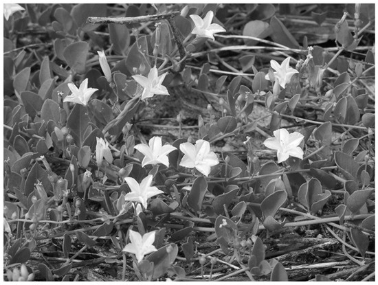
Figure 1.
Growth form and flowering morphology of Jacquemontia reclinata at South Beach (Palm Beach County, Florida). Plants exhibit a prostrate, twining growth habit with flowers borne terminally on elongating stems. Flowers are typically solitary, trumpet-shaped, and open during morning hours in the summer wet season. Photograph by author.
The plant grows as long runners from a central rooted axis and is not a climber (Figure 1). Flowering occurs during the rainy season at the tips of growing shoots and fruits are dry capsules that split open in the fall. Seeds are passively released and form a transient seed bank. The primary habitat is open dunes beyond the intertidal zone. Due to coastal development, habitat loss, and an increase in shrubby and woody vegetation on coastal dunes, the species was extirpated in multiple sites. It was listed as endangered in 1993. By 2011, less than 700 wild plants remained in a few protected populations [26].
Intensive study, propagation, and conservation efforts were led by Fairchild Tropical Botanical Garden in Coral Gables, Florida. In 2000, I initiated a long-term demographic study across four populations (two large and two small). A meter square grid was overlaid over all plants remaining at Crandon Park in Miami-Dade County, and South Beach (Figure 2), South Beach Inlet and Loggerhead Park in Palm Beach County.
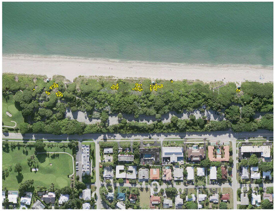
Figure 2.
Distribution of individual Jacquemontia reclinata plants at South Beach (Palm Beach County, Florida) in 2000. Each yellow circle indicates an individual plant mapped during baseline monitoring. South Beach was one of the two focal populations modeled in the population viability analysis and exhibited significant demographic variability and greater extinction probability during the study period. Aerial image source: Google Earth.
The corners of each m2 were marked using PCV pipes embedded into the sand. Within each grid, a sub grid of 16 25 by 25 cm using stringed meter squares was used to: (1) locate plant roots (which received a metal tag staked into the sand), (2) estimate occupancy (presence or absence in each subgrid), (3) estimate cover (Braun-Blanquet categories of 25%) and (4) record numbers of fruit. Based on previous studies, the number of seeds per fruit was estimated to be 3.47. This census was repeated annually until 2010.
A stage-size matrix model was constructed using five stages: (1) seeds in seed bank; (2) seedlings resulting from germinated seeds that are not yet reproductive, (3) reproductive stage of various sizes (small, medium, and large) based on area of ground covered (number of subgrids with a vegetative shoot) [26] (Figure 3).
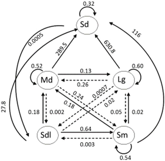
Figure 3.
Stage-structured life cycle diagram for Jacquemontia reclinata used in population viability modeling. Stages include seeds (Sd), seedlings (Sdl), and small (Sm), medium (Md), and large (Lg) reproductive plants. Solid arrows represent survival and transition probabilities; dashed arrows indicate shrinkage or regressive transitions. Shown is the average matrix of ten years (2000–2010).
Matrices resulting from the pooled data from all four populations (Average) were compared to matrix results from the two largest populations (Crandon and South Beach) analyzed individually [27]. Transition elements for all three matrices are in Appendix A. I used MATLAB code from Morris and Doak [12] to calculate growth rates (Lambda, λ) for each year. For each set of matrices, the individual growth rates per matrix per year were bootstrapped (300 iterations) to calculate 95% confidence intervals (CI) for the 10-year period. Elasticity of stage-transitions was calculated for the average matrix and the individual matrices over the 10-year period. The stochastic growth rate was calculated assuming an IID (independently and identically distributed) model and probability of quasi-extinction where N = 10 adult plants as the extinction threshold. The extinction threshold was set to 10 adult individuals per population, consistent with previous PVAs of clonal or rare plants. The quasi-extinction model ignores seeds in seed bank and seedlings as these are difficult for land managers to accurately census. The stochastic growth rate used a starting population of 29,308 seeds, 6 seedlings, 57 small adults, 73 medium adults, and 21 large adults.
I used RAMAS (Risk Analysis and Management Alternatives Software Version 5) Metapop [28] to simulate metapopulation dynamics across 10 populations. One model used the average matrix for all populations; the other used the actual transition matrices for Crandon and South Beach with the average matrix used for the remaining eight. The metapopulation was based on 10 natural populations remaining in 2000 (Crandon, High Taylor, Hillsboro Beach, South Inlet, South Beach, Red Reef, Atlantic Dunes, Lake Worth, Loggerhead, and Carlin Park, Appendix B). The model started with 763 adults among the 10 populations, assumed no catastrophes, the extinction threshold was 50 adults, density dependence was exponential on adult fertility and survival, seeds had dispersal, and there was no correlation among populations (Appendix B). Environmental stochasticity followed a lognormal distribution, a commonly used assumption in plant PVAs reflecting multiplicative demographic processes. Zero dispersal was assumed between populations, justified by the urbanized matrix and limited seed movement observed in field studies. Although some environmental synchrony may exist, there was no strong evidence for correlated dynamics, thus independence was assumed. The extinction threshold was set to 10 adult individuals per population, consistent with previous PVAs of clonal or rare plants. The model calculated average population size, metapopulation occupancy, local population occupancy, interval extinction risk, terminal extinction risk, and time to quasi-extinction.
To examine the relationship of λ to local weather, the weather data (minimum temperature, mean temperature, and annual precipitation) from the local airports in Palm Beach County and Miami-Dade county [29] were correlated with annual λ in the individual matrix models and with each other.
3. Results
3.1. Annual Population Dynamics and Growth Rates
Annual growth rates (λ) calculated from the average matrix ranged from 0.86 to 1.25, with a mean of 1.03 (±0.0415 SE; 95% Confidence Interval (CI): 0.989–1.071) (Table 1, Figure 4). Crandon’s annual λ ranged from 0.58 to 1.31, with a mean of 1.016 (±0.0702 SE; 95% CI: 0.870–1.162). South Beach ranged from 0.76 to 1.05, with a mean of 0.944 (±0.028 SE; 95% CI: 0.889–0.999). These values demonstrate greater interannual variability in individual populations compared to the pooled average model.

Table 1.
Annual growth rates (λ) for the average matrix and for Crandon and South Beach 1.
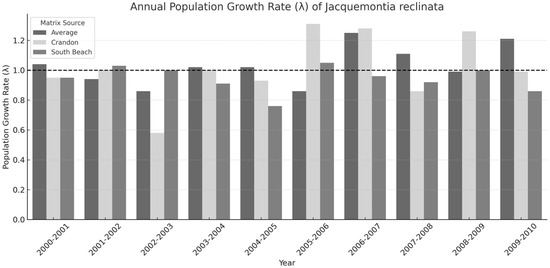
Figure 4.
Annual population growth rates (λ) of Jacquemontia reclinata from 2000 to 2010 based on three matrix models: the Average matrix (dim gray), Crandon population matrix (light gray), and South Beach matrix (medium gray). The horizontal dashed line at λ = 1.0 represents the threshold for stable population size. Bars reflect interannual variation in growth potential due to demographic stochasticity and site-specific differences.
3.2. Stochastic Growth Rates and Quasi-Extinction
The average matrix produced a stochastic growth rate of 1.018 (95% CI: 1.0155–1.0206). Crandon had a stochastic λ of 1.033 (95% CI: 1.0264–1.0395), while South Beach was 0.933 (95% CI: 0.9292–0.9365). Quasi-extinction risk (defined as <10 adults in 50 years) was <1% for the average matrix, 14% for Crandon, and 87% for South Beach (Figure 5 and Figure 6). These differences reflect the masking of risk in pooled estimates.
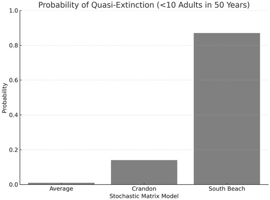
Figure 5.
Probability of quasi-extinction (<10 adult individuals) within 50 years for Jacquemontia reclinata under three matrix modeling approaches. Bars represent outcomes for the Average matrix, Crandon population matrix, and South Beach population matrix. The higher extinction probability for South Beach reflects elevated demographic variability and lower survivorship in that population.
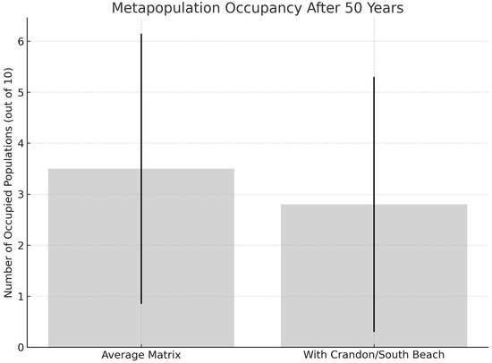
Figure 6.
Predicted metapopulation occupancy of Jacquemontia reclinata over 50 years under two modeling scenarios. The model using the Average matrix predicts greater population persistence than the model using actual matrices for Crandon and South Beach. Bars indicate mean number of occupied populations out of 10, with error bars representing 95% confidence intervals.
3.3. Elasticity Analysis
Elasticity analysis identified that the most influential transitions were adult survival (Lg→Lg and Md→Md) and transitions from seeds to seedlings (Table 2). In the average matrix, the largest elasticities were Lg→Lg = 0.38 and Md→Md = 0.27. In Crandon, these values were 0.42 and 0.23, respectively. South Beach showed lower elasticity in adult survival but higher values in seed transitions. These patterns suggest management should prioritize maintaining adult individuals and seedling recruitment.
Table 2.
Elasticity values of transition elements for the average matrix, Crandon and South Beach populations.
3.4. Metapopulation Dynamics
Using the RAMAS Metapop model parameters (Appendix B), the model was run (A) for the Average matrix elements for all populations and (B) using the actual matrices of Crandon/South Beach with the other populations using the Average matrix elements. Table 3 provides parameters of average population size at 50 yrs, metapopulation occupancy (Figure 6), local occupancy of Crandon and South Beach (Figure 7A), local extinction of Crandon and South Beach (Figure 7B), interval and terminal extinction risk (Figure 7C), and probability of quasi-extinction (Figure 7D). Using RAMAS, the average-matrix model predicted greater metapopulation persistence, with occupancy of 3.5/10 populations (95% CI: 0.9–6.2) and quasi-extinction in 41.9 years. The individual-matrix model showed lower occupancy (2.8/10, 95% CI: 0.3–5.3) and earlier quasi-extinction (34.2 years).
Table 3.
Model variables in RAMAS Metapop comparing 10 populations using the average matrix versus a model with actual dynamics of the two largest populations and average matrix transitions for the other 8 populations.
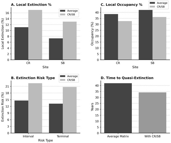
Figure 7.
(A–D) Comparative extinction metrics for Jacquemontia reclinata under two population viability modeling approaches: using the Average matrix for all populations versus using actual matrices for Crandon and South Beach (CR/SB), with the Average matrix applied to the remaining populations. (A) Comparison of local extinction probability (% of simulations where populations go extinct within 50 years) for Crandon and South Beach between the average matrix and the matrix with those actual populations. (B) Interval extinction risk (cumulative probability of extinction during the 50-year simulation) and terminal extinction risk (extinction probability at the end of the simulation periods between the average matrix and the matrix with those actual populations. (C) Local occupancy (% of simulations where populations persist after 50 years) between the average matrix and the matrix with those actual populations. (D) Predicted time to quasi-extinction (fewer than 10 adult individuals across the entire metapopulation) for the average matrix and the matrix with the actual populations. All bars reflect means from stochastic simulations in RAMAS Metapop, with consistent grayscale formatting used throughout for clarity.
Annual population growth varied much more in the Crandon and South Beach models compared to the Average matrix (Crandon had 5 years where λ > 1 and 5 years where λ < 1, South Beach had 2 years with λ > 1, 1 year where λ = 1, and 7 years where λ < 1. In contrast, the Average matrix had 6 years with λ > 1 and 4 years where (λ) < 1). All three estimates are significantly different based on the Confidence Interval. While Crandon had a higher stochastic growth rate than the Average matrix, it has a higher risk of extinction due to greater variation among years (the Average matrix shows less variation).
The two weather stations (Palm Beach Airport, Miami-Dade Airport) had significantly positive (p < 0.01) correlations in both mean temperature (r = 0.99) and precipitation (r = 0.68). I found a weak but consistent positive correlation between λ and annual precipitation (r = 0.32, p = 0.04), and a negative correlation with minimum winter temperatures (r = –0.36, p = 0.03).
4. Discussion and Conclusions
The results demonstrate that metapopulation models based on individual-year matrices produce substantially higher extinction risk estimates than models based on the averaged matrix, corroborating findings from earlier simulation studies [12]. The average matrix overestimates population growth and masks the influence of unfavorable years. This result emphasizes the importance of incorporating interannual variability when assessing viability for rare species subject to climatic extremes. The individual matrices for Crandon and South Beach exhibited more temporal variability, and the latter’s collapse from 2010 to 2020 highlights the danger of relying on average trends. This underscores the need for population-specific models in conservation planning.
The metapopulation model incorporating actual dynamics of CR and SB showed a lower occupancy rate and higher risk of extinction at an earlier time compared to a model that used the average of all natural populations (2000–2010, Average matrix). This is consistent with theoretical models of plant population dynamics where interpopulation variation within years is greater than temporal variation across populations. Thus, modeling of future dynamics of this species should use individual matrices calculated from each population, including both natural populations and new outplanting in both the natural range and outside the natural range in suitable habitats. Both MATLAB (r2024a) and RAMAS Metapopulation (Version 5) analyses were consistent that incorporating population variation versus average dynamics in modeling J. reclinata demography results in more variation and greater extinction risk.
The population at Crandon Park consistently exhibited the highest λ values and contributed most to metapopulation persistence, suggesting it functions as a demographic source [17]. In contrast, South Beach demonstrated consistently low λ and a high risk of local extinction, marking it as a potential sink. This aligns with metapopulation theory predictions [11] and is consistent with the observed local extinction of South Beach post-2010. South Beach’s high extinction risk was linked to lower adult survival elasticity and greater demographic variability, supporting its classification as a demographic sink. Conversely, Crandon exhibited characteristics of a source population, with higher adult survival rates and lower extinction risk. This source-sink framework offers a valuable lens for prioritizing management actions and targeting conservation investment. Source-sink dynamics may be compromised by the current habitat fragmentation into small populations embedded in an urban landscape that limits seed dispersal and plant density [25].
Elasticity analyses showed that large adult survival and medium-to-large adult transitions had the greatest influence on λ, mirroring findings in other rare plant studies [30,31,32,33]. Conservation actions should prioritize enhancing adult survival, promoting recruitment into large size classes, and managing threats that disproportionately affect reproductive adults [34,35]. Protecting adult plants from trampling and limiting dense dune vegetation through physical removal or controlled burns are some of the main management techniques used in managing populations of J. reclinata [25].
Local variation may be influenced by specific weather factors such as minimum winter temperatures and annual precipitation. The modest positive correlation between annual λ and both precipitation and minimum winter temperature, suggests that climate variability influences population growth, likely through effects on recruitment and survival. Incorporating environmental stochasticity using a lognormal distribution, as supported by Lande [23] and Menges [24], provided a more realistic extinction risk estimate under projected future climate variability [36]. Including such predictors in future models could improve forecasting accuracy and inform adaptive management under climate change as well as by local disturbance dynamics, including both natural events and human activities within these urban preserves.
This finding is important in the actual dynamics of the species from 2010 to 2020, where one of the largest natural populations (SB in this study) collapsed [25], declining from over 200 plants to just six remaining plants. This was not predicted from the metapopulation model that used the average of all natural populations but was shown as possible when using the actual dynamics from that subpopulation. The higher rate of extinction is warranted due to the highly fragmented populations that face both natural (hurricanes, storm surge, natural succession, climate change) [36] and anthropogenic impacts (trampling, arson fires, landscaping [37,38]. This approach, however, will entail higher costs as it will require more sampling across individual populations in this highly urbanized landscape. An approach that incorporated greater spatial sampling to account for the variation observed could be modified to be performed on a non-annual basis, thus mitigating some of the costs of annual monitoring. Based on observed stochasticity, I recommend a triannual (every 3 years) monitoring strategy that balances cost with ecological sensitivity. This can be complemented by citizen science, using volunteers trained in standardized protocols to monitor survival, flowering, and recruitment [25].
These findings underscore the value of using long-term demographic data and multiple matrix models in PVAs. They also highlight the urgency of management interventions that buffer small populations from stochastic threats and habitat degradation. This study provides critical insights for the conservation management of Jacquemontia reclinata, a federally endangered and endemic species. Future research should aim to refine estimates of the minimum viable population size, which will inform targeted mitigation strategies to restore natural populations and identify suitable outplanting sites for long-term survival. Although our findings indicate ongoing population declines in South Florida, the modeling techniques employed—along with increased public and scientific awareness—have contributed to reducing the species’ overall extinction risk [25]. Importantly, this work underscores the value of demographic modeling in guiding conservation decisions, not only for J. reclinata but also as a framework for managing other endangered plant species facing similar threats.
Funding
This research was funded by U.S. Fish and Wildlife Service Grant 401815G033 and 1448-40181-99-G-173, The Florida Fish and Wildlife Conservation Commission NG 02-012, Florida Department of Agriculture and Consumer Services #015982, #014880, and #013925, and the Florida Native Plant Society. Additional financial support for travel and lodging was provided by Valdosta State University, Georgia Southern University, and Fairchild Tropical Botanical Garden.
Data Availability Statement
The original contributions presented in this study are included in the article. Further inquiries can be directed to the corresponding author.
Acknowledgments
The author acknowledges Fairchild Tropical Botanical Garden, The Institute for Regional Conservation, and the U.S. Fish and Wildlife Service for support for organizing the 2024 “Beach Jacquemontia Virtual Summit” where these ideas were developed.
Conflicts of Interest
The authors declare no conflicts of interest. The funders had no role in the design of the study; in the collection, analyses, or interpretation of data; in the writing of the manuscript; or in the decision to publish the results.
Appendix A. Transition Matrix Elements for Average Matrix, Crandon, and South Beach
Appendix A.1. Average Matrix
| 2000–2001 | |||||
| sds | sdlgs | Small | med | large | |
| sds | 0.318 | 0 | 151.2211 | 169.6846 | 739.2752 |
| sdlgs | 0.000496 | 0 | 0 | 0 | 0 |
| small | 0 | 0.777778 | 0.77193 | 0.39726 | 0 |
| med | 0 | 0.088889 | 0.157895 | 0.465753 | 0.428571 |
| large | 0 | 0 | 0 | 0.082192 | 0.571429 |
| 2001–2002 | |||||
| sds | sdlgs | Small | med | large | |
| sds | 0.318 | 52.62833 | 123.3167 | 174.3177 | 537.0789 |
| sdlgs | 3.91 × 10⁻⁵ | 0 | 0 | 0 | 0 |
| small | 0 | 0.666667 | 0.642857 | 0.160714 | 0.166667 |
| med | 0 | 0.166667 | 0.214286 | 0.589286 | 0.111111 |
| large | 0 | 0 | 0.014286 | 0.160714 | 0.722222 |
| 2002–2003 | |||||
| sds | sdlgs | small | med | large | |
| sds | 0.318 | 17.35 | 54.78049 | 114.6801 | 400.4833 |
| sdlgs | 0.00054 | 0 | 0.003352 | 0.002757 | 0.001244 |
| small | 0 | 1 | 0.52459 | 0.313725 | 0 |
| med | 0 | 0 | 0.180328 | 0.54902 | 0.304348 |
| large | 0 | 0 | 0 | 0 | 0.521739 |
| 2003–2004 | |||||
| sds | sdlgs | small | med | large | |
| sds | 0.318 | 20.33333 | 145.1269 | 184.0627 | 493.8462 |
| sdlgs | 0.000704 | 0 | 0.0043 | 0.003023 | 0.000873 |
| small | 0 | 0.666667 | 0.557692 | 0.222222 | 0 |
| med | 0 | 0 | 0.192308 | 0.511111 | 0.083333 |
| large | 0 | 0 | 0.057692 | 0.088889 | 0.833333 |
| 2004–2005 | |||||
| sds | sdlgs | small | med | large | |
| sds | 0.318 | 149.22 | 110.5891 | 372.688 | 647.6471 |
| sdlgs | 0.000722 | 0 | 0.009608 | 0.006114 | 0.00297 |
| small | 0 | 0.777778 | 0.391304 | 0.257143 | 0 |
| med | 0 | 0.222222 | 0.282609 | 0.4 | 0.411765 |
| large | 0 | 0 | 0 | 0.142857 | 0.470588 |
| 2005–2006 | |||||
| sds | sdlgs | small | med | large | |
| sds | 0.318 | 38.26667 | 110.9391 | 244.5814 | 186.6429 |
| sdlgs | 9.53 × 10⁻⁵ | 0 | 0.005146 | 0.003495 | 0.001359 |
| small | 0 | 0.777778 | 0.514286 | 0.222222 | 0.214286 |
| med | 0 | 0.055556 | 0.257143 | 0.527778 | 0.357143 |
| large | 0 | 0 | 0 | 0.111111 | 0.285714 |
| 2006–2007 | |||||
| sds | sdlgs | small | med | large | |
| sds | 0.318 | 0 | 171.2941 | 401.8182 | 976.9412 |
| sdlgs | 0.000956 | 0 | 0 | 0 | 0 |
| small | 0 | 0.166667 | 0.512821 | 0.163636 | 0 |
| med | 0 | 0.5 | 0.307692 | 0.527273 | 0.111111 |
| large | 0 | 0.083333 | 0.051282 | 0.254545 | 0.777778 |
| 2007–2008 | |||||
| sds | sdlgs | small | med | large | |
| sds | 0.318 | 0 | 127.0847 | 527.2727 | 965.1304 |
| sdlgs | 0.000528 | 0 | 0 | 0 | 0 |
| small | 0 | 0.37037 | 0.4375 | 0.254545 | 0.043478 |
| med | 0 | 0.407407 | 0.28125 | 0.527273 | 0.304348 |
| large | 0 | 0.074074 | 0 | 0.127273 | 0.608696 |
| 2008–2009 | |||||
| sds | sdlgs | small | med | large | |
| sds | 0.318 | 0 | 93.7868 | 190.4848 | 418.9713 |
| sdlgs | 0.000275 | 0 | 0.003106 | 0.002112 | 0.000994 |
| small | 0 | 0.529 | 0.5 | 0.212121 | 0.054054 |
| med | 0 | 0.353 | 0.37931 | 0.560606 | 0.27027 |
| large | 0 | 0.059 | 0.034483 | 0.136364 | 0.594595 |
| 2009–2010 | |||||
| sds | sdlgs | small | med | large | |
| sds | 0.318 | 0 | 72.2291 | 515.1879 | 942.0025 |
| sdlgs | 0.000917 | 0 | 0 | 0 | 0 |
| small | 0 | 0.667 | 0.55102 | 0.231884 | 0.029412 |
| med | 0 | 0 | 0.265306 | 0.536232 | 0.205882 |
| large | 0 | 0 | 0.020408 | 0.202899 | 0.617647 |
Appendix A.2. Crandon
| 2000–2001 | |||||
| sds | sdlgs | small | med | large | |
| sds | 0.258405 | 0 | 72.05394 | 100.4463 | 260.0213 |
| sdlgs | 0 | 0 | 0 | 0 | 0 |
| small | 0 | 0.777778 | 0 | 0.133206 | 0 |
| med | 0 | 0.088889 | 0.781085 | 0.532825 | 0.374674 |
| large | 0 | 0 | 0 | 0.266412 | 0.624457 |
| 2001–2002 | |||||
| sds | sdlgs | small | med | large | |
| sds | 0.258405 | 0 | 1.292023 | 5.168094 | 16.92551 |
| sdlgs | 0.000412 | 0 | 0.00206 | 0.008242 | 0.026992 |
| small | 0 | 0.891241 | 1 | 0.166667 | 0.25 |
| med | 0 | 0 | 0 | 0.583333 | 0 |
| large | 0 | 0 | 0 | 0.25 | 0.75 |
| 2002–2003 | |||||
| sds | sdlgs | small | med | large | |
| sds | 0.258405 | 0 | 0.471558 | 2.697879 | 21.59961 |
| sdlgs | 0 | 0 | 0 | 0 | 0 |
| small | 0 | 0.891241 | 0 | 0.075931 | 0 |
| med | 0 | 0 | 0 | 0.303724 | 0.289526 |
| large | 0 | 0 | 0 | 0 | 0.579139 |
| 2003–2004 | |||||
| sds | sdlgs | small | med | large | |
| sds | 0.258405 | 0 | 0.343287 | 29.64709 | 169.211 |
| sdlgs | 0.00119 | 0 | 0.002008 | 0.16565 | 0.857746 |
| small | 0 | 0.685714 | 0.786843 | 0 | 0 |
| med | 0 | 0.171429 | 0 | 0.686573 | 0 |
| large | 0 | 0 | 0 | 0.137315 | 0.908127 |
| 2004–2005 | |||||
| sds | sdlgs | small | med | large | |
| sds | 0.258405 | 0 | 7.71371 | 21.9394 | 102.1896 |
| sdlgs | 0.000635 | 0 | 0.023807 | 0.06285 | 0.256766 |
| small | 0 | 0.333333 | 0 | 0.214402 | 0 |
| med | 0 | 0.666667 | 0 | 0.428804 | 0.325894 |
| large | 0 | 0 | 0 | 0.214402 | 0.651886 |
| 2005–2006 | |||||
| sds | sdlgs | small | med | large | |
| sds | 0.2584 | 0 | 4.539806 | 13.69448 | 202.1357 |
| sdlgs | 0.005464 | 0 | 0.117152 | 0.354515 | 5.33477 |
| small | 0 | 0.5 | 0.81943 | 0.272251 | 0.400609 |
| med | 0 | 0.214286 | 0 | 0.544584 | 0 |
| large | 0 | 0.142857 | 0 | 0 | 0.400609 |
| 2006–2007 | |||||
| sds | sdlgs | small | med | large | |
| sds | 0.258405 | 0 | 16.19738 | 77.42865 | 117.947 |
| sdlgs | 0.00138 | 0 | 0.118655 | 0.415112 | 0.630074 |
| small | 0 | 0.266667 | 0.145845 | 0.175837 | 0.0625 |
| med | 0 | 0.333333 | 0.437534 | 0.4689 | 0.499997 |
| large | 0 | 0.2 | 0.145845 | 0.351675 | 0.437498 |
| 2007–2008 | sds | sdlgs | small | med | large |
| 0.258405 | 0 | 11.78804 | 88.0838 | 217.5466 | |
| sds | 3.31 × 10⁻⁵ | 0 | 0.001957 | 0.01334 | 0.028822 |
| sdlgs | 0 | 0.4 | 0 | 0.168968 | 0.060357 |
| small | 0 | 0.342857 | 0.770705 | 0.591387 | 0.482857 |
| med | 0 | 0.085714 | 0 | 0.084484 | 0.4225 |
| large |
| 2008–2009 | |||||
| sds | sdlgs | small | med | large | |
| sds | 0.258405 | 0 | 12.81993 | 115.3711 | 156.2847 |
| sdlgs | 0.000704 | 0 | 0.038334 | 0.32958 | 0.430226 |
| small | 0 | 0.4375 | 0 | 0.212056 | 0 |
| med | 0 | 0.416667 | 0.455824 | 0.636167 | 0.123781 |
| large | 0 | 0.104167 | 0.455824 | 0.106028 | 0.866469 |
| 2009–2010 | |||||
| sds | sdlgs | small | med | large | |
| sds | 0.258405 | 0 | 6.750173 | 37.68633 | 88.33516 |
| sdlgs | 0 | 0 | 0 | 0 | 0 |
| small | 0 | 0.354167 | 0.221753 | 0.142119 | 0 |
| med | 0 | 0.354167 | 0.665259 | 0.710594 | 0.124999 |
| large | 0 | 0.229167 | 0 | 0.142119 | 0.874995 |
Appendix A.3. South Beach
| 2000–2001 | |||||
| sds | sdlgs | small | med | large | |
| sds | 0.258405 | 0 | 13.85222 | 45.10203 | 97.5719 |
| sdlgs | 9.84 × 10⁻⁵ | 0 | 0.005664 | 0.017904 | 0.037486 |
| small | 0 | 0.860417 | 0.736519 | 0.468612 | 0 |
| med | 0 | 0 | 0.194961 | 0.468612 | 0.991423 |
| large | 0 | 0 | 0 | 0.022315 | 0 |
| 2001–2002 | |||||
| sds | sdlgs | small | med | large | |
| sds | 0.258405 | 0 | 24.07305 | 98.09033 | 98.51992 |
| sdlgs | 0.000249 | 0 | 0.028333 | 0.103135 | 0.096318 |
| small | 0 | 0.666667 | 0.597037 | 0.126421 | 0 |
| med | 0 | 0.166667 | 0.204698 | 0.632106 | 0 |
| large | 0 | 0 | 0.017058 | 0.158026 | 0.985721 |
| 2002–2003 | |||||
| sds | sdlgs | small | med | large | |
| sds | 0.2584 | 0 | 18.45143 | 84.10765 | 165.546 |
| sdlgs | 0.000457 | 0 | 0.0378 | 0.153805 | 0.29301 |
| small | 0 | 1 | 0.676329 | 0.362513 | 0 |
| med | 0 | 0 | 0.186573 | 0.604188 | 0.428041 |
| large | 0 | 0 | 0 | 0 | 0.570722 |
| 2003–2004 | |||||
| sds | sdlgs | small | med | large | |
| sds | 0.258405 | 0 | 11.39434 | 13.59808 | 18.52254 |
| sdlgs | 0.000611 | 0 | 0.033646 | 0.037588 | 0.045735 |
| small | 0 | 0.6 | 0.541852 | 0.221838 | 0 |
| med | 0 | 0.2 | 0.18847 | 0.53875 | 0.239477 |
| large | 0 | 0 | 0.070676 | 0.095074 | 0.718432 |
| 2004–2005 | |||||
| sds | sdlgs | small | med | large | |
| sds | 0.258405 | 0 | 15.57881 | 71.32863 | 144.9046 |
| sdlgs | 0 | 0 | 0 | 0 | 0 |
| small | 0 | 0.666667 | 0.482639 | 0.256071 | 0 |
| med | 0 | 0.222222 | 0.271485 | 0.402398 | 0.566647 |
| large | 0 | 0.111111 | 0 | 0.109745 | 0.226659 |
| 2005–2006 | |||||
| sds | sdlgs | small | med | large | |
| sds | 0.258405 | 0 | 20.52917 | 154.8828 | 323.5878 |
| sdlgs | 0.000643 | 0 | 0.06081 | 0.420658 | 0.828485 |
| small | 0 | 0.75 | 0.615859 | 0.281823 | 0.161936 |
| med | 0 | 0 | 0.223949 | 0.563646 | 0.485806 |
| large | 0 | 0 | 0 | 0.070456 | 0.32387 |
| 2006–2007 | |||||
| sds | sdlgs | small | med | large | |
| sds | 0.258405 | 0 | 13.37647 | 93.65173 | 177.7448 |
| sdlgs | 6.03 × 10⁻⁵ | 0 | 0.003388 | 0.023218 | 0.043048 |
| small | 0 | 0.860417 | 0.493883 | 0.504561 | 0.241031 |
| med | 0 | 0 | 0.395107 | 0.403649 | 0 |
| large | 0 | 0 | 0.032926 | 0.033637 | 0.723093 |
| 2007–2008 | sds | sdlgs | small | med | large |
| 0.258405 | 0 | 7.527142 | 51.76166 | 169.244 | |
| sds | 0.000112 | 0 | 0.004875 | 0.023964 | 0.073441 |
| sdlgs | 0 | 0.235294 | 0.490799 | 0.299633 | 0 |
| small | 0 | 0.529412 | 0.178472 | 0.486904 | 0.332962 |
| med | 0 | 0.235294 | 0 | 0.149817 | 0.666024 |
| large |
| 2008–2009 | |||||
| sds | sdlgs | small | med | large | |
| sds | 0.258405 | 0 | 14.30996 | 98.64697 | 451.6344 |
| sdlgs | 1.76 × 10⁻⁵ | 0 | 0.001133 | 0.007507 | 0.032595 |
| small | 0 | 1 | 0.451076 | 0.275553 | 0.072643 |
| med | 0 | 0 | 0.410069 | 0.482218 | 0.581141 |
| large | 0 | 0 | 0 | 0.137776 | 0.29057 |
| 2009–2010 | |||||
| sds | sdlgs | small | med | large | |
| sds | 0.258405 | 0 | 20.95775 | 44.02084 | 176.809 |
| sdlgs | 0 | 0 | 0 | 0 | 0 |
| small | 0 | 0.5 | 0.61816 | 0.294188 | 0.153892 |
| med | 0 | 0 | 0.257567 | 0.411864 | 0.307783 |
| large | 0 | 0 | 0 | 0.147094 | 0.307783 |
Appendix B. Parameters for RAMAS GIS Model [27]
- Replications: 1000
- Duration: 50 time steps (50.0 years)
- Stage structure
- There are 5 stages
- For all stages:
| Basis for density dependence = False |
- Stage matrix
| 10 Year Av | Seeds | Seedlings | Small | Medium | Large |
| Seeds | 0.32 | 27.78 | 116.04 | 289.48 | 630.80 |
| Seedlings | 0.000527 | 0.0 | 0.002551 | 0.00175 | 0.000744 |
| Small | 0.0 | 0.64 | 0.54 | 0.24 | 0.05 |
| Medium | 0.0 | 0.18 | 0.25 | 0.52 | 0.26 |
| Large | 0.0 | 0.02 | 0.02 | 0.13 | 0.60 |
- Stochasticity
- Demographic stochasticity is used
- Environmental stochasticity distribution: Lognormal
- Extinction threshold for metapopulation = 50
- Explosion threshold for metapopulation = 2336
- When abundance is below local threshold: count in total
- Within-population correlation: All uncorrelated (F, S, K)
- (F = fecundity, S = survival, K = carrying capacity)
- Standard deviations matrix
| 10 year av | Seeds | Seedlings | Small | Medium | Large |
| Seeds | 0.0 | 46.55 | 35.80 | 152.07 | 271.05 |
| Seedlings | 0.003152 | 0.0 | 0.003216 | 0.002113 | 0.000968 |
| Small | 0.0 | 0.24 | 0.11 | 0.07 | 0.08 |
| Medium | 0.0 | 0.18 | 0.07 | 0.05 | 0.13 |
| Large | 0.0 | 0.04 | 0.02 | 0.07 | 0.16 |
- Catastrophes
- There are no catastrophes.
- Initial abundances
| Seeds | Seedlings | Small | Medium | Large | |
| Crandon Park | 26,902 | 6 | 70 | 52 | 22 |
| Hugh Taylor | 17,935 | 4 | 47 | 34 | 15 |
| Hillsboro Beach | 1868 | 1 | 5 | 4 | 1 |
| South Inlet | 5044 | 1 | 13 | 10 | 4 |
| South Beach | 45,771 | 10 | 120 | 88 | 37 |
| Red Reef | 33,067 | 7 | 87 | 64 | 26 |
| Atlantic Dunes | 4857 | 1 | 13 | 9 | 4 |
| Lake Worth | 187 | 0 | 1 | 0 | 0 |
| Loggerhead | 934 | 0 | 3 | 1 | 1 |
| Carlin Park | 5978 | 1 | 16 | 11 | 5 |
- Spatial structure
- There are 10 populations (see “Populations” below for coordinates)
- Dispersal
- There is no migration/dispersal among the populations.
- Correlation
- Populations have uncorrelated fluctuations (independent environments).
- Populations
- General
- Local threshold is 0.0
- All populations are included in the summation
- Density dependence
- Density dependence type is Exponential
| Population | X-coordinate | Y-coordinate | Initial abundance |
| Crandon Park | 80.09 | 25.43 | 27,052 |
| Hugh Taylor | 80.06 | 26.08 | 18,035 |
| Hillsboro Beach | 80.04 | 26.17 | 1879 |
| South Inlet | 80.042 | 26.2 | 5072 |
| South Beach | 80.041 | 26.212 | 46,026 |
| Red Reef | 80.04 | 26.22 | 33,251 |
| Atlantic Dunes | 80.03 | 26.27 | 4884 |
| Lake Worth | 80.02 | 26.46 | 188 |
| Loggerhead | 80.03 | 26.53 | 939 |
| Carlin Park | 80.04 | 26.56 | 6011 |
| Total | 143,337 |
- Population management
- Population management is not used
References
- Wilcove, D.S.; Rothstein, D.; Dublow, J.; Phillips, A.; Losos, E. Quantifying threats to imperiled species in the United States. BioScience 1998, 48, 607–615. [Google Scholar] [CrossRef]
- Lei, S.A. Ecological and population genetics of locally rare plants: A review. In Shrubland Ecosystem Genetics and Biodiversity: Proceedings; McArthur, E.D., Fairbanks, D.J., Eds.; U.S. Department of Agriculture, Forest Service, Rocky Mountain Research Station: Ogden, UT, USA, 2000; pp. 139–142. [Google Scholar]
- Enquist, B.J.; Feng, X.; Boyle, B.; Maitner, B.; Newman, E.A.; Jørgensen, P.M.; Roehrdanz, P.R.; Barbara, M.; Burger, J.R.; Corlett, R.T.; et al. The commonness of rarity: Global and future distribution of rarity across land plants. Sci. Adv. 2019, 5, eaaz0414. [Google Scholar] [CrossRef]
- Khapugin, A.A.; Chugunov, G.G. Population Status of a Regionally Endangered Plant, Lunaria rediviva (Brassicaceae), near the Eastern Border of its Range. Biology 2023, 12, 761. [Google Scholar] [CrossRef] [PubMed]
- Staude, I.R. The dispersal potential of endangered plants versus non-native garden escapees. Ecol. Solut. Evid. 2024, 5, e12319. [Google Scholar] [CrossRef]
- Ramula, S.; Lehtilä, K. Matrix dimensionality in demographic analyses of plants: When to use smaller matrices? Oikos 2005, 111, 563–573. [Google Scholar] [CrossRef]
- Pascarella, J.B.; Horvitz, C.C. Hurricane disturbance and the population dynamics of a tropical understory shrub: Megamatrix elasticity analysis. Ecology 1998, 79, 547–563. [Google Scholar] [CrossRef]
- Crone, E.E.; Menges, E.S.; Ellis, M.M.; Bell, T.; Bierzychudek, P.; Ehrlén, J.; Kaye, T.N.; Knight, T.M.; Lesica, P.; Morris, W.F.; et al. How do plant ecologists use matrix population models? Ecol. Lett. 2010, 14, 1–8. [Google Scholar] [CrossRef]
- Crone, E.E.; Menges, E.S.; Ellis, M.M.; Bell, T.; Bierzychudek, P.; Ehrlén, J.; Kaye, T.N.; Knight, T.M.; Lesica, P.; Morris, W.F.; et al. Ability of matrix models to explain the past and predict the future of plant populations. Conserv. Biol. 2013, 27, 968–978. [Google Scholar] [CrossRef]
- Lozano, F.D.; Jorda, J.Z.; Sanchez de Dios, R. The role of demography and grazing in the patterns of rarity and threat in herbaceous plants. Glob. Ecol. Conserv. 2020, 23, e01151. [Google Scholar]
- Hanski, I. Metapopulation Ecology; Oxford University Press: Oxford, UK, 1999; p. 324. [Google Scholar]
- Morris, W.F.; Doak, D.F. Quantitative Conservation Biology: Theory and Practice of Population Viability Analysis; Sinauer Associates: Sunderland, MA, USA, 2002; p. 480. [Google Scholar]
- Beissinger, S.R.; McCullough, D.R. (Eds.) Population Viability Analysis; University of Chicago Press: Chicago, IL, USA, 2002. [Google Scholar]
- Römer, M.; Dahlgren, J.P.; Salguero-Gomez, R.; Stott, I.M.; Jones, O.R. Plant demographic knowledge is biased towards short-term studies of herbaceous perennials in temperate areas. Oikos 2023, 11, e10250. [Google Scholar]
- Ovaskainen, O.; Cornell, S.J. Space and stochasticity in population dynamics. Proc. Natl. Acad. Sci. USA 2006, 103, 12781–12786. [Google Scholar] [CrossRef] [PubMed]
- Beissinger, S.R.; Westphal, M.I. On the use of demographic models of population viability in Endangered Species Management. J. Wildl. Manag. 1998, 62, 821–841. [Google Scholar] [CrossRef]
- Pulliam, H.R. Sources, sinks, and population regulation. Am. Nat. 1988, 132, 652–661. [Google Scholar] [CrossRef]
- Ovaskainen, O.; Hanski, I. From individual behavior to metapopulation dynamics: Unifying the patchy population and classic metapopulation models. Am. Nat. 2004, 164, 364–377. [Google Scholar] [CrossRef]
- Doak, D.F.; Waddle, E.; Langendorf, R.E.; Louthan, A.M.; Chardon, N.I.; Dibner, R.R.; Keinath, D.A.; Lombardi, E.; Steenbock, C.; Shriver, R.K.; et al. A critical comparison of integral projection and matrix projection models. Ecol. Monogr. 2021, 91, e01447. [Google Scholar] [CrossRef]
- Sanz, L.; Bravo de la Parra, R. Approximate reduction of multiregional models with environmental stochasticity. Math. Biosci. 2007, 206, 134–154. [Google Scholar] [CrossRef]
- Sanz, L.; Bravo de la Parra, R. Stochastic matrix metapopulation models with fast migration: Re-scaling survival to the fast scale. Ecol. Model. 2020, 418, 108829. [Google Scholar] [CrossRef]
- Gonzalez, A.; Holt, R.D. The potential for long-term persistence of source-sink metapopulations in a fluctuating environment. Oikos 2001, 93, 473–483. [Google Scholar]
- Lande, R. Risks of population extinction from demographic and environmental stochasticity and random catastrophes. Am. Nat. 1993, 142, 911–927. [Google Scholar] [CrossRef]
- Menges, E.S. Population viability analyses in plants: Challenges and opportunities. Trends Ecol. Evol. 2000, 15, 51–56. [Google Scholar] [CrossRef]
- Possley, J.; Walsdorf, S.; Guinan, E.; Wright, S.; Buttry, K.; Gann, G.; Cuni, L.; Frade, N. Restoring Habitat Heterogeneity of Coastal Plant Communities for Beach Jacquemontia (Jacquemontia reclinata) Recovery; Year 4 Progress Report (9/30/2022–9/29/2023) to USFWS Coastal Program from Fairchild Tropical Botanic Garden; Grant #F19AC00209; IRC: New York, NY, USA, 2023. [Google Scholar]
- Maschinski, J.; Wright, S.J.; Koptur, S.; Pinto-Torres, E.C. When is local the best paradigm? Breeding history influences conservation reintroduction survival and population trajectories in times of extreme climate events. Biol. Conserv. 2013, 159, 277–284. [Google Scholar] [CrossRef]
- Caswell, H. Matrix Population Models: Construction, Analysis, and Interpretation, 2nd ed.; Sinauer Associates: Sunderland, MA USA, 2001. [Google Scholar]
- Akcakaya, H.R. RAMAS GIS: Linking Spatial Data with Population Viability Analysis (Version 5); Applied Biomathematics: Setuaket, NY, USA, 2005. [Google Scholar]
- Florida Climate Center. Available online: https://climatecenter.fsu.edu (accessed on 22 July 2025).
- Menges, E.S. Restoration demography and genetics of plants: When is a translocation successful? Aust. J. Bot. 2008, 56, 187–196. [Google Scholar] [CrossRef]
- Quintana-Ascencio, P.F.; Menges, E.S.; Weekley, C.W.; Gaoue, O.G. Comparative demography of an endemic and a widespread species of Hypericum (Hypericaceae) in Florida scrub. Ecology 2003, 84, 1736–1749. [Google Scholar]
- Aslan, C.E.; Drezner, T.D. Demographic Analysis of the Endangered Plant Pectis imberbis Highlights Tradeoffs Between Plant Size and Demographic Response to Herbivory. Nat. Areas J. 2022, 42, 176–187. [Google Scholar]
- Ramírez-Bullón, A.G.; Quintana-Ascencio, P.F.; Negrón-Ortiz, V. Demographic Modeling Refines Assessment of Three Populations of a Long-lived Herbaceous Plant, Euphorbia telephioides. Nat. Areas J. 2022, 42, 28–38. [Google Scholar] [CrossRef]
- Ramula, S.; Knight, T.M.; Burns, J.H.; Buckley, Y.M. General guidelines for invasive plant management based on comparative demography of invasive and native plant populations. J. Appl. Ecol. 2008, 45, 1124–1133. [Google Scholar] [CrossRef]
- Van der Meer, S.; Dahlgren, J.P.; Milden, M.; Ehrlen, J. Differential effects of abandonment on the demography of the grassland perennial Succisa pratensis. Popul. Ecol. 2013, 56, 151–160. [Google Scholar] [CrossRef]
- Canham, C.D.; Murphy, K.L.; Queenborough, A. Stage-structured matrix models for predicting the impacts of climate change on forest populations. J. Appl. Ecol. 2019, 56, 188–199. [Google Scholar]
- Quintana-Ascencio, P.F.; Menges, E.S.; Ulrey, C. A comprehensive assessment of Liatris helleri demography: Insights from 16 years of observations and modelling. Popul. Ecol. 2024, 67, 208–221. [Google Scholar] [CrossRef]
- Menges, E.S.; Quintana-Ascencio, P.F.; Weekley, C.W.; Gaoue, O.G. Population viability analysis and fire return intervals for an endemic Florida scrub mint. Biol. Conserv. 2006, 127, 115–127. [Google Scholar] [CrossRef]


Disclaimer/Publisher’s Note: The statements, opinions and data contained in all publications are solely those of the individual author(s) and contributor(s) and not of MDPI and/or the editor(s). MDPI and/or the editor(s) disclaim responsibility for any injury to people or property resulting from any ideas, methods, instructions or products referred to in the content. |
© 2025 by the author. Licensee MDPI, Basel, Switzerland. This article is an open access article distributed under the terms and conditions of the Creative Commons Attribution (CC BY) license (https://creativecommons.org/licenses/by/4.0/).