Intrinsic Bi-Stability Due to Local Dipole–Dipole Interactions in Two-Level Systems and in Excited Crystalline Atomic Dimers

Abstract

Intrinsic optical bi-stability in dense two-level systems is developed for the bad cavity limit where electromagnetic modes are adiabatically eliminated. Each atom interacts via dipole–dipole forces with its nearby spatial distribution of atoms. The theory is developed into two parts, corresponding to the short sample, with dimensions shorter than the wavelength, and the long sample. In both cases, the local field corrections modify the Maxwell–Bloch equations, so that cubic or quartic equations are obtained for the inversion of population as a function of the external light intensity, thus leading to intrinsic bi-stability. The effects of noise sources on intrinsic bi-stability were treated, and I found that while the observability of bi-stability was not obtained experimentally for a simple two-level system, there were many observations of bi-stability obtained through the ‘up-conversion’ of rare earth excited crystals. I show the differences between these two systems.

1. Introduction

The possibility of obtaining intrinsic optical bi-stability (IOB) that is mirrorless has been investigated in many papers; IOB was treated first by Bowden and Sung [1] using the Dicke model with phase transitions. Later, this effect was related to local fields of dipole–dipole interactions [2]. The bimodal distribution functions were based on a semi-classical density matrix and on Maxwell equations of two-level atoms interacting with a radiation field [3]. A fully quantum-mechanical treatment of mirrorless intrinsic optical bi-stability was carried out for a large collection of spatially distributed two-level atoms interacting via the electromagnetic (EM) field and driven by an externally applied coherent field [4]. In this work, the Heisenberg equations of motion were developed in the “bad cavity limit”, in which the variables associated with the field modes are adiabatically eliminated. IOB was described as a longitudinal spatial first-order phase transition in a system of coherently driven two-level atoms [5]. For sufficiently low values of the incident field, the reaction field produced by the induced dipoles opposes the externally applied field and thus reduces the net field. For sufficiently large value of the incident field, the dipole–dipole interatomic interactions were overwhelmed by the strong external field and, thus, their effects were negated, causing such a phase transition. A semi-classical model was developed for intrinsic bi-stability, which produces results analogous to the quantum-mechanical model [6]. The effect of the host medium on optical bi-stability was investigated [7], and it was shown that the dipole–dipole interactions can be enhanced by the host dielectric. A general class of optically bi-stable systems that operate without feedback were described based on the response of nonlinear media [8]. The reflection and transmission of ultrashort light pulses through a thin resonant medium with local field effects were investigated [9]. The optical bi-stability of a thin layer of resonant emitters, including the interplay between inhomogeneous broadening and local fields, was studied [10]. The conditions of intrinsic bi-stability in a thin layer of nonlinear optical material were described by means of a local field effect [11].

Optical bi-stability is a prominent subject of research, inspiring several dedicated volumes [12,13,14,15]. The aim of the present work is to treat bi-stability in a mirrorless (intrinsic) system due to local dipole–dipole interactions in which cavity and mirrors are omitted. The motivation for the present article is to follow all the approximations used for intrinsic bi-stability in simple two-level systems [4] and check their validity. Quite often, the intrinsic bi-stability is restricted to thin samples with a width smaller than the wavelength, but I show in the following analysis that the effect of bi-stability for long samples is like that of a short sample, leading to modification of Maxwell–Bloch equations. I explain why bi-stability was not observed experimentally in simple two-level systems [4] but could be obtained in excited rare earth crystals, in which a three-level system produces an “effective” two-level system with special properties enabling observations of bi-stability [16,17,18,19,20,21,22]. Aside from the interest in intrinsic bi-stability from the perspective of practical applications, such as optical transistors and optical memory elements, it has garnered general interest as an example of a first-order phase transition. Langevin equations for intrinsic bi-stability were developed, and I found that the noise terms in rare earth crystals [16,17,18,19,20,21,22] were different from those used in two-level systems. Following the above idea, I explain the differences between these two kinds of systems.

With local fields of dipole–dipole interactions, a new mechanism of intrinsic bi-stability in excited atomic systems arose from cooperative up-conversion process involving two $Y{b}^{3+}$ ions at low temperatures [16,17,18,19,20]. As discussed, in Section 3 of the present article, such three-level systems are described by “effective” two-level systems, where the intermediate third state is “virtual”. Intrinsic bi-stability, dependent on a combination of ground and excited states coupled with local fields of dipole–dipole interactions, was observed in the cooperative pair luminescence of the dimeric compound $C{s}_3{Y}_{2}B{r}_9:Y{b}^{3+}$ for the first time [16]. Later, such cooperative optical bi-stability was observed in the dimer systems $C{s}_3{Y}_{2}B{r}_9:10\%Y{b}^{3+}$ [17], $C{s}_{3}L{u}_{2}B{r}_9:Y{b}^{3+}$, and $CsCdB{r}_3:Y{b}^{3+}$ [18,19]. The intrinsic bi-stability of luminescence was measured in a laser gas doped with $Y{b}^{3+}$ and $T{m}^{3+}$ impurities at room temperature [21]. Phase transitions from ion–ion interactions in an erbium-doped crystal were observed [22]. It was claimed that due to the ion–ion interactions of excited ions, the system could enter in and out of resonance with the laser frequency. Such an effect can be considered an extra source of dephasing and is known as a reason for the absence of intrinsic bi-stability [23]. The steady-state nonlinear response to optical excitation was studied for a thin layer of “two-level atoms”, where it was demonstrated that the common use of local-field approximation, ignoring excitonic bands, breaks down. Other breakdown sources of bi-stability were also considered [24].

The present article is arranged as follows:

In Section 2 of the article, we describe optical intrinsic bi-stability in the bad cavity limit in which the EM field modes are adiabatically eliminated and each atom interacts via dipole–dipole forces with the spatial ensemble of other nearby atoms. The theory is developed into two parts, corresponding to short samples (with dimensions smaller than the wavelength) and long samples. In both cases, the local field correction is obtained, which modifies Maxwell’s equations so that cubic and quartic equations are obtained, for the inversion of population as a function of the external light intensity, so that intrinsic bi-stability might be obtained. Possible noise source effects on intrinsic bi-stability are discussed. In Section 3 of the article, observation of intrinsic optical bi-stability in dimeric compounds of ionized rare earth materials is described. The theoretical equations for these systems are analogous to two-level equations, but here we obtain an intermediate third virtual level and excitation through ‘up-conversion’, leading to different physical features. In Section 4 of the article, we summarize our results and conclusions.

2. Methods and Materials for Producing Intrinsic Optical Bi-Stability (IOB)

We refer to our previous article [4], in which the present system was studied, presenting here new results including the relations between quantum noise effects and bi-stability. A detailed description of the present system is given here with its main properties.

2.1. Collections of Spatially Distributed, Dense, Two-Level Atoms for Producing Intrinsic Optical Bi-Stability (IOB)

Our system is composed of a large number of spatially distributed two-level atoms coupled to each other only by the EM field and driven externally by an applied radiation field taken to be in a coherent state and propagating along the z axis with a linear polarization in the x direction. The Hamiltonian that describes this system is given for the rotating-wave and electric dipole approximations in [4]. Here, we use the usual operators related to the SU(2) algebra for a single atom: ${\omega }_R$ is the Rabi rate associated with the applied coherent field, ${\omega }_0$ and $k_0$ are the carrier frequency and wave vector of the applied field, respectively, and ${\omega }_k$ is the frequency of the mode $k$.

The Heisenberg equations of motion for our system are obtained in the bad cavity limit by adiabatically eliminating the variables associated with the field mode. We use the usual operators related to the SU(2) algebra for a single atom: ${{\sigma }_z}^i$ represents the population inversion operator and ${{\sigma }_{\pm }}^i$ represents the raising and lowering operators for atom $i$ with coordinates $r_i$. ${{\sigma }_{\pm }}^i={{\sigma }_{\pm 0}}^i\exp \left(i\overrightarrow{k}\cdot {\overrightarrow{r}}_i\right)$, ${\omega }_R$ is the Rabi rate of the coherent field, ${\omega }_0$ and $k_0$ are the frequency and wavevector of the applied field, respectively, and $\Delta$ is the deviation from resonance. The summation over $j$ indicates the presence of atoms with $j\ne i$ and $f^{+}(r_i,t)$, and $f^{-}(r_i,t)$ are Langevin operators, which stem from the vacuum contributions. These operators are $\delta$-correlated:

$$\left(⟨f^{+}(r_i,t)f^{-}(r_i,t)⟩\right)\propto \left(\delta \left(t-t\prime \right)\right)$$

(1)

${\beta }_1$ and ${\beta }_2$ may be considered empirical constants (in a fully quantum-mechanical model, ${\beta }_1=2\beta , {\beta }_2=\beta$, where $\beta =2{\left|P\right|}^2{k}^3/3\hslash$ is defined as half the spontaneous decay constant and $P$ is the dipole matrix element). $\beta$ is defined by the equality $\beta ={\beta }_2$ (using short-hand notation).

We sum the interaction of the atom $i$ with many other atoms described by the summation over $j \left(j\ne i\right)$. We assume many body interactions in which each atom is influenced by the ensemble average of all other atoms. Such an assumption is justified when the number of atoms within a volume of a wavelength is large (≫1). We apply the equations either for steady-state conditions or for small fluctuations near the steady state. Under such conditions, any correlation due to the initial conditions is destroyed by a dephasing mechanism. The decorrelation time can be related to homogenous broadening. Under such conditions, we can justify factorization of the products of dipole operators among different atoms.

The reaction field is defined as [4]

$$\Theta \left(r_i\right)={\displaystyle \sum _{j=1}^{N}B\left(i,j\right)}\exp \left[i{\overrightarrow{k}}_0\cdot \left({\overrightarrow{r}}_i-{\overrightarrow{r}}_j\right)\right]{{\sigma }_{+0}}^j\left(t-r_{ij}/c\right)$$

(2)

where $B\left(i,j\right)$ is obtained by local dipole–dipole interactions. The cooperative terms present the effect of the reaction field, which produces a first-order phase transition, in which two phases of high and low transmission coexist, in the propagation direction of the material. We develop the theory for two special cases: (1) a thin sample of two-level atoms, with width smaller than the resonance wavelength $\lambda$ and (2) a long sample of two-level atoms, with dimensions very large relative to the wavelength.

For coherent radiation impinging on a thin film of two-level atoms with a large surface area and a width $d$ smaller than the wavelength $\lambda$, we ignore the retardation time $r_{ij}/c$ and use the following approximation:

$$\exp \left[i{\overrightarrow{k}}_0\cdot \left({\overrightarrow{r}}_i-{\overrightarrow{r}}_j\right)\right]=1$$

(3)

Under these approximations and by using mean values for the expectation values of the atomic operators at the same time, the following equations were obtained [4]:

$${\displaystyle \frac{d⟨{\sigma }_z⟩}{dt}}=-{\beta }_1\left[⟨{\sigma }_z⟩+1\right]-4\mathrm{R}\mathrm{e}\Gamma ⟨{\sigma }_{+0}⟩⟨{\sigma }_{-0}⟩+{\omega }_R⟨{\sigma }_{+0}(t)⟩+{{\omega }^{·}}_R⟨{\sigma }_{-0}⟩$$

(4)

$${\displaystyle \frac{d⟨{\sigma }_{+o}⟩}{dt}}=\left(i\Delta -{\beta }_2\right)⟨{\sigma }_{+o}⟩+\Gamma ⟨{\sigma }_{+o}⟩⟨{\sigma }_z⟩+{{\omega }^{·}}_R⟨{\sigma }_z⟩$$

(5)

Here, we used the following relation:

$$\Gamma ={\displaystyle \sum _{j=1}^{N}B\left(i,j\right)}$$

(6)

The coefficients $B(i,j)$ used in our model are identical to those obtained from classical dipole–dipole interactions [25,26].

To the very dense two-level Equations (4) and (5), we add the reaction field $\Gamma ⟨{\sigma }_{+o}⟩$. This change is achieved using the dipole–dipole interaction energy, through which the frequency of the two-level system is changed (the effect is defined as the “renormalization” of two-level frequency.). $\Gamma ⟨{\sigma }_{+o}⟩$ can be obtained by assuming that the atom is in the centre of a thin cylindrical slab with a thickness $d\ll \lambda$. The direction $\hat{z}$ is defined as the direction $\overrightarrow{k}$ of propagation of the external field, and the dipoles induced by the externally applied field are assumed to be oriented along the $\hat{x}$ axis. In the integration of dipole–dipole interactions, we need to exclude a volume of ${\displaystyle \frac{4}{3}}\pi {\epsilon }^3=1/n$ around the atom from the integration range, where n is the atom density, to exclude the atom’s own field. In [4], we generalized such calculations by considering the deviations of the atom’s location from the slab’s centre. The general calculations and results [4] turned out to be very complicated. But under the limits $kd\to 0, k\epsilon \to 0$, we obtained the following approximation:

$$\Gamma =-i{\displaystyle \frac{3\beta n{\lambda }^3}{16{\pi }^2}}$$

(7)

This effect has second-order nonlinearity.

A similar result to that of Equation (7) was obtained in [6] by using a semi-classical model. Here, through quantum-mechanical calculations, we neglected a small logarithmic dependence on the location of the atom in the thin sample. We found that the real part of $\Gamma$ was small relative to the imaginary part and that this ratio decreases as a function of the density of atoms. While the imaginary part of $\Gamma$ leads to renormalization of the frequency, the real part of $\Gamma$, which is positive, is very small and can be neglected.

Under steady-state conditions, Equation (5) is transformed to

$$⟨{\sigma }_{+o}⟩=-{\displaystyle \frac{\left({{\omega }^{·}}_R/2\right)⟨{\sigma }_z⟩}{\left(i\Delta -{\beta }_2\right)+\Gamma ⟨{\sigma }_z⟩}}$$

(8)

We simplify these calculations by neglecting the terms with $\mathrm{Re}\Gamma$ in Equation (4) as $\Gamma$ is mainly imaginary. Then, under steady-state conditions, Equation (4) is transformed to

$$-{\beta }_1\left[⟨{\sigma }_z⟩+1\right]-{\omega }_R⟨{\sigma }_{+0}(t)⟩-{{\omega }^{·}}_R⟨{\sigma }_{-0}⟩=0$$

(9)

By substituting Equation (8) into Equation (9), we obtain

$${\beta }_1\left[⟨{\sigma }_z⟩+1\right]=-{\displaystyle \frac{{\left|{\omega }_R\right|}^2}{2}}⟨{\sigma }_z⟩\left[{\displaystyle \frac{1}{i\left(\Delta +\mathrm{Im}\Gamma \right){\sigma }_z-{\beta }_2}}+C.C.\right]$$

(10)

After rearranging terms in Equation (10), we obtain an equation that is cubic in $⟨{\sigma }_z⟩$:

$${\beta }_1\left[⟨{\sigma }_z⟩+1\right]\left[{{\beta }_2}^2+{\left(⟨{\sigma }_z⟩\mathrm{Im}\Gamma +\Delta \right)}^2\right]=-{\beta }_2{\left|{\omega }_R\right|}^2⟨{\sigma }_z⟩$$

(11)

In [4], we numerically solved this equation, with the value of $⟨{\sigma }_z⟩$ as a function of ${\left|{\omega }_R\right|}^2$ shown in Figure 1 and Figure 2 for different parameters: ${\beta }_1,{\beta }_2,\mathrm{Im}\Gamma ,\Delta$. We generalized the cubic equation so that it would include the effect of $\mathrm{Re}\Gamma$ in some figures (just in case of deviation from the above approximation). The figures show two stable solutions with high and low values of $⟨{\sigma }_z⟩$ against ${\left|{\omega }_R\right|}^2$ (shown in the figures by solid lines) and one unstable solution (shown in the figures by a dotted line). Corresponding to these figures, there is a switch from the lower curve to the upper one as we increase the electric field up to a certain maximum critical point and a switch from the above upper curve to the lower one as we decrease the electric field to a certain minimum critical value. These features describe the bi-stability properties following essential points where the feedback mechanism is produced by local field effects. Equations (4) and (5) of the present work are equivalent to the semi-classical ones obtained in [6], with different notations: under the present approximation, $\Gamma$ is imaginary, while in [6], it is defined as parameter $\epsilon$.

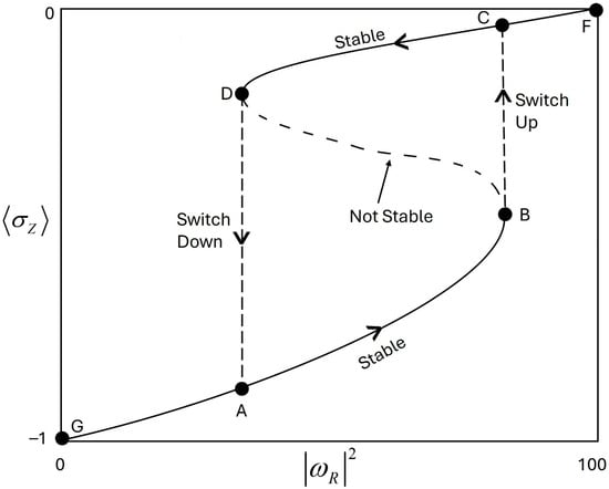
Figure 1. The value of $⟨{\sigma }_z⟩$ as a function of ${\left|{\omega }_R\right|}^2$ is described along the curve GABDCF. The value of $⟨{\sigma }_z⟩$ in the lower curve AB is equal to the value of $⟨{\sigma }_z⟩$ in the upper curve CD for the same light intensity. As the electric field increases (decreases), the system switches from the lower to the upper curve along the dashed line BC (the system switches from the upper to the lower curve along the dashed line DA). The light intensity ${\left|{\omega }_R\right|}^2$ is given in relative units.

Comparing our value obtained for $-\mathrm{Im}\Gamma$, by substituting $\beta ={\displaystyle \frac{4\left|P^2\right|k^3{\lambda }^3}{3\hslash }}$ in our approximate Equation (7), we obtained

$$-\mathrm{Im}\Gamma ={\displaystyle \frac{3\beta n{\lambda }^3}{8{\pi }^2}}={\displaystyle \frac{3n}{8{\pi }^2}}{\displaystyle \frac{4\left|P^2\right|k^3{\lambda }^3}{3\hslash }}={\displaystyle \frac{4\pi }{\hslash }}\left|P^2\right|n$$

(12)

We find that it is equal to the semi-classical value $\epsilon ={\displaystyle \frac{4\pi }{3\hslash }}\left|P^2\right|n$ multiplied by a factor of 3 (it might be that this difference is due to different approximations or due to a small difference in the physical system).

In [9,10], IOB for thin-layer resonant emitters was treated by using similar methods to those presented in our Refs. [4,5]. In particular, the local field effect on Maxwell’s equations is similar. But these works [9,10] add new information on various effects in IOB, e.g., deviations from resonance, inhomogeneous broadening in addition to homogeneous broadening, switching times in IOB, the effect of the real part of the local parameter in addition to its imaginary value, etc.

For coherent radiation transmitted through a long sample, with dimensions very large relative to the wavelength, we use Equations (4) and (5) and study the effect of the spatially varying parameters on the behaviour of the system. The $z$ axis is defined as the direction of propagation of the externally applied field, and the x axis is defined as the direction of polarization. The coefficients $B(i,j)$ are identical to those obtained from classical dipole–dipole interactions [25,26]. We simplify their expressions by assuming that the dipoles of the two atoms in $B(i,j)$ are given as

$${\overrightarrow{p}}_i={\overrightarrow{p}}_j=P\hat{x}$$

(13)

To calculate the interactions of atom $i$ with all other atoms, we separate the interaction into two parts. In the first part, we choose a sphere around the atom $i$ with a radius $r_0$, which is on the order of a wavelength so that in this sphere we can ignore retardation and use the mean field approximation. In the second part, we include the interaction with all other atoms that are not located in this sphere.

In the second part, to calculate its interaction with distant dipoles outside of this sphere, we should consider retardation and propagation effects. For this purpose, it is convenient to describe the expectation values of the atomic operators as continuous variables. We define $⟨{\sigma }_{+0}(r,t)⟩$ and $⟨{\sigma }_z(r,t)⟩$, respectively, as the complex dipole and the inversion of population per unit volume at point $\overrightarrow{r}$. By including both interactions, Equations (4) and (5) can be written in terms of the new variables as

$${\displaystyle \frac{d⟨{\sigma }_z\left(r,t\right)⟩}{dt}}=-{\beta }_1\left[⟨{\sigma }_z⟩+n\right]-\left\{\left[2{\Theta }^{·}\left(r,t\right)+{\omega }_R\right]⟨{\sigma }_{+0}(r,t)⟩+C.C.\right\}$$

(14)

$${\displaystyle \frac{d⟨{\sigma }_{+o}\left(r,t\right)}{dt}}=\left(i\Delta -{\beta }_2\right)⟨{\sigma }_{+o}\left(r,t\right)⟩+\left[\Theta \left(r,t\right)+{\displaystyle \frac{{{\omega }^{·}}_R}{2}}\right]⟨{\sigma }_z⟩$$

(15)

where $\Theta \left(r,t\right)$ is a continuous variable corresponding to the definition of the reaction field $\Theta \left(r,t\right)$ given in Equation (2) and is separated into two parts, $\Theta ={\Theta }_1+{\Theta }_2$, corresponding to the contributions inside and outside the sphere.

By using the mean field approximation for Equations (4) and (5), we express the first part of the cooperative interaction as

$${\Theta }_1\left(r,t\right)=⟨{\sigma }_{+o}\left(r,t\right)⟩{\Gamma }_1/n$$

(16)

After lengthy calculation, given in Appendix B of [4], the value of ${\Gamma }_1$ is given as a function of $R=k{r}_0$, where, by ignoring small oscillations, we obtain

$$⟨\mathrm{Re}{\Gamma }_1⟩\approx 0$$

(17)

$\mathrm{Im}{\Gamma }_1$ is a negative oscillating function of $r_0/\lambda$ with an average value of

$$\mathrm{Im}\Gamma =-{\displaystyle \frac{7}{6}}{\displaystyle \frac{3\beta n{\lambda }^3}{8{\pi }^2}}$$

(18)

After some calculations for ${\Theta }_2$, including retardation and propagation effects, we find that ${\Theta }_2$ is given in the form of the ordinary Maxwell equation in the slowly varying envelop approximation as

$${\displaystyle \frac{1}{c}}{\displaystyle \frac{\mathsf{\partial }{\Theta }_2\left(z,t\right)}{\mathsf{\partial }t}}+{\displaystyle \frac{\mathsf{\partial }{\Theta }_2\left(z,t\right)}{\mathsf{\partial }z}}={\displaystyle \frac{3\pi \beta }{k^3}}⟨{\sigma }_{+o}\left(z,t\right)⟩$$

(19)

By introducing the following definitions into Equations (14)–(16):

$$\begin{array}{l}{{\omega }_R}^{\prime }={\omega }_R+2{{\Theta }_2}^{·}(\overrightarrow{r}),\\ \Gamma \prime =-{{\theta }_1}^{\mathrm{Im}}(\overrightarrow{r})/⟨{\sigma }_{+o}\left(\overrightarrow{r}\right)⟩=-i\left(3/8{\pi }^2\right){\displaystyle \frac{7}{6}}{\lambda }^3\beta \end{array}$$

(20)

these equations can be written in the same form as Equations (4) and (5) for the thin sample, with an imaginary value for $\Gamma$. One should notice that we exchanged the parameters ${\omega }_R$ and $\Gamma$ of the thin sample for ${{\omega }^{\prime }}_R$ and ${\Gamma }^{\prime }$. In the long sample, the effect of ${\Theta }_2$ is to change the effective ${\omega }_R$, but we find that while dipole–dipole interactions with other atoms decrease with increasing distance, the phase factors increase so that this dependence is eliminated and the average value $⟨{{\omega }_R}^{\prime }⟩=⟨{\omega }_R⟩$ [22]. We obtain the important result that the two phases of high and low transitivity may coexist spatially in the material in the long sample, similarly to in the short sample. We obtain the modified Maxwell’s Equations (4)–(15), mainly using $\mathrm{Im}\Gamma$, for both cases (equal to those given in [6]).

2.2. Equations of Motion for Intrinsic Bi-Stability Including Noise Terms

The equations of motion for two-level atoms, including the noise source operators, are given as follows [27,28,29]:

$$\begin{array}{l}d\sigma \left(z,t\right)/dt=-{\beta }_1\left[\sigma \left(z,t\right)+1\right]+\left(\mu /\hslash \right)\left[E^{·}{\sigma }_{+0}(z,t)+E{\sigma }_{-0}(z,t)\right]\\ -{\sigma }_{+0}(z,t)f^{+}(t)-{\sigma }_{-0}(z,t)f^{-}(t)\end{array}$$

(21)

$$\begin{array}{l}d{\sigma }_{+0}/dt=-\left(\mu E/\hslash \right){\sigma }_z(z,t)+i\left[\Delta -\epsilon {\sigma }_z(z,t)\right]{\sigma }_{+o}(z,t)\\ -{\beta }_2{\sigma }_{+o}(z,t)+f^{-}(t){\sigma }_z(z,t)\end{array}$$

(22)

Here ${\beta }_1$ and ${\beta }_2$ are the decay constants of the population inversion and atomic dipole, respectively. $\Delta =\omega -{\omega }_0$ is the deviation from resonance. $\epsilon$ is the frequency renormalization, defined previously as $\mathrm{Im}\Gamma$. In the above analysis, we used the equations of motion under stationary conditions, where the expectation values of the noise sources vanished. Here, the noise sources are added to the external field with the properties

$$⟨f^{+}(t)f^{-}(t\prime )⟩={\beta }_1\delta (t-t) ⟨f^{+}(t)f^{+}(t\prime )⟩=⟨f^{-}(t)f^{-}(t\prime )⟩=⟨f^{-}(t)f^{+}(t\prime )⟩=0$$

(23)

where $\beta$ is the spontaneous decay constant.

Through adiabatic elimination of ${\sigma }_{+0}$ and ${\sigma }_{-0}$ from Equation (22), we obtain

$$\begin{array}{l}d{\sigma }_z=\left(-{\beta }_1\left[\sigma \left(z,t\right)+1\right]-{\displaystyle \frac{2{\left|{\omega }_R\right|}^2{\sigma }_z{\beta }_2}{{\left(\Delta -\epsilon {\sigma }_z\right)}^2+{\beta }_2^2}}\right)dt\\ +\left({\displaystyle \frac{{\omega }_R{\sigma }_z}{i\left(\Delta -\epsilon {\sigma }_z\right)-{\beta }_2}}d{F}^{+}+{\displaystyle \frac{{{\omega }_R}^{·}\sigma z}{-i\left(\Delta -\epsilon {\sigma }_z\right)-{\beta }_2}}d{F}^{-}\right)\end{array}$$

(24)

where ${\omega }_R={\displaystyle \frac{\mu E}{\hslash }}$ is the Rabi frequency of the applied external field. We defined here the stochastic variables $d{F}^{+}$ and $d{F}^{-}$ by the equations

$${\displaystyle \frac{d{F}^{+}}{dt}}=f^{+}(t) ; {\displaystyle \frac{d{F}^{-}}{dt}}=f^{-}(t)$$

(25)

We have the corresponding relations:

$$\begin{array}{l}⟨d{F}^{+}\left(t\right)d{F}^{-}\left(t\prime \right)⟩={\beta }_{1}dt ; \\ ⟨d{F}^{+}\left(t\right)d{F}^{+}\left(t\prime \right)⟩=⟨d{F}^{-}\left(t\right)d{F}^{-}\left(t\prime \right)⟩=⟨d{F}^{-}\left(t\right)d{F}^{+}\left(t\prime \right)⟩=0\end{array}$$

(26)

We transform Equation (24) into a Fokker–Planck equation by using the corresponding methods from the literature [28,29] for the inversion of population probability $f({\sigma }_z)$ as a function of the parameters ${\left|{\omega }_R\right|}^2$ $\Delta ,\epsilon ,{\beta }_1,{\beta }_2$:

$$\begin{array}{l}{\displaystyle \frac{\mathsf{\partial }f\left({\sigma }_z\right)}{\mathsf{\partial }t}}=-{\displaystyle \frac{\mathsf{\partial }}{\mathsf{\partial }{\sigma }_z}}\left[\left(-{\beta }_1\left({\sigma }_z+1\right)-{\displaystyle \frac{2{\left|{\omega }_R\right|}^2{\sigma }_z{\beta }_2}{{{\beta }_2}^2+{\left(\Delta -\epsilon {\sigma }_z\right)}^2}}\right)f\left({\sigma }_z\right)\right]\\ +{\displaystyle \frac{1}{2}}{\displaystyle \frac{{\mathsf{\partial }}^2}{\mathsf{\partial }{\sigma }_z^2}}\left({\displaystyle \frac{{\left|{\omega }_R\right|}^2{{\sigma }_z}^2{\beta }_1}{{{\beta }_2}^2+{\left(\Delta -\epsilon {\sigma }_z\right)}^2}}f({\sigma }_z)\right)\end{array}$$

(27)

We represent the drift term $A\left({\sigma }_z\right)$ and the diffusion coefficient $B\left({\sigma }_z\right)$ as

$$\begin{array}{l}-A({\sigma }_z)=-{\beta }_1\left({\sigma }_z+1)\right)-{\displaystyle \frac{{\left|{\omega }_R\right|}^2{\sigma }_z{\beta }_2}{{{\beta }_2}^2+{\left(\Delta -\epsilon {\sigma }_z\right)}^2}}\\ B({\sigma }_z)={\displaystyle \frac{{\left|{\omega }_R\right|}^2{{\sigma }_z}^2\beta 1}{{{\beta }_2}^{2}2+{\left(\Delta -\epsilon {\sigma }_z\right)}^2}}\end{array}$$

(28)

Usually, we solve the bi-stability effects under steady-state conditions, where the expectation values of the noise sources vanish. The solutions of Equation (27) generalize such analysis, where each point in the bi-stability diagram is diffused into a certain broadened function, which depends on the ratios of the above parameters. In cases in which these noise sources are very large, any bi-stability observation [28] might be avoided. Also, cooperative luminescence effects might be very large relative to the dipole–dipole interactions. The solutions to Equation (27) might help in treating various bi-stability effects, e.g., calculations of average passage times between the two metastable states in IOB [28].

3. Results for Optical Intrinsic Bi-Stability in Excited Atomic Dimers, with Ion Pairs and Up-Conversion with Intermediate Virtual Level

Mirrorless intrinsic bi-stability in dense media was realized in a set of experiments performed by Hehlen and her colleagues [16,17,18,19,20]. The two-level density matrix was extended to incorporate new contributions expected from strong dipolar interactions among excited states. Pertinent to a variety of systems, intrinsic bi-stability was predicted to depend on a combination of ground- and excited-state coupling, and this phenomenon was observed in the cooperative pair luminescence of dimeric compounds. The excitation energy is partitioned between the excited atom and a ground state collision partner at a rate that is bilinear to their respective intensities and therefore nonlinear with respect to occupation numbers. The reverse process, called cooperation up-conversion, can be efficient and is the process responsible for the observed IOB. The model incorporates the cooperative dynamics of two three-level atoms, which gives rise to (a) cross relaxation and (b) pair up-conversion. The dynamics of interest can be treated with a two-level pair model of cooperative processes, which introduces local field corrections to the optical polarization. Of the three states, one participates as an intermediate virtual state. Its role as a virtual state can be preserved within the framework of the two-level model.

Intrinsic optical bi-stability was measured in excited atomic states, belonging to the ‘Lanthanide’ chemical elements [16,17,18,19,20,21,22]. These series of elements include 14 chemical elements with atomic numbers 57–70, from lanthanum through to ytterbium. In the periodic table, they fill the 4f orbitals. The electronic configuration of a ytterbium atom is described as.

Yb: $1s^{2}2s^{2}2p^{6}3s^{2}3p^{6}4s^{2}3d^{10}4p^{6}5s^{2}4d^{10}5p^{6}6s^{2}4f^{14}$, with atomic number 70, and a thulium atom has an atomic number of 69. $Y{b}^{3+}$ and $T{m}^{3+}$ elements have an ionized electron and a valence of 3. Intrinsic optical bi-stability has been observed in dimeric compounds [16,17,18,19,20,21,22] through the up-conversion process. In [16,17,18,19,20], the two-level density matrix was extended to incorporate the contribution expected from strong dipole interactions among excited states. Excitation energy is partitioned between the excited atom and a ground state collision partner at a rate which is bilinear in their respective densities and therefore nonlinear with respect to occupation probabilities. The equations of motion for intrinsic bi-stability were developed for the off-diagonal coherence ${\sigma }_{21}$ and inversion of population ${\sigma }_3$ of the density matrix [16].

$$\begin{array}{l}{\displaystyle \frac{d{\sigma }_{21}}{dt}}=-i\left(\Delta +\epsilon {\sigma }_3\right){\sigma }_{21}-{\displaystyle \frac{1}{2}}i\Omega {\sigma }_3-{\Gamma }_{21}{\sigma }_{21} ; 2\left({\rho }_{22}-{\rho }_{11}\right)={\sigma }_3 ; {\rho }_{12}={\left({\rho }_{21}\right)}^{·}\end{array}$$

(29)

$${\displaystyle \frac{d{\sigma }_3}{dt}}=-i2\Omega \left({\sigma }_{21}-{{\sigma }^{·}}_{21}\right)-\gamma \left({\sigma }_3-{\sigma }_{30}\right)-\alpha {\left({\sigma }_3-{\sigma }_{30}\right)}^2 ;$$

(30)

where $\epsilon$ is the absolute value of $\Gamma$ given by Equation (7). The factor of 2 accounts for the two excited atoms that decay for each cooperative up-conversion event. The coupling between ${\sigma }_3$ and ${\sigma }_{21}$ is described in Figure 2. This figure describes the up-conversion process by which the excitation reaches a level of $\left|3\right.⟩$, and decay is described by linear and nonlinear terms. The IOB detuning of light from the resonance frequency is denoted by $\Delta$, and $\Omega$ is the Rabi frequency:

$$\Delta =\omega -{\omega }_0 ; \Omega =\mu E/\hslash$$

(31)

${\sigma }_{21}$ is the off-diagonal matrix element. Experimental observations of bi-stability luminescence from $Y{b}^{3+}$ pairs, in various crystals, confirm the theoretical predictions and have interesting implications for local field effects in solids and dense ultracold gases. Both theory and experimental evidence show that increasing the coupling between $Y{b}^{3+}$ dimers enhances the observability of IOB. The bi-stability region becomes narrower and shifts to a lower excitation energy with increasing temperatures and concentration. The off-diagonal density matrix element ${\sigma }_{21}$ is produced by the external EM field at frequency $\omega$ with detuning $\omega -{\omega }_0$. The upper-level density matrix includes two excited atoms that decay with the ordinary term $-\gamma ({\sigma }_3-{\sigma }_{30})$ and the quadratic decay term $-\alpha {({\sigma }_3-{\sigma }_{30})}^2$, where for low temperatures the thermal occupation of the excited state is given by ${\sigma }_{30}=-1$. The bi-stability’s effective two-level dynamics in two rare earth excited ionic dimers are described in Figure 2.

In ordinary two-level intrinsic bi-stability, noise sources appear as additional terms that replace the external field and thus affect the bi-stability. In Equation (8), we use the steady-state approximation for the complex dipole, in which noise is neglected [4]. But such noise terms lead to rapid dephasing of the complex dipole, leading to incorrect adiabatic elimination of the complex dipole. The observation of bi-stability is dependent on the strength of the noise terms of the complex dipole relative to the strength of the dipole–dipole interactions. The situation is quite different in the case of excited rare earth crystals. As can be observed in Figure 2, the intermediate level is virtual, and through up-conversion, state 2 is moved to state 3. The crucial point is that the noise terms mainly affect population inversion at the third level and not in the complex dipole. Mathematically, this means that, in Equation (29), ${\Gamma }_{21}$ can be neglected relative to the strong dipole–dipole interaction occurring in rare earth excited crystals. This might be why intrinsic bi-stability in crystalline dimers has better observability.

In steady-state conditions, the time derivatives in Equation (29) are equal to zero. This yields

$${\sigma }_{21}={\displaystyle \frac{-\left(1/2\right)i\Omega {\sigma }_3\left[\Gamma -i\left(\Delta +\epsilon {\sigma }_3\right)\right]}{{\Gamma }^2+{\left(\Delta +\epsilon {\sigma }_3\right)}^2}}$$

(32)

From Equation (32), we obtain

$${\sigma }_{21}-{{\sigma }^{·}}_{21}={\displaystyle \frac{-i\Omega {\sigma }_3\Gamma }{{\Gamma }^2+{\left(\Delta +\epsilon {\sigma }_3\right)}^2}}$$

(33)

Assuming $d{\sigma }_3/dt=0$ in Equation (29) and substituting Equation (33) into this equation, we obtain

$$\left[\gamma \left({\sigma }_3-{\sigma }_{30}\right)+\alpha {\left({\sigma }_3-{\sigma }_{30}\right)}^2\right]\left({\Gamma }^2+{\left(\Delta +\epsilon {\sigma }_3\right)}^2\right)=-\Omega {\sigma }_3\Gamma$$

(34)

Under the approximation $\alpha =0$, Equation (34) is equivalent to the cubic Equation (11), where the notations ${\beta }_1,{\beta }_{2,}⟨{\sigma }_z⟩+1,\mathrm{Im}\Gamma ,{\left|{\omega }_R\right|}^2$ are changed to the notations used in Equation (32) in [16]: $\gamma , \Gamma , {\sigma }_3-{\sigma }_{30}, \epsilon , \Omega$, respectively. The quartic Equation (34), when $\alpha$ and $\epsilon$ are not zero, results in nonlinear dynamics solutions that are multi-valued and describe the full features of bi-stability in the population inversion. Various figures have been plotted to describe bi-stability properties in crystalline dimer systems [16,17,18,19,20,21,22].

Figure 2. A two-level theoretical model of the cooperative dynamics is related to levels $\left|1\right.⟩$ and $\left|3\right.⟩$, where level $\left|2\right.⟩$ is virtual. The curved arrows show non-radiative transitions through collisions. The equations of motion for ${\sigma }_3$ and ${\sigma }_{21}$ are described in Equations (29) and (30) [16]. The decay from level $\left|3\right.⟩$ is described by linear and quadratic terms $-\gamma \left({\sigma }_3-{\sigma }_0\right)-\alpha {\left({\sigma }_3-{\sigma }_0\right)}^2$, where for low temperatures ${\sigma }_0=-1$, as this is the lowest value of $\sigma$.

4. Discussion and Conclusions

The idea of making “mirrorless” bistable devices, including local field corrections (LFC) to create the bi-stability, was developed in a series of papers by Bowden and his colleagues [1,2,3,4,5,6,7]. Several additional properties of such systems were developed further by other authors [8,9,10,11]. In the present paper, I discussed physical schemes of two-level systems in which bi-stability might be realized and explained its observability in excited crystalline dimers [16,17,18,19,20,21,22].

Mirrorless intrinsic bi-stability in crystalline dense media was realized in experiments performed by Hehlen and colleagues [16,17,18,19,20]. The observed process is described in Figure 2, involving up-conversion in a three-level system, in which the intermediate level is virtual. The equations of motion are developed for ${\sigma }_{21}$ and ${\sigma }_3$, where the interaction is between ionic pairs of $Y{b}^{3+}$. Similar observations in ytterbium atoms were obtained in rare earth ion pairs in solids [30]. We therefore also expect observable intrinsic bi-stability in other solid systems. It was claimed, however, that excitonic effects cause unstable spatially uniform solutions and drastically decrease the existence range of intrinsic optical bi-stability [18,20]. The cooperative luminescence in ytterbium-doped $CsCdB{r}_3$ was calculated to be in agreement with experiments [30]. We found that such cooperative effects mitigate intrinsic optical bi-stability.

The decay constant of ${\sigma }_3$ in the intrinsic bi-stability experiments [16,17,18,19,20,21,22] was obtained as $-\gamma \left({\sigma }_3-{\sigma }_{30}\right)-\alpha {\left({\sigma }_3-{\sigma }_{30}\right)}^2$, where $\gamma$ and $\alpha$ are constants. Due to nonlinear decay, $⟨{\sigma }_3⟩$ written as function of ${\left|{\omega }_R\right|}^2$ is a quartic equation. Intrinsic optical bi-stability was demonstrated in Refs. [16,17,18,19,20,21,22] by plotting ${({\sigma }_3-{\sigma }_{30})}^2$ (which is proportional to the luminescence light intensity) as function of the excitation intensity (W ${\mathrm{cm}}^{-2}$). The magnitude of $\mathrm{Im}\Gamma$ [4] (defined in [6] as $\epsilon$) relative to other parameters is a critical value for obtaining intrinsic bi-stability. The bi-stable region becomes narrower and shifts to lower excitation energies at higher temperatures. The optical bi-stability described in the present work is intrinsic and not the result of external feedback.

The results obtained in previous work [4] were obtained using steady-state conditions. But in cases for which the time dependence of $d{\sigma }_z/dt$ and $d{\sigma }_{+0}/dt$ is also important, we need to add Langevin noise terms, as follows from the fluctuation–dissipation theorem [27]. The equations of motion for two-level atoms, including the noise source operators, are given in Equations (21) and (22) [28]. By following general quantum statistics methods [28,29], these equations were transformed into the Fokker–Planck Equation (27), which included the drift term $A\left({\sigma }_z\right)$ and the diffusion coefficient $B\left({\sigma }_z\right)$. While there is a lot of literature on non-Markovian processes [31], we used a special procedure through which the noise terms in the complex dipole are neglected and the noise only exists in the population terms related to the Fokker–Planck equation.

Such a procedure is only justified for three-level atoms where the second level is virtual, and the noise only exists in the population of the third level. So this explains why bi-stability was not observed in an ordinary two-level system, as one cannot neglect the noise terms for the complex dipole in an ordinary two-level system as this leads to dephasing of the complex dipole. The conclusion is that the noise terms should only be included for a three-level system in which the second level is virtual.

One may also use this simplification of noise terms to reduce complex dipole noise in other cases, e.g., in the field of quantum computation [32], in which reducing quantum noise is very important.

In conclusion, we have explained the differences between a simple two-level system and systems of rare earth materials enabling bi-stability observation. These rare earth materials [33] have many applications, including for health problems, as described in a recent review [34]. The present analysis provides new physical insights in this field.

References

- Bowden, C.M.; Sung, C.C. First-and second-order phase transitions in the Dicke model: Relation to bi stability. Phys. Rev. A 1979, 19, 2392–2401. [Google Scholar] [CrossRef]
- Hopf, F.A.; Bowden, C.M.; Louisell, W.H. Mirrorless optical bi stability with the use of the local field correction. Phys. Rev. A 1984, 29, 2591–2596. [Google Scholar] [CrossRef]
- Hopf, F.A.; Bowden, C.M. Heuristic stochastic model of mirrorless optical bi stability. Phys. Rev. A 1985, 32, 268–275. [Google Scholar]
- Ben-Aryeh, Y.; Bowden, C.M.; England, J.C. Intrinsic optical bi stability in collection of spatially distributed two-level atoms. Phys. Rev. A 1986, 34, 3917–3926. [Google Scholar] [CrossRef]
- Ben-Aryeh, Y.; Bowden, C.M.; Englund, J.C. Longitudinal special first-order phase transition in a system of coherently driven, two-level atoms. Opt. Comm. 1987, 61, 147–150. [Google Scholar]
- Bowden, C.M.; Dowling, J.P. Near-dipole-dipole effects in dense media: Generalized Maxwell-Bloch equations. Phys. Rev. A 1993, 47, 1247–1251. [Google Scholar] [CrossRef] [PubMed]
- Crenshaw, M.E.; Bowden, C.M. Local-field effects in a dense collection of two-level atoms embedded in a dielectric medium: Intrinsic optical bi-stability enhancement and local cooperative effects. Phys. Rev. A 1996, 53, 1139–1142. [Google Scholar] [PubMed]
- Goldstone, J.A.; Garmire, E. Intrinsic optical bi stability in nonlinear media. Phys. Rev. Lett. 1984, 53, 910–912. [Google Scholar]
- Benedict, M.G.; Malysshev, V.A.; Trifonov, E.D.; Zaitsev, A.I. Reflection and transmission of ultrashort light pulses through a thin resonant medium: Local field effects. Phys. Rev. A 1991, 43, 3845–3853. [Google Scholar] [CrossRef]
- Malikov, R.F.; Malyshev, V.A. Optical bi stability and hysteresis of a thin layer of resonant emitters: Interplay of in homogenous broadening of the absorption line and the Lorentz local field. Opt. Spectrosc. 2017, 122, 955–963. [Google Scholar]
- Yoon, Y.-K.; Bennink, R.S.; Boyd, R.W.; Sipe, J.E. Intrinsic optical bi stability in a thin layer of nonlinear optical material by means of local field effects. Opt. Comm. 2000, 179, 577–580. [Google Scholar]
- Gibbs, H.M. Optical Bistability. In Controlling Light with Light; Academic Press: New York, NY, USA, 1980. [Google Scholar]
- Bowden, C.M.; Ciftan, M.; Robl, R. Optical Bi Stability; Plenum: New York, NY, USA, 2012. [Google Scholar]
- Joshi, A.; Xiao, M. Controlling Steady-State and Dynamical Properties of Atomic Bi Stability; World Scientific: Singapore, 2012. [Google Scholar]
- Lugiato, L.A., II. Theory of optical bi stability. Prog. Opt. 1984, 21, 69–216. [Google Scholar]
- Hehlen, M.P.; Gudel, H.U.; Shou, Q.; Rai, J.; Rai, S.; Rand, S.C. Cooperative bi stability in dense, excited atomic systems. Phys. Rev. Lett. 1994, 73, 1103–1106. [Google Scholar] [PubMed]
- Hehlen, M.P.; Gudel, H.U.; Shou, Q.; Rand, S.C. Cooperative optical bi stability in the system CS3Y2Br9:10%Yb3+. J. Chem. Phys. 1996, 104, 1232–1244. [Google Scholar]
- Luthi, S.R.; Hehlen, M.P.; Riedener, T.; Gudel, H.U. Excited-state dynamics and optical bi stability in the dimer system Cs3Lu2Br9:Yb3+. J. Lumin. 1998, 76–77, 447–454. [Google Scholar]
- Hehlen, M.P.; Kuditcher, A.; Rand, S.C.; Luthi, S.R. Site-selective, intrinsically bi stable luminescence of Yb3+ ions pairs in CsCdBr3. Phys. Rev. Lett. 1999, 82, 3050–3053. [Google Scholar]
- Hehlen, M.P.; Guedel, H.U. Optical Spectroscopy of the Dimer System Cs3Yb2Br9. ChemInform 1993, 98, 1768–1799. [Google Scholar] [CrossRef]
- Kuditcher, A.; Hehlen, M.P.; Florea, C.M.; Winick, K.W.; Rand, S.C. Intrinsic bi stability of luminescence and stimulated emission in Yb- and Tm-doped glass. Phys. Rev. Lett. 2000, 84, 1898–1901. [Google Scholar]
- Chen, Y.-H.; Horwath, S.P.; Longdell, J.J.; Zahng, X. Optically unstable phase from ion-ion interactions in an erbium doped crystal. Phys. Rev. Lett. 1994, 196, 371–376. [Google Scholar] [CrossRef]
- Guillot-Noel, O.; Binet, L.; Gourier, D. Towards intrinsic optical bi stability of rare earth ion pairs in solids. Chem. Physic Lett. 2001, 344, 612–618. [Google Scholar]
- Yudson, V.I.; Reineker, P. Excitons effects in dense media: Breakdown of intrinsic optical bi stability. Phys. Lett. A 1995, 196, 371–376. [Google Scholar] [CrossRef]
- Milonni, P.W.; Knight, P.L. Retardation in the resonant interaction of two identical atoms. Phys. Rev. A 1974, 10, 1096. [Google Scholar] [CrossRef]
- Ben-Aryeh, Y.; Bowden, C.M. Mirrorless optical bi stability in a spatially distributed collection of two-level systems. Opt. Commun. 1986, 59, 224–228. [Google Scholar] [CrossRef]
- Kubo, R. The fluctuation-dissipation theorem. Rep. Prog. Phys. 1966, 29, 255. [Google Scholar] [CrossRef]
- Ben-Aryeh, Y.; Bowden, C.M. Quantum noise effects in intrinsic optical bi stability of a system of interacting two-level atoms. Opt. Commun. 1989, 72, 335–340. [Google Scholar] [CrossRef]
- Song, T.T. Random Differential Equations in Science and Engineering; Academic Press: New York, NY, USA, 1973. [Google Scholar]
- Goldner, P.; Pelle, F.; Meichenin, D.; Auzel, F. Cooperative luminescence in erbium-doped CsCDBr3. J. Lumin. 1997, 71, 137–150. [Google Scholar] [CrossRef]
- Vacchini, V.; Breuer, H.-P. Exact non-Markovian decay of a qubit. Phys. Rev. A 2010, 81, 042103. [Google Scholar]
- Nielsen, M.A.; Chuang, I.L. Quantum Computation and Quantum Information; Cambridge University Press: New York, NY, USA, 2010. [Google Scholar]
- Olden, N.E.; Coplen, T. The Periodic Table of the Elements. Chem. Int. 2004, 26, 8–9. [Google Scholar] [CrossRef]
- Wang, X.; Wang, F.; Yan, L.; Gao, Z.; Yang, S.; Su, Z.; Chen, W.; Li, Y.; Wang, F. Adverse effects and underlying mechanism of rare earth elements. Environ. Health 2025, 24, 31. [Google Scholar] [CrossRef]
Disclaimer/Publisher’s Note: The statements, opinions and data contained in all publications are solely those of the individual author(s) and contributor(s) and not of MDPI and/or the editor(s). MDPI and/or the editor(s) disclaim responsibility for any injury to people or property resulting from any ideas, methods, instructions or products referred to in the content. |
© 2025 by the author. Licensee MDPI, Basel, Switzerland. This article is an open access article distributed under the terms and conditions of the Creative Commons Attribution (CC BY) license.