Abstract
Suspended conveyor belts are widely used in mining, including in systems with non-contact support such as magnetically suspended conveyors, where the maximum admissible linear mass of the loaded belt determines the required supporting forces. This paper presents a method for estimating the upper limit of the linear mass of a suspended belt for a given belt width and bulk material. Several cross-sectional configurations are analysed, and analytical expressions for the bulk cross-sectional area under limiting fill are derived. A numerical search over the troughing radius is then performed to find the radius that maximises the cross-sectional area and to select the configuration that provides the largest area. For this configuration, the extremum condition leads to a transcendental equation; so, symbolic regression with the PySR package is used to obtain an explicit approximation for the radius that maximises the area as a function of belt width and angle of repose. Substituting this expression into the standard formula for linear mass yields a closed-form estimate of the maximum admissible linear mass. Numerical examples show good agreement with the optimisation results and indicate that the formula is suitable for preliminary design of suspended and magnetically suspended belt conveyors.
1. Introduction
Conveyor systems play a pivotal role in the mining industry, enabling the continuous transportation of ore and overburden over long distances [1]. In light of escalating requirements for productivity and process sustainability, the enhancement of conveyor systems has become a strategic priority [2].
One promising avenue for advancing conveyor transport is the development of suspended-belt conveyors, in which the belt is supported by hangers, ropes, or other discretely spaced elements instead of conventional idler sets [3]. One variety of suspended conveyors is the conveyor with magnetic suspension of the belt [4]. Their operating principle relies on magnetic forces that support the belt without mechanical contact with structural supports [5]. This is achieved by generating a magnetic field that compensates the weight of the belt and the conveyed material [6]. The principal advantage of such systems is the reduction in friction, which directly lowers energy losses, increases the overall efficiency of the conveyor, and diminishes component wear. Eliminating belt–support contact removes the need for idler rollers, reduces friction in the support zone, and extends equipment service life [7].
In magnetically levitated conveyors, the suspended belt passes above a series of discretely spaced magnetic modules (with permanent magnets or electromagnets) that create a supporting magnetic field and hold the belt within a prescribed air gap. The magnets are placed either under the belt edges or beneath its central part, and the spacing between modules defines the distance between neighboring suspension points. In such a configuration, each span of the suspended belt must sustain its own linear mass of belt and load without losing stability and without exceeding the allowable deflections and air gap. For magnetically levitated conveyors [8,9], as for other suspended-belt systems, one of the key design characteristics is the maximum permissible linear mass of the loaded belt. The stability of the suspended belt and the levitation margin are directly governed by the balance between the available lifting force and the total belt-and-load mass per unit length. Exceeding the allowable linear mass may lead to loss of stability or belt overturning, which results in shutdowns of conveying and potential equipment damage. Therefore, a method for calculating the maximum linear mass is required already at the preliminary design stage of such systems.
In most existing conveyor design methods, the problem of determining the limiting load and capacity is treated for belt conveyors with idler sets. Classical approaches are based on models of the cross-section of a troughed belt on idler supports [10,11,12]. In these models, the idler geometry (troughing angles, roller arrangement) is prescribed, and analytical relationships are derived for the cross-sectional area of the bulk load, the utilization factor of the belt width, the permissible fill level and, consequently, the conveying capacity and the load on the belt. In a number of standards and handbooks these relationships are provided in the form of ready-made formulas and charts, which makes it possible to estimate the limiting mass of the load and the belt loading for a given idler scheme.
However, for suspended and magnetically suspended conveyors [13,14] these approaches face fundamental limitations. First, in classical models the cross-sectional shape is rigidly determined by the idler geometry and is not treated as the result of maximizing the cross-sectional area. Second, the support spacing is not explicitly linked to the shape of the cross-section. Third, in many works the mass of the belt and the bulk per unit length is introduced as an input parameter, whereas the problem of determining the maximum permissible linear mass for a given belt width and material properties is not formulated explicitly.
In suspended-belt systems the cross-sectional shape is not the same as in the presence of idlers; instead, it is governed by the spacing between supporting elements and by the properties of the bulk material. As a result, the classical formulas for idler-supported conveyors do not provide a direct answer to the question of what maximum linear mass can be realized for a suspended belt of a given width and material under an admissible cross-sectional shape. This motivates the development of a method for calculating the ultimate attainable linear mass specifically for suspended belt conveyors, including those with magnetic levitation, as well as a compact analytical relationship linking the troughing parameters to this limit under realistic cross-sectional shapes of the bulk material.
Thus, the novelty of the present study lies in transferring the problem of determining the maximum linear mass from the context of idler-supported conveyors to the context of a suspended belt, where the cross-sectional shape and suspension parameters are treated as design variables. The proposed methodology is tailored to the suspended-belt type and is intended for integration into the design calculations of magnetically levitated conveyors while also being applicable to other suspended-belt systems.
The objective of this study is to develop a methodology for determining the maximum attainable linear mass of a loaded suspended conveyor belt for a given belt width and bulk-material properties [15]. The approach is based on analyzing the transverse geometry of the material layer on the belt, determining the troughing parameters at which the cross-sectional area attains its maximum, and constructing a compact analytical model that combines the bulk mass and the belt mass into a single expression for the maximum permissible linear mass.
A number of studies indicate that the configuration and operating modes of cutting-and-loading equipment directly affect the stability of material feed onto the conveyor, contact loads, and maintenance requirements. It has been shown that optimizing the layout of modules and their interfaces with conveying systems reduces wear of contact units and stabilizes conveying regimes [16]. In parallel, logistics chains are being digitalized: sensor networks, streaming analytics, and predictive maintenance provide end-to-end monitoring of conveyors, control of load distribution, and early detection of adverse operating regimes [17]. For magnetically levitated conveyors, these results are particularly important, because maintaining the prescribed air gap and balancing the lifting force against the linear mass require embedded measurements and real-time, data-driven control loops.
Another important aspect is the formation of the material stream on the belt in the loading zone. Experimental studies show that targeted design refinements of loading devices (for example, the use of an auxiliary blade on a shearer) improve cleanup and make the discharge stream more uniform, reducing impact overloads and fluctuations in the fill factor as material is transferred onto the belt [18]. For magnetic-levitation systems, this directly increases the stability margin of the suspended belt and reduces the likelihood of air-gap collapse or overturning by lowering peaks in the required lifting force per unit length.
Within this study, several cross-sectional configurations characteristic of suspended belts (configurations a–d) are considered. For each configuration, analytical expressions are derived for the cross-sectional area of the bulk load at limiting fill. A numerical search is then performed on a grid of belt widths and angles of repose to find the troughing radius at which the cross-sectional area is maximized and to identify the configuration that provides the largest area. It is shown that, in the range of parameters considered, one of the configurations yields the maximum area, and the corresponding extremum condition leads to a transcendental equation for the troughing radius that does not admit a simple closed-form solution.
To obtain an expression suitable for practical design, symbolic regression with the PySR package is applied to represent the optimal troughing radius as a function of belt width and angle of repose. Based on numerically determined values of the radius that maximize the cross-sectional area, a compact explicit approximation for the troughing radius is constructed. Substituting this expression into the standard formula for the linear mass, which accounts for the bulk density and the areal mass of the belt, yields a closed-form analytical expression for the maximum permissible linear mass of the loaded suspended belt.
The main results of this study are as follows: analytical expressions for the cross-sectional area at limiting fill are obtained; the configuration and troughing radius that provide the maximum area are determined numerically; using symbolic regression in PySR, an explicit approximation is constructed for the troughing radius at which the area is maximal; and, on the basis of this approximation, a closed-form expression is derived for the maximum permissible linear mass of a suspended belt, suitable for preliminary design of suspended and magnetically levitated conveyors.
2. Materials and Methods
2.1. Factors Governing the Maximum Mass per Unit Length
Mass per unit length is the total mass per one meter of the conveyor belt, comprising the mass of the belt itself and the mass of the conveyed material over that segment. Maximizing the material mass on the belt requires simultaneously: maximizing the cross-sectional area of the bulk load, , and achieving a high fill factor, .
The cross-sectional area is determined by the belt’s troughing geometry—namely, the belt width l, the suspension spacing AB, and the troughing radius R. Forming the belt into a trough increases carrying capacity relative to a flat belt [11,12,19]. The fill factor k represents the fraction of the available volume that is actually occupied by material; it depends on the angle of repose , moisture content, particle-size distribution and particle shape, and the loading conditions [20,21,22]. For dry, free-flowing bulk materials, typically reaches 0.85–0.95, whereas for sticky or coarse, blocky materials it is commonly 0.6–0.7 or lower.
The relationship between geometry and the mass per unit length is given by:
where —linear mass, —is the bare-belt mass per unit length (without payload), —is the bulk density of the conveyed material, —is the fill factor, —is the cross-sectional area of the bulk. Throughout all formulas, the angle is expressed in radians (tabulated values given in degrees are converted to radians prior to use).
2.2. Cross-Sectional Geometry of the Bulk Load on the Belt
The cross-sectional [23] shape (Figure 1) is governed by the interplay among the belt width l, the suspension spacing AB, and the troughing radius R, and can be realized in four configurations, a–d [24,25].
Figure 1.
Variants of the cross-sectional shape of the load on the belt: (a)—flat belt; (b)—belt with a trough smaller than a semicircle; (c)—belt with a semicircular trough and a vertical section; (d)—belt with a semicircular trough. Notation: l—belt width; AB—suspension spacing; R—troughing radius; d—arc length between the suspensions O—apex of the bulk material heap, U—center of the belt trough circle.
- a:l = AB (flat belt (no troughing));
- b:l > AB, AB < 2R, l < 2R d = l; the arc length between the suspensions equals the belt width
- c:l > AB, AB = 2R, l > 2R, d < l;
- d:l > AB, AB = 2R, l > 2R, d = l.
Among the cross-sectional configurations (a–d), we sought the shape that maximizes Sg under limiting fill (accounting for the angle of repose j). For each variant, closed-form expressions Sg(a–d)(R) were derived. The optimal radius Ropt was obtained from the first-order condition ∂Sg/∂R = 0 and verified as a maximum within the admissible domain. A comparative summary Sg,max across a–d is provided in (Table 1).

Table 1.
Comparison of the Maximum Cross-Sectional Area of the Bulk Load Across Configurations.
The optimal configuration is defined by the maximization of the cross-sectional area under limiting fill, i.e.,:
where ()—denotes the admissible set of radii , dictated by the geometry (Figure 1) and by design constraints (e.g., the relationships among AB, , ). Throughout all equations, the angle is expressed in radians.
2.3. Software Environment and Reproducibility
To obtain Ropt employed a one-dimensional optimization with multiple initial guesses (multi-start robust search) to avoid entrapment in local extrema; candidate solutions that violated geometric constraints (e.g., AB ≤ 2R for the relevant configurations) were rejected. For verification, we also computed Sg(R) profiles on an R—grid and cross-checked the locations of the maxima (Figure 2 and Figure 3).
Figure 2.
Derivative of the area with respect to the troughing radius.
Figure 3.
Dependence of Sg(R).
Only for configuration b (troughing less than a semicircle) does the optimality condition lead to a transcendental equation that does not admit a simple closed-form solution for . For configurations a, c, and d, the maximizing radius and the corresponding maximum area can be obtained analytically; so, symbolic regression is not required for them. Consequently, PySR was applied exclusively to the dataset for configuration b in order to replace the numerical solution with a compact explicit formula suitable for engineering calculations.
For each pair, maximum troughing radius for configuration B was determined by numerically solving the transcendental equation for the maximum bulk cross-sectional area , whose derivation is presented in Section 3 (Results). Thus, the dataset used in the subsequent symbolic regression consists of the values obtained from this numerical solution of the cross-sectional-area maximization problem.
A data table comprising 1100 observations with three columns:
R_opt, l_1, j_1. Ranges:
l1∈[100, 10,000] (mm);
j1∈[0.1745, 1.0472] rad (≈10–60°);
—maximum troughing radius.
Missing or invalid entries were removed, yielding a final sample of 1100 rows. The dataset was randomly partitioned into training and test subsets in an 80/20 split using random_state = 42.
To approximate the mapping Ropt = f(l,j) employed PySR (SymbolicRegression.jl). The operator set comprised:
{+, −, ×, ÷, pow, √, exp, log, square, cube, inv}, where inv(x) = 1/x. Training employed a complexity cap maxsize = 20 and a parsimony penalty parsimony = 10.0. The evolutionary search settings were: niterations = 100, populations = 10, population_size = 100, and a wall-time limittimeout_in_seconds = 600. Variable names were—l, j. Model quality was assessed on the test set using Ropt In addition, physical plausibility was verified via monotonicity checks: Ropt increases with l at fixed j and decreases with j at fixed l.
Approximation quality was evaluated on the test set, yielding R2 ≈ 0.999 and a typical relative error in Ropt— < 0.1%. In addition, we verified dimensional consistency (unit balance) and scale homogeneity, checked monotonicity with respect to l and j, and assessed robustness via a stress test that removed 5–10% of the data (stress-test).
Python [3.13.7], PySR [1.5.9], NumPy [2.3.2], Pandas [2.3.2], Scikit-learn [1.7.1]; PySR interfaced Julia [1.11.6]. Randomness was controlled by setting the pseudo-random seed = 42. The complete training code and data-preparation scripts are available in the repository [26].
3. Results
3.1. Computation of the Maximum Cross-Sectional Area of the Bulk Load
To determine the maximum cross-sectional area of the bulk load [27], we first compute the areas for all geometric configurations [28]. We begin with variant a (flat belt, l = AB). In this case, the cross-section is an isosceles triangle with base l and base angles . Its area is:
Under configuration b, the bulk cross-sectional area is the sum of the triangular wedge and the circular-segment area .
The triangular component is given by:
the circular-segment area is given by:
the total cross-sectional area is given by:
to determine the value of R at which attains its maximum, we differentiate and set the derivative to zero. Differentiation yields:
solving the stationarity condition yields the troughing radii R, at which the bulk cross-sectional area attains its maximum. Because a closed-form solution is precluded by the equation’s transcendental nature, the optimal R is determined numerically. Computations were carried out for an angle of repose j = 30° and belt widths l, ranging from 1000 to 3000 mm in 250 mm increments (Figure 2). The resulting optima form the basis for the subsequent approximation and the construction of compact, generalizable relationships.
As an illustrative case, for a belt width of 2000 (mm) the derivative vanishes at R = 0.955 (m), we therefore take this value as the optimal radius for maximizing the area. Substituting (with the same j and l) into Equation (15) yields the corresponding maximum cross-sectional area of the bulk for configuration (b).
As an additional check, we numerically located the maximizer of Sg(b) (R) = max (Figure 3) for each case j = 30° considering belt widths l from 1000 (mm) to 3000 (mm) in 250 (mm) increments.
The function Sg(b)(R) attains its maximum for a belt width l = 2000 (mm) at R = 0.955 (m) we therefore take this value as the optimum for configuration (b).
We now derive the area for configuration (c) which decomposes into:
S1—the area of the triangular repose wedge above the inner chord DC;
S2—the area of the rectangular insert between the parallel chords DC and AB b of height H (where l = d + 2H);
S3—the area of the semicircle of radius R, bounded by the chord AB (since AB = 2R).
Accordingly, the total area is:
recognizing that this is a quadratic function of R, the coefficient of : . If (a < 0) the parabola opens downward and, therefore, the maximum is attained at:
however, boundary constraints also apply: the radius cannot exceed b otherwise the pile height becomes negative. Consequently:
since , while , the maximum is attained at the boundary:
this yields the expression for the maximum cross-sectional area:
since, for configuration c the maximum occurs at H = 0, the side portions of the belt do not rise above the chord AB, and the trough is formed solely by the semicircular arc. In this limit, the belt geometry becomes identical to configuration d, for which the arc length equals the belt width l, and AB = 2R. Consequently, at H = 0, the optimal configuration for c collapses to d, and the maximum cross-sectional area in both cases is determined by the same geometry. Accordingly, the closed-form expression for the maximum area derived for configuration c, is equally valid for configuration d.
To compare the configurations on an equal footing, the cross-sectional area was computed for all four variants (a–d) over a grid of belt widths and angles of repose . For every combination, configuration B produced the largest cross-sectional area, while configurations c and d yielded slightly lower values and configuration a consistently gave the smallest area. The numerical results are summarized in Table 1 and show that configuration B provides the highest degree of belt filling (maximum achievable loading of the cross-section); therefore, in the subsequent analysis it is taken as the representative cross-sectional shape corresponding to the maximum loading of the belt.
Accordingly, the maximum cross-sectional area is attained under configuration B hence, at R = Ropt .
The optimal troughing radius Ropt was determined numerically for belts of varying width l and angle of repose j (Figure 4). The computations spanned belt widths from 100 mm to 10,000 mm in 100 mm increments and angles of repose from 10° to 60° in 10°, increments, thereby covering typical operating conditions of mining conveyance systems. Although, in practice, most conveyors employ belt widths up to 2000–3000 mm and most bulk materials exhibit angles 50°, [29] extending the modeling range improved the generality of the derived relations and their robustness by supplying a broader training domain for the symbolic-regression algorithm. The resulting dataset size is thus justified by the need for faithful modeling and ensures the applicability of the results across a wide spectrum of engineering scenarios.
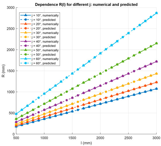
Figure 4.
Comparison of data obtained numerically and using the dependence derived by symbolic regression method.
To derive an analytical dependence of the optimal troughing radius Ropt on belt width l and angle of repose j employed symbolic regression using the PySR library [30]. This approach automatically discovers compact, interpretable mathematical expressions that approximate the data without prescribing the functional form a priori [31,32].
As input, we used a dataset comprising over one thousand l, j combinations with their corresponding Ropt, obtained via numerical optimization of the bulk cross-sectional area.
Data processing involved preliminary cleaning, normalization of column names, type casting, and splitting the dataset into training (80%) and test (20%) subsets [33]. Model training employed a set of basic operators—addition, subtraction, multiplication, division, and exponentiation—together with unary functions (square root, logarithm, exponential, and reciprocal) [34]. The algorithm was configured to search for expressions that balance accuracy and parsimony, enforcing a complexity cap and a parsimony penalty to discourage overly complex formulas and overfitting [35].
As a result, the algorithm yielded a relation that best captures the system’s behavior while satisfying the expected monotonicity criteria. The optimal troughing radius is accurately described by:
The derived analytical dependence is based on a geometric analysis of the circular segment and the triangle formed by the belt chord and the radius of curvature, and it approximates the numerical solutions of the underlying transcendental equation for the maximum cross-sectional area. Figure 4 presents a comparison between the numerical values of and the results obtained from this analytical relation, while Table 2 shows representative examples of the agreement between the numerical and predicted values for various combinations of belt width and angle of repose .
Table 2.
Comparison of Numerical and Predicted Ropt.
For a quantitative assessment of the approximation accuracy, standard metrics were computed using the same computed values of that were employed for training the PySR model, namely the root-mean-square error:
the mean absolute error:
and the coefficient of determination:
where are the numerical values of , are the values computed from the derived formula, and is the sample mean. For the obtained relation, the metrics are , , and . These indicators confirm the suitability of the formula for engineering calculations.
Verification of physical plausibility showed that the model correctly reproduces the expected trends: for a fixed angle , the optimal radius increases monotonically with increasing belt width , whereas for a fixed , the value of decreases as the angle of repose increases. This is consistent with the expected behaviour of the system: at larger angles of repose the heap becomes steeper and lower in height; so, a smaller trough radius is sufficient to contain the bulk material.
A universal formula has been derived for computing the maximum cross-sectional area of the bulk load on the belt.
recognizing that AB denotes the suspension spacing, we derived the spacing at which the belt’s bulk cross-sectional area attains its maximum:
We then determine the optimal suspension spacing, ABopt and compare it with the numerically obtained spacing (Figure 5) for belt widths l ranging from 1000 to 3000 (mm) in 250 (mm) increments, at an angle of repose j = 30°.
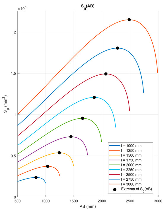
Figure 5.
Dependence of the cross-sectional area on the distance between supports AB.
From Equation (17), for l = 2000 (mm) and j = 30° ABopt = 1.6396 (m), A direct numerical search shows that Sg attains its maximum at AB = 1.6540 (m). The relative difference of 0.87% indicates close agreement and corroborates the validity of Equation (18) for engineering use.
3.2. Determination of the Payload Mass per Unit Length
Having determined the maximum cross-sectional area of the bulk on the belt, Sg = max the next step is to compute the mass of the conveyed material per unit belt length (per meter). The characteristics of the bulk cargo are presented in Table 3.
Table 3.
Bulk Material Properties.
Over a 1 m belt segment, the bulk volume is numerically equal to the cross-sectional area, Sg (m3/m); so, the payload mass per unit length is obtained by [36]. When sizing the magnetic suspension, [37] we employ to obtain a conservative (upper-bound) [38] estimate of the payload mass per meter.
3.3. Accounting for the Belt Mass
In addition to the payload, the belt’s self-weight contributes to the mass per unit length of the conveyor [39]. Accurate determination of the total mass per unit length therefore requires explicit inclusion of the belt mass.
The belt mass per unit length mbelt (kg/m) depends on its construction—most notably the carcass (reinforcement) type and the thickness of the rubber covers. The two principal belt families—textile (fabric-reinforced) and steel-cord—differ markedly in weight: textile belts generally have a lower specific mass, whereas high-strength steel-cord belts are heavier.
For textile (fabric-reinforced) belts handbook data typically report the belt mass per unit length mbelt as an areal mass (areal density) in units of (kg/m2) (see Table 4). To obtain mbelt in (kg/m), multiply the areal mass by the belt width l (in meters).
Table 4.
Areal mass of textile (fabric-reinforced) belts (kg/m2) as a function of fabric type and ply count [40].
3.4. Practical Application and Worked Example
In the preceding sections, a closed-form expression for the maximum bulk cross-sectional area for configuration b (Equation (17)) was obtained. Substituting this function into the general relation between cross-sectional area and mass per unit length (Equation (1)) yields Equation (19), which defines the maximum attainable mass per unit length of the loaded suspended belt:
As shown in Section 2.3, the approximation used to construct Equation (19) reproduces the underlying numerical model with a typical relative error of less than 0.1%; so, the values of computed from Equation (19) inherit this level of accuracy.
As a detailed example, consider a conveyor with a textile (fabric-reinforced) belt TK-300 (four plies, with 4.5/3.5 mm covers) transporting run-of-mine coal. TK-300 is a widely used standard belt type in mining belt conveyors; so, this example highlights that the proposed methodology can be directly applied to conventional off-the-shelf belts when designing suspended, including magnetically levitated, conveyor systems. Let the belt width be , the bulk density , the angle of repose , the operational factor , and the linear mass of the empty belt
The maximum attainable mass per unit length in this example is about . This value can be used directly as the design load for determining the required specific lifting force of the magnetic suspension.
To illustrate the behavior of Equation (19) over a wider range of parameters, additional calculations of were carried out for various combinations of belt width , bulk density , and angle of repose . In all the examples below, the same operational factor and linear mass of the empty belt are used. The examples are summarised in Table 5.
Table 5.
Examples of maximum linear mass for different combinations of parameters.
The numerical values in Table 5 were obtained by substituting the corresponding parameters into Equation (19). The table clearly demonstrates the expected trends: increases with increasing belt width and bulk material density, and it also depends significantly on the angle of repose. These dependencies must be taken into account when specifying the required lifting capacity of the magnetic suspension system.
4. Discussion
This work proposes a reproducible methodology for determining the maximum attainable mass per unit length of a suspended conveyor belt with magnetic levitation. The methodology combines an analytical description of the cross-section for the key geometric configurations (a–d) and its optimization with respect to the troughing radius R and the derivation of an interpretable closed-form law for Ropt(l,j) via symbolic regression. We show that the maximum cross-sectional area is achieved under configuration b, which follows from more complete utilization of the belt width l subject to the geometric constraints on AB and R. Configurations c and d yield the same maximum in the boundary case H = 0, whereas configuration a underperforms due to the absence of troughing.
The resulting compact law is:
It faithfully reflects the underlying physics: at fixed j the optimal radius increases monotonically with belt width l, at fixed l decreases as the angle of repose j. grows. This accords with intuition: a wider belt requires a gentler curvature to retain the pile, whereas a larger angle of repose (steeper flanks) permits a less pronounced trough. Comparison with the numerical solution demonstrates high approximation accuracy, and the monotonicity checks confirm the physical soundness of the result across the entire training domain. An important corollary follows from substituting Ropt(l,j), yields a closed-form expression for the optimal suspension spacing that links trough geometry to the suspension layout.
The practical significance of these results is that maximizing the cross-sectional area Sg,max at a given belt width l and angle j yields a direct increase in throughput without enlarging the conveyor envelope. Combining Ropt(l,j) with the area model Sg(R) and accounting for the fill factor k and bulk density ρ, the total mass per unit length is:
which, in turn, determines the required specific lifting force of the magnetic system. A representative example for a TK-300 textile belt transporting run-of-mine coal yields a total mass per unit length of approximately 1354,3 kg/m and a corresponding specific lifting force of about 13,28 kN/m, establishing realistic requirements for the magnetic suspension and an adequate margin for levitation stability. At the operational level, this translates into reduced wear, lower friction, and improved overall reliability of the conveying line.
This study has recognized limitations. First, the angle of repose j is treated as deterministic and constant, whereas in practice it depends on moisture content, particle-size distribution, particle shape and interparticle cohesion, and under belt motion may differ from the static value (i.e., a dynamic angle). Second, the fill factor k is modeled in aggregate; its dependence on loading regime, vibration, belt speed, and the geometry of the loading device can lead to deviations from the assumed values. Third, the calculations neglect the belt’s bending and transverse stiffness, local edge deformations, and potential loss of slope stability under impact loading.
The foregoing simplifications were adopted deliberately to obtain an upper bound on the mass per unit length, appropriate for the preliminary design stage of the magnetic suspension. Under the stated assumptions—a deterministic, stationary angle of repose j, a high (aggregate) fill factor k, an idealized trough geometry without sagging or local edge deformation; and quasi-static operation without impact disturbances—the quantity ml attains its maximum, i.e., the worst-case for the suspension in terms of the required specific lifting force. This conservative stance ensures that adequate margins in lifting force and levitation stability are specified when selecting the parameters of the magnetic system.
In this study, a quasi-static geometrical–analytical formulation is considered, which makes it possible to obtain an upper estimate of the maximum admissible linear mass of a suspended belt for given material parameters and belt width. Dynamic effects, as well as electromagnetic processes in the suspension system, are deliberately not modelled here: the analytical framework presented is intended as an initial stage that defines the limiting static level of loading. In subsequent work, it will serve as the basis for magnetic modelling tasks and for dedicated laboratory experiments aimed at verifying and refining the limiting linear mass of the suspended belt under realistic operating conditions.
The proposed methodology provides a principled means of selecting the trough geometry and suspension parameters for magnetically levitated conveyors. The combination of analytical geometry with symbolic regression yields compact formulas that deliver high accuracy across a wide range of operating conditions and are readily integrated into standard engineering design and verification procedures.
5. Conclusions
This study presents a reproducible approach to determining the maximum linear mass of a magnetically suspended conveyor belt, combining an analytic description of the cross-sectional geometry for configurations a–d, optimization with respect to the troughing radius R, and symbolic regression (PySR) to obtain a compact, interpretable law . The dataset was formed from the numerical solution of the cross-sectional area maximization problem. In PySR, we used a physically meaningful set of operations and arbitrary exponents, limited the depth of expression trees, and selected models using error–complexity penalties; candidate formulas were further filtered by a priori physical criteria (monotonicity (, , correct limiting behavior), with a train/validation split to control overfitting. The resulting exhibits the expected monotonicity (increasing with l, decreasing with j), agrees well with numerical calculations, and provides a closed-form link to the suspension spacing ;); the maximum cross-sectional area is achieved in configuration B because it makes the fullest use of the belt width under the geometric constraints on AB and R; in the boundary case H = 0, configuration c reduces to d, whereas a predictably underperforms due to the absence of troughing. Incorporating into the computational loop together with the area model and belt/material parameters yields design-ready equations for the maximum linear mass and the required lifting force per unit length.
Author Contributions
Conceptualization, S.A.G.; Methodology, A.N.E.; Software, J.W.; Formal analysis, A.Y.Z. All authors have read and agreed to the published version of the manuscript.
Funding
This research was carried out with financial support under the state assignment of the Ministry of Science and Higher Education of the Russian Federation (No. 075-03-2024-082-2).
Data Availability Statement
Additional information, in particular the training code and the database for model development, is available at https://github.com/sgordin990-create/DETERMINING-THE-MAXIMUM-LINEAR-MASS-OF-A-CONVEYOR-BELT-BASED-ON-PYSR-SYMBOLIC-REGRESSION (accessed on 23 September 2025).
Acknowledgments
The authors gratefully acknowledge the Department of Mining Machines and Complexes of T. F. Gorbachev Kuzbass State Technical University for their support and constructive discussions that contributed to this research.
Conflicts of Interest
The authors declare no conflicts of interest. The funders had no role in the design of this study; in the collection, analyses, or interpretation of data; in the writing of the manuscript; or in the decision to publish the results.
Abbreviation
The following abbreviation is used in this manuscript:
| PySR | Python Symbolic Regression (SymbolicRegression.jl) |
References
- Deka, R.; Borthakur, P.P.; Baruah, E.; Sarmah, P.; Saikia, M. A comprehensive review on mechanical conveyor systems: Evolution, types, and applications. Int. J. Nat. Eng. Sci. 2024, 18, 164–183. [Google Scholar]
- Galkin, V.I.; Sheshko, E.E. Belt conveyors at the current stage of development in mining machinery. Gorn. Zhurnal 2017, 9, 85–90. (In Russian) [Google Scholar] [CrossRef][Green Version]
- Perten, Y.A. Konveyernyi transport XXI veka. Transp. Ross. Federatsii. Zhurnal O Nauk. Prakt. Ekon. 2005, 1, 42–43. (In Russian) [Google Scholar]
- Hu, K.; Jiang, H.; Zhu, Q.; Qian, W.; Yang, J. Magnetic Levitation Belt Conveyor Control System Based on Multi-Sensor Fusion. Appl. Sci. 2023, 13, 7513. [Google Scholar] [CrossRef]
- Wang, S.; Hu, K.; Li, D. Analysis and experimental research on air gap characteristics of permanent magnet low-resistance belt conveyor. IET Sci. Meas. Technol. 2018, 12, 963–971. [Google Scholar] [CrossRef]
- Cheng, G.; Guo, Y.C.; Hu, K.; Wang, P.Y. Magnetic Belt Conveyor Running Stability Analysis. Appl. Mech. Mater. 2013, 437, 682–685. [Google Scholar] [CrossRef]
- Zakharov, A.Y.; Erofeeva, N.V. Vozmozhnosti snizheniya dinamicheskikh nagruzok na konveyernuyu lentu. Gorn. Oborud. I Elektromekhanika 2018, 6, 3–14. (In Russian) [Google Scholar] [CrossRef]
- Vasil’ev, K.A.; Nikolaev, A.K. Lentochnyi konveyer s podvesnoy lentoy na khodovykh oporakh skolzheniya. J. Min. Inst. 2008, 178, 35–39. (In Russian) [Google Scholar]
- Tang, X.; Hashimoto, S.; Kurita, N.; Kawaguchi, T.; Ogiwara, E.; Hishinuma, N.; Egura, K. Development of a Conveyor Cart with Magnetic Levitation Mechanism Based on Multi Control Strategies. Appl. Sci. 2023, 13, 10846. [Google Scholar] [CrossRef]
- Robinson, P.W.; Orozovic, O.; Meylan, M.H.; Wheeler, C.A.; Ausling, D. Optimization of the cross section of a novel rail running conveyor system. Eng. Optim. 2022, 54, 1544–1562. [Google Scholar] [CrossRef]
- Ordin, A.A.; Nikol’sky, A.M.; Grishchenko, M.A. Optimizing Cross-Section Outline of Bulkload on Belt Conveyor. J. Min. Sci. 2024, 60, 117–123. [Google Scholar] [CrossRef]
- Kuleshov, V.G. Opredelenie radiusa krivizny izgibayushchegosya lentochnogo konveyera s povorotnym ustroystvom. Gorn. Informatsionno-Anal. Byulleten’ 2006, 5, 5. (In Russian) [Google Scholar]
- Wang, S.; Li, D.; Guo, Y. Research on Magnetic Model of Low Resistance Permanent Magnet Pipe Belt Conveyor. 3D Res. 2016, 7, 23. [Google Scholar] [CrossRef]
- Wang, Z.; Hu, K.; Guo, Y.; Wang, S. Optimization on detent force characteristics of the permanent magnet suspension belt conveyor. Adv. Mech. Eng. 2018, 10, 1–13. [Google Scholar] [CrossRef]
- Tolkachev, E.N. Vliyanie nekotorykh konstruktivnykh i rezhimnykh parametrov konveyera s podvesnoy lentoy i raspredelennym privodom na ego tekhnicheskie kharakteristiki. Nauchno-Tekhnicheskii Vestn. Bryanskogo Gos. Univ. 2017, 1, 67–80. (In Russian) [Google Scholar] [CrossRef]
- Babyr’, A.Y.; Babyr’, N.V. Analiz sovremennykh sredstv tsifrovizatsii v logistike. In Sbornik Trudov; Federal’noe gosudarstvennoe avtonomnoe obrazovatel’noe uchrezhdenie vysshego obrazovaniya “Sankt-Peterburgskii politekhnicheskii universitet Petra Velikogo”: Saint Petersburg, Moscow, 2019; pp. 138–143. Available online: https://www.elibrary.ru/item.asp?id=42831388 (accessed on 17 October 2025). (In Russian)
- Nguyen, K.L.; Gabov, V.V.; Zadkov, D.A. Improving efficiency of cleanup and coal flow formation on conveyor by shearer loader with accessorial blade. Eurasian Min. 2019, 1, 37–39. [Google Scholar] [CrossRef]
- Nguyen, K.L.; Gabov, V.V.; Zadkov, D.A. Improvement of drum shearer coal loading performance. Eurasian Min. 2018, 2, 22–25. [Google Scholar] [CrossRef]
- Hrabovský, L.; Fries, J. Transport Performance of a Steeply Situated Belt Conveyor. Energies 2021, 14, 7984. [Google Scholar] [CrossRef]
- Masaki, M.S.; Zhang, L.; Xia, X. A Comparative Study on the Cost-effective Belt Conveyors for Bulk Material Handling. Energy Procedia 2017, 142, 2754–2760. [Google Scholar] [CrossRef]
- Ilic, D.; Wheeler, C. Measurement and simulation of the bulk solid load on a conveyor belt during transportation. Powder Technol. 2017, 307, 190–202. [Google Scholar] [CrossRef]
- Zeng, F.; Yan, C.; Wu, Q.; Wang, T. Dynamic Behaviour of a Conveyor Belt Considering Non-Uniform Bulk Material Distribution for Speed Control. Appl. Sci. 2020, 10, 4436. [Google Scholar] [CrossRef]
- Hrabovský, L. Cross-sectional area of the belt conveyor with a three-idler set. Perners Contacts 2011, 6, 62–67. [Google Scholar]
- Perten, Y.; Pelenko, I.; Erina, E. Ustoichivost’ peremeshcheniya nasypnogo gruza v krutonaklonnykh vertikal’nykh trubchatykh konveyerakh. Nauchnyi Zhurnal NIU ITMO. Seriya Protsessy I Apparaty Pishchevykh Proizv. 2006, 1, 37–42. (In Russian) [Google Scholar]
- Stepanovich, P.O. Opredelenie geometricheskikh parametrov zheloba podvesnoy konveyernoy lenty. Gorn. Informatsionno-Anal. Byulleten 2007, 6, 6. (In Russian) [Google Scholar]
- Gordin, S. Determining-the-Maximum-Linear-Mass-of-a-Conveyor-Belt-Based-on-PySR-Symbolic-Regression. Python Code, 23 September 2025. Available online: https://github.com/sgordin990-create/DETERMINING-THE-MAXIMUM-LINEAR-MASS-OF-A-CONVEYOR-BELT-BASED-ON-PYSR-SYMBOLIC-REGRESSION (accessed on 23 September 2025).
- Tsakalakis, K.; Michalakopoulos, T. Mathematical modeling of the conveyor belt capacity. In Proceedings of the 8th International Conference for Conveying and Handling of Particulate Solids (CHoPS), Tel-Aviv, Israel, 3–7 May 2015. [Google Scholar]
- Sutisna, N.A.; Sudarso, L. Calculation of Belt Conveyor for Transferring Steel Grit in Sandblasting Room. J. Rekayasa Mesin 2021, 12, 521–531. [Google Scholar] [CrossRef]
- Munir, H.A.; Zakaria, A.; Ponniran, A.; Rahman, M.T.A.; Marimuthu, T. Investigation of The Dynamic Deflection of Conveyor Belts Via Simulation Modelling Methods on Idler Factor. J. Phys. Conf. Ser. 2022, 2312, 012027. [Google Scholar] [CrossRef]
- Cranmer, M.; Sanchez-Gonzalez, A.; Battaglia, P.; Xu, R.; Cranmer, K.; Spergel, D.; Ho, S. Discovering Symbolic Models from Deep Learning with Inductive Biases. arXiv 2020, arXiv:2006.11287. [Google Scholar] [CrossRef]
- Cranmer, M. Interpretable Machine Learning for Science with PySR and SymbolicRegression.jl. arXiv 2023, arXiv:2305.01582. [Google Scholar] [CrossRef]
- Sorour, S.S.; Saleh, C.A.; Shazly, M. Integrating machine learning and symbolic regression for predicting damage initiation in hybrid FRP bolted connections. Sci. Rep. 2025, 15, 18564. [Google Scholar] [CrossRef] [PubMed]
- Tonda, A. Review of PySR: High-performance symbolic regression in Python and Julia. Genet. Program. Evolvable Mach. 2024, 26, 7. [Google Scholar] [CrossRef]
- Cranmer, M.D. Interpretable Machine Learning for the Physical Sciences. Ph.D. Thesis, Princeton University, Princeton, NJ, USA, 2023. Available online: https://dataspace.princeton.edu/handle/88435/dsp01sn00b201q (accessed on 1 September 2025).
- Schmidt, M.; Lipson, H. Distilling Free-Form Natural Laws from Experimental Data. Science 2009, 324, 81–85. [Google Scholar] [CrossRef] [PubMed]
- Jeftenić, B.; Ristić, L.; Bebić, M.; Štatkić, S.; Mihailović, I.; Jevtić, D. Optimal utilization of the bulk material transportation system based on speed controlled drives. In Proceedings of the XIX International Conference on Electrical Machines (ICEM 2010), Rome, Italy, 6–8 September 2010; pp. 1–6. [Google Scholar] [CrossRef]
- Bortnowski, P.; Król, R.; Ozdoba, M. Modelling of transverse vibration of conveyor belt in aspect of the trough angle. Sci. Rep. 2023, 13, 19897. [Google Scholar] [CrossRef] [PubMed]
- Beakawi Al-Hashemi, H.M.; Baghabra Al-Amoudi, O.S. A review on the angle of repose of granular materials. Powder Technol. 2018, 330, 397–417. [Google Scholar] [CrossRef]
- Webb, C.; Sikorska, J.; Khan, R.N.; Hodkiewicz, M. Developing and evaluating predictive conveyor belt wear models. Data-Centric Eng. 2020, 1, e3. [Google Scholar] [CrossRef]
- BashRezina. Ves, Massa Konveyernoy Lenty, Kvadratnyi Metr v kg, BashRezina, ves Transporternoy Lenty. Available online: https://www.rezina.info/articlesid103.html (accessed on 29 August 2025). (In Russian).


Disclaimer/Publisher’s Note: The statements, opinions and data contained in all publications are solely those of the individual author(s) and contributor(s) and not of MDPI and/or the editor(s). MDPI and/or the editor(s) disclaim responsibility for any injury to people or property resulting from any ideas, methods, instructions or products referred to in the content. |
© 2025 by the authors. Licensee MDPI, Basel, Switzerland. This article is an open access article distributed under the terms and conditions of the Creative Commons Attribution (CC BY) license (https://creativecommons.org/licenses/by/4.0/).