GEOSAT 2 Atmospherically Corrected Images: Algorithm Validation ^†

Abstract

Solar radiation reflected by the Earth’s surface to satellite sensors is modified by its interaction with the atmosphere. The application of atmospheric correction of optical satellite imagery is an essential and needed pre-processing tool for modeling biophysical variables, multi-temporal analysis, and digital classification processes. As a result, true surface reflectance values are obtained without atmosphere influence. To assess this process, GEOSAT (part of the ESA’s Third-Party Mission Programme) performs an optimization of the GEOSAT 2 very high resolution (VHR) multispectral imagery adapting the well-known 6S model to the different wavelengths covered by the GEOSAT 2 spectral bands (VHR, PAN). The 6S model predicts surface reflectance (BOA) using information from the apparent reflectance (TOA) captured by the satellite sensor and the corresponding atmospheric conditions. To perform the atmospheric correction (AC), both the configuration of the atmosphere at the time of capture and the conditions of scene pointing and luminosity, must be considered. The first is mainly determined by three values: water vapor, ozone, and the number of air-suspended particles (aerosols). For the latter, the geometry of the scene, as well as the respective sun and sensor observation positions are the values to be considered. To validate the resultant GEOSAT 2 AC images, obtained from applying the GEOSAT atmospheric correction algorithm, different common areas between these and Sentinel-2 L2A products have been selected. Then, band-by-band (R, G, B, and NIR) operations were performed, such as the calculation of the mean square error (RMSE) and a regression analysis. Then, spectral profiles for the three generic land coverages (vegetation, soil, and water) were also gathered over the spectral range of GEOSAT 2 and S2 corresponding bands. The outcomes, once analyzed, lead us to conclude that the results obtained by applying the promising GEOSAT AC algorithm are satisfactory and seem to correctly estimate BOA reflectance values for vegetation and water coverages. To extend the study and improve the result, ground reflectance values will be required.

1. Introduction

Radiation leaving the Earth’s surface experiences an important interaction with the atmosphere before it is registered by a satellite sensor. There are many ways to compensate for atmospheric contributions to an Earth image observed by an optical satellite sensor. They vary from empirical methods, which modify the brightness of each sensor spectral band, to more robust procedures based on complex and robust physical models describing the atmospheric radiation paths and considering the most contributing atmospheric gases and aerosols. Within the latter, Radiative Transfer models are the most appropriate methods, as they are able to effectively couple and compensate the mentioned atmospheric effects. For several decades, efforts have been made to implement computer codes that simulate and correct for atmospheric disturbances on optical observations. This is the case for the MODTRAN (MODerate resolution atmospheric TRANsmission) [1]. Several computer packages have been implemented based on the MODTRAN philosophy, such as the 6S (Second Simulation of a Satellite Signal in the Solar Spectrum) [2], which focusses on correcting for atmospheric effects on airborne and satellite optical images. An important feature of the 6S code is that it can be optimized and customized for specific Earth observing systems, which is the case for GEOSAT 2 imagery. In addition to the already demonstrated good performance of these sophisticated atmospheric correction packages, their application to a particular study and imagery must always be validated in order to assess the uncertainty of the correction process. This study presents results of the optimization of the 6S code for producing GEOSAT 2 level 2 (DE2) products and the respective evaluation of the corrected imagery. For this purpose, processed GEOSAT 2 DE2 and SENTINEL 2A MSIL2A products with close overpasses have been used to preliminary assess the suitability of the GEOSAT 2 atmospheric correction processor.

2. Model Description

The GEOSAT 2 Surface Reflectance (SR) product is derived from the standard radiance product being processed first to TOA reflectance and then atmospherically corrected to BOA reflectance using the well-known radiative transfer (RT) method 6S [2,3,4]. This algorithm has been configured and applied to the different wavelengths covered by the GEOSAT 2 spectral bands (VHR, PAN). For the sake of simplicity and speed we have considered only the bidirectional reflectance (BDR), considering a uniform, or Lambertian, surface. Based on the radiative transfer theory and assuming that the target is a Lambertian surface, the surface reflectance ($\rho$), in terms of the at-sensor radiance ($L$), can be expressed as follows:

$$\rho =\pi \left(L-L_p\right)/\tau \left(E_{dir}+E_{dif}\right)$$

(1)

The following additional parameters of this function are all obtained by executing the 6S model: the path radiance ($L_p$), the transmissivity ($\tau$) from surface to satellite, taking into account the transmissivities, caused by both absorption and scattering, the direct solar irradiance ($E_{dir}$), and the diffuse solar irradiance ($E_{dif}$).

A typical orthorectified GEOSAT 2 image can have more than 30 million pixels. Thus, considering a pixel-wise 6S model execution results in excessive time demand. To reduce the time needed to retrieve BOA reflectance products, an optimization approach, based on lookup tables (LUT), has been performed on GEOSAT 2 imagery. Thus, the ${\mathrm{O}}_3 \mathrm{and} {\mathrm{H}}_2\mathrm{O}$ values are derived from the spatial–temporal table defined in [5] which provides us a valid approximation. On the other hand, MERRA-2 service from the Global Modeling and Assimilation Office (of the National Aeronautics and Space Administration—NASA), is used to retrieve closer AOT values to GEOSAT 2 image sensing time. Concretely, the hourly (M2T1NXAE [6]) and monthly (M2TMNXAER [7]) aerosol optical thickness at 550 nm are accessed from this NASA service, moreover acquisition geometry angles are taken to center time, and surface elevation is determined through the SRTM 1 Arc-Second Global (Earth Resources Observation and Science (EROS) Center (USGS), 2018) (30 m) elevation data from USGS/NASA [8].

3. Model Validation

To assess the atmospheric correction method for GEOSAT 2 (DE2) products, we utilized atmospherically corrected Sentinel 2 (S2) mission level 2A products. The evaluation procedure involved selecting a common area between both products and resample DE2 products to coincide with the S2 MSI spectral bands resolution. The bands and their spectral ranges are as follows:

For Sentinel 2, there are slight differences in the spectral sensitivity of the MSI instruments aboard the S2A and S2B missions., but the spectral response sensitivity functions can be considered practically identical between both missions for the bands considered in this study. Regarding the spectral sensitivity for the DE2 mission bands, no data are available for this study. However, according to the below table (Table 1), the central bands of the DE2 mission are nearly coincident with those of S2, as well as their spectral widths. In this context, for the forthcoming comparison, it is assumed that analogous spectral bands are being evaluated between DE2 and S2.

Table 1. Spectral resolution DE2 vs. S2.

Number of DE2 Band	DE2λ_central, [λ] (µm)	Number of S2 Band	S2λ_central, [λ] (µm)
1 (blue)	0.496 − [0.466; 0.525]	B2 (blue)	0.490 − [0.458; 0.523]
2 (green)	0.566 − [0.532; 0.599]	B3 (green)	0.560 − [0.543; 0.578]
3 (red)	0.667 − [0.640; 0.697]	B4 (red)	0.665 − [0.650; 0.680]
4 (NIR)	0.831 − [0.770; 0.892]	B8 (NIR)	0.842 − [0.785; 0.900]

For the validation of the algorithm, several procedures have been considered:

• First, the root mean square error (RMSE_bi) has been found, band by band, between the values of the product DE2 and S2.
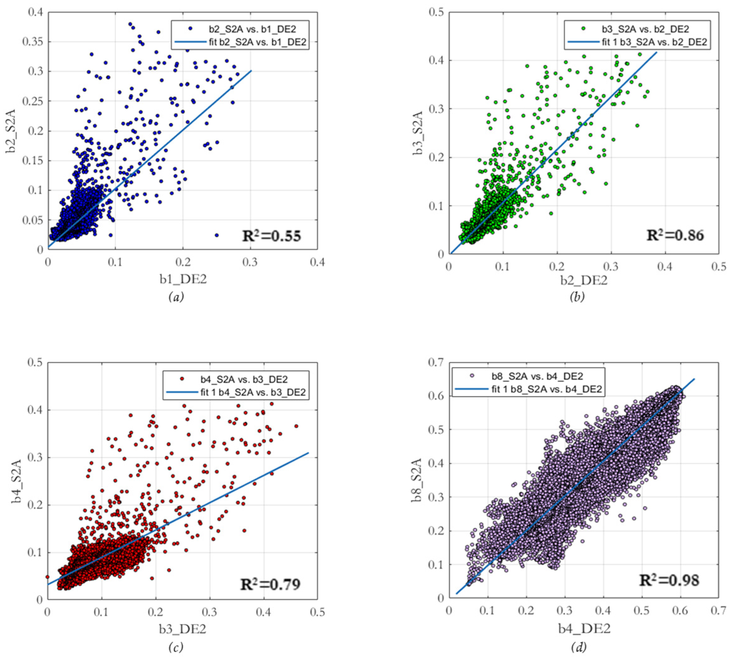
• The second procedure relied on a regression analysis between the corresponding bands of both products, fitting a linear function to the two datasets. In this analysis, the regression coefficient (R²) and the fitting error (RMSE) are obtained, where the latter can be interpreted as a deviation from the fitted function.
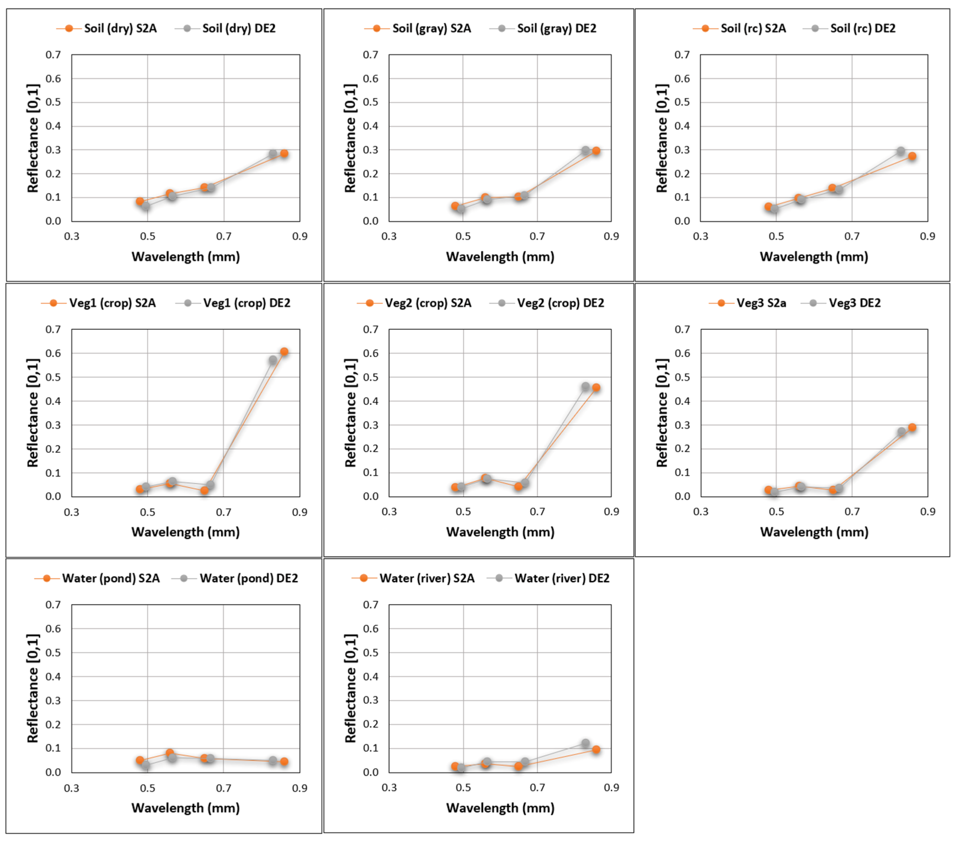
• Thirdly, for generic land cover types such as vegetation, soil, and water, spectral profiles are acquired at specific positions within the study area, and these profiles are depicted graphically.

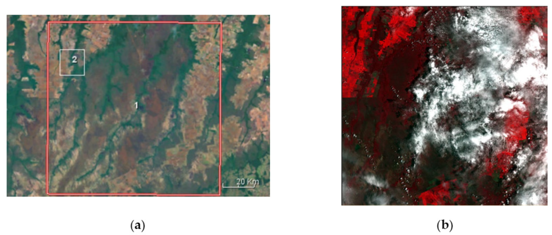
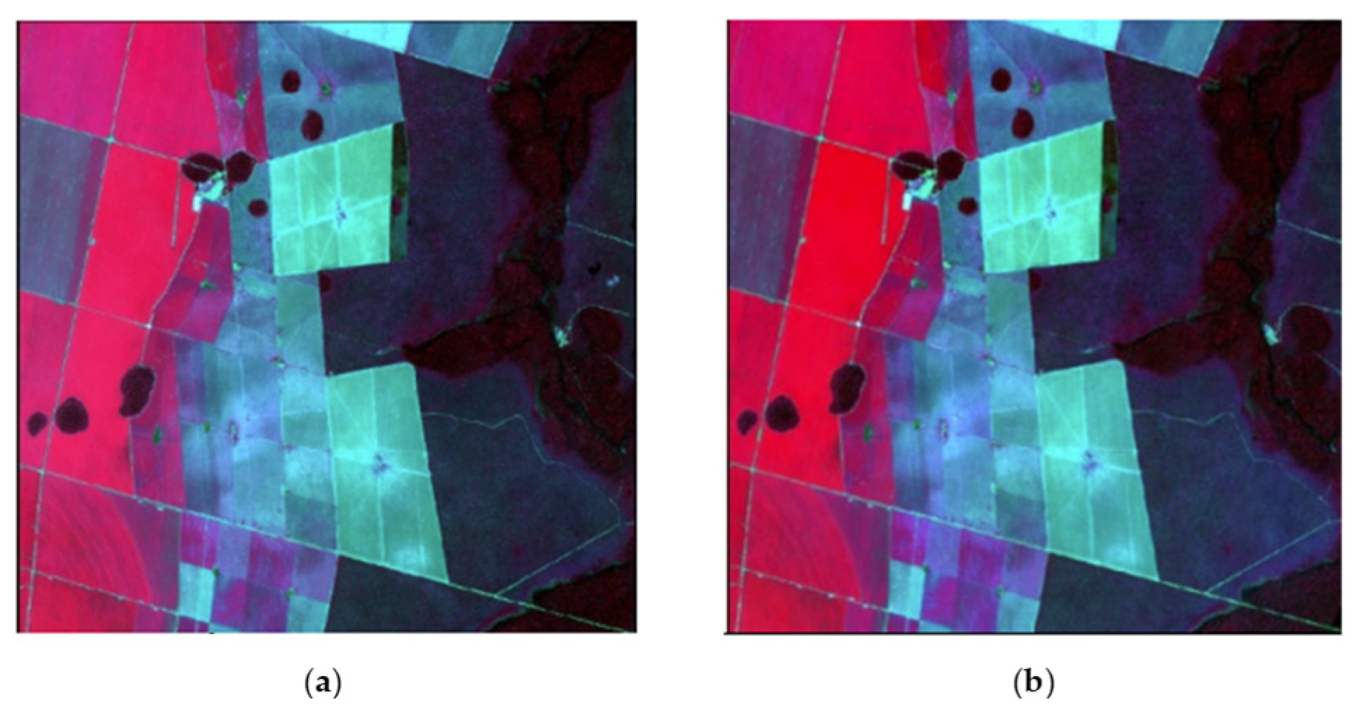
Overall Validation: Brazil

Figure 1 displays the location of the DE2 product, acquired on 25 November 2021 (20211125), in relation to the S2A product acquired on the same day (Table 2). The elapsed time between the two is approximately 39 min.

Figure 1. (a) Relative position between the products DE2 and S2A; (b) S2A product.

Table 2. Product Id for DE2 and S2A.

Product Id	Acquisition Date
DE2_MS4_L1C_000000_20211125T144952_20211125T144954_DE2_40296_88C0	20211125, 14:49:54
S2A_MSIL2A_20211125T141051_N0301_R110_T21LUE_20211125T164741	20211125, 14:10:51

The relative location between DE2 and S2A products is depicted in Figure 1a, in white and red, respectively; whereas Figure 1b illustrates the area observed by the S2A product and the atmospheric conditions at the time of observation for both products.

According to the provided information, DE2 product data have been acquired with an almost nadiral geometry (roll = 3, pitch = 0). Nevertheless, it is noted that for the S2 missions, the angle of observation or incidence over the scene can vary between 2 degrees and 12 degrees, depending on the observed zone, being the average angle in this zone between 2.6° and 8.5°. DE2 and S2A products were acquired with similar viewing geometries. It is worth noting that the common observed area in both images lies within the lowest incidence angles.

After cropping out the common areas between both products, two images are obtained with the same number of rows and columns. The resulting images are shown in Figure 2. It should be noted that the product DE2 was resampled to the spatial resolution (10 m) corresponding to the (VIS-NIR) bands of the MSI instrument.

Figure 2. Spatial scope for atmospheric correction validation; upper left corner, X_ul = 309,275 m and Y_ul = 8,479,905 m; lower right corner, X_lr = 316,135 m and Y_lr = 8,473,115; spatial resolution 10 m, proj/ref.sist.geod. (TM 21, WGS 84) (a) DE2 (b4-R, b3-G, b2-B); (b) S2A (b8-R, b4-V, b3-A).

It was not possible to select a larger area due to the atmospheric conditions that affect both products. For this area, the RMSE_bi values obtained are shown in the table below:

In general, it can be observed that the spectral differences are very low for the first three bands. Although the greatest differences are observed between bands B4_DE2 and B8_S2B, they remain relatively low. In spectral terms, these differences can be considered suitable for all bands in the two images.

In the second procedure, based on a regression analysis between the bands indicated in Table 3, the regression coefficients (R²) and the deviations or RMSE_aj values of the fit, as shown in Table 4, were obtained. Subsequently, Figure 3 displays the graphs of these regressions.

Table 3. Mean squared errors between DE2/S2B bands.

DE2 Bands	S2B Bands	RMSEbi
B1	B2	0.0106
B2	B3	0.0086
B3	B4	0.0151
B4	B8	0.0325

Table 4. R² and band deviation DE2/S2B.

DE2 Bands	S2B Bands	R2	RMSEaj
B1	B2	0.55	0.0096
B2	B3	0.86	0.0154
B3	B4	0.79	0.0079
B4	B8	0.98	0.0179

Figure 3. Regression analysis (Vertical/Horizontal axis units [0,1] a.u.). (a) Blue bands, Band 2 S2A vs. Band 1 DE2; (b) Green bands, Band 3 S2A vs. Band 2 DE2; (c) Red bands, Band 4 S2A vs. Band 3 DE2; (d) NIR bands, Band 8 S2A vs. Band 4 DE2.

Except for the blue bands (DE2 and S2A), the results obtained from the regression analysis are generally satisfactory. All coefficients are above 0.8 (R² ≥ 0.8), except for the two above-mentioned blue bands. The results from both methods are consistent with each other. Furthermore, according to Table 3, the bands that fit the best are Band 4 of DE2 and Band 8 of S2A (R² = 0.98), which, based on the obtained result, would be practically identical. Given the outcomes observed for Bands 1 and 2 of DE2 and S2A, respectively, it would be advisable to extend the analysis to a new area within the same products.

The third evaluation has been conducted through the measurement and comparison of spectral profiles. Three cases have been selected for vegetation and soil, while for water, only two positions could be identified: the graphical representation shows on the horizontal axis the spectral resolution (λ) in micrometers (µm), and on the vertical axis the reflectance value between 0 and 1. The results are presented in the below Figure 4 and Table 5:

Figure 4. Vegetation, soil and water spectral profiles comparison between DE2/SE2 bands.

Table 5. Vegetation, soil and water spectral profiles comparison between DE2/SE2 bands. Including XY coordinates in UTM 21, WGS84.

DE2/S2A	DE2	S2A	DE2	S2A	DE2	S2A	DE2	S2A
	Soil: Dry (313459, 8479785)		Soil: Gray (313459, 8479785)		Soil: Road Crossing (313459, 8479785)		Veg 1 (Crop) (313459, 8479785)
B1/2	0.062	0.083	0.052	0.062	0.052	0.060	0.042	0.029
B2/3	0.104	0.117	0.090	0.100	0.092	0.097	0.064	0.056
B3/4	0.140	0.141	0.109	0.103	0.134	0.138	0.049	0.024
B4/8	0.285	0.283	0.299	0.294	0.295	0.272	0.572	0.606
DE2/S2A	Veg 2 (crop) (313459, 8479785)		Veg 3 (forest) (313459, 8479785)		Water (pond) (313459, 8479785)		Water (river) (313459, 8479785)
B1/2	0.041	0.037	0.020	0.027	0.029	0.048	0.017	0.024
B2/3	0.073	0.077	0.042	0.043	0.059	0.080	0.043	0.036
B3/4	0.057	0.040	0.036	0.057	0.059	0.058	0.043	0.024
B4/8	0.462	0.456	0.272	0.462	0.049	0.043	0.122	0.092

4. Results

For the selected analysis area, based on the obtained spectral profiles, the following considerations are made. There are no significant differences detected among the various types of land covers, and a good agreement is observed among all profiles, including vegetation, soils, and water. The differences typically range between 1% and 2%, which is quite acceptable for this type of comparison. For these three types of covers and depending on the considered spectral band, these differences are practically imperceptible.

Water appears to maintain a satisfactory spectral behavior. However, due to the scarcity of representative water bodies, only two spectral profiles could be measured. As a result, unlike the results obtained for vegetation and soils, these findings cannot be considered definitive.

5. Conclusions

This study shows the preliminary results obtained using the atmospheric correction processor for GEOSAT 2 products based on the 6S code. Although the spectral resolutions between the GEOSAT 2 and the MSI systems are slightly different, the similarity metrics used provide values that confirm the good performance of this processor. Only the blue bands have a very low R2, which is not revealed by the RMSE between both bands and the differences between the measured spectral values. These results can be considered satisfactory for the chosen area and land cover types. A similar validation has been performed on different geographical areas with different landscapes/landcovers and reaching similar results. In these other cases, the blue bands were highly correlated. This analysis must be expanded with complementary validation methods, such as the use of field measured spectra measured and other statistical quality tests.

References

- Berk, A.; Conforti, P.; Kennett, R.; Perkins, T.; Hawes, F.; van den Bosch, J. MODTRAN6: A major upgrade of the MODTRAN radiative transfer code. In Proceedings of the SPIE 9088, Algorithms and Technologies for Multispectral, Hyperspectral, and Ultraspectral Imagery XX, 90880H, SPIE Defense + Security, Baltimore, MD, USA, 13 June 2014. [Google Scholar] [CrossRef]
- Vermote, E.F.; Tanré, D.; Deuze, J.L.; Herman, M.; Morcette, J.J. Second Simulation of the Satellite Signal in the Solar Spectrum, 6S: An Overview. IEEE Trans. Geosci. Remote Sens. 1997, 35, 675–686. [Google Scholar] [CrossRef]
- Kotchenova, S.Y.; Vermote, E.F.; Matarrese, R.; Klemm, F.J., Jr. Validation of a vector version of the 6S radiative transfer code for atmospheric correction of satellite data. Part I: Path radiance. Appl. Opt. 2006, 45, 6762–6774. [Google Scholar] [CrossRef] [PubMed]
- Second Simulation of a Satellite Signal in the Solar Spectrum–Vector (6SV) User Guide. Available online: https://salsa.umd.edu/files/6S/6S_Manual_Part_1.pdf (accessed on 31 July 2023).
- Atmospheric Corrections with FLAASH. Available online: https://www.l3harrisgeospatial.com/docs/FLAASH.html (accessed on 31 July 2023).
- M2T1NXAER, Global Modeling and Assimilation Office (GMAO) (2015), MERRA-2 tavg1_2d_aer_Nx: 2d,1-Hourly, Time-Averaged, Single-Level, Assimilation, Aerosol Diagnostics V5.12.4, Greenbelt, MD, USA, Goddard Earth Sciences Data and Information Services Center (GES DISC). Available online: https://doi.org/10.5067/KLICLTZ8EM9D (accessed on 31 July 2023).
- M2TMNXAER, Global Modeling and Assimilation Office (GMAO) (2015), MERRA-2 tavgM_2d_aer_Nx: 2d, Monthly Mean, Time-Averaged, Single-Level, Assimilation, Aerosol Diagnostics V5.12.4, Greenbelt, MD, USA, Goddard Earth Sciences Data and Information Services Center (GES DISC). Available online: https://doi.org/10.5067/FH9A0MLJPC7N (accessed on 31 July 2023).
- STRM 1 Arc-Second Global (30 m) Elevation Data. Available online: https://www.usgs.gov/centers/eros/science/usgs-eros-archive-digital-elevation-shuttle-radar-topography-mission-srtm-1 (accessed on 31 July 2023).
Disclaimer/Publisher’s Note: The statements, opinions and data contained in all publications are solely those of the individual author(s) and contributor(s) and not of MDPI and/or the editor(s). MDPI and/or the editor(s) disclaim responsibility for any injury to people or property resulting from any ideas, methods, instructions or products referred to in the content. |
© 2023 by the authors. Licensee MDPI, Basel, Switzerland. This article is an open access article distributed under the terms and conditions of the Creative Commons Attribution (CC BY) license (https://creativecommons.org/licenses/by/4.0/).