Application of the Sliding Window Method to the Short Range Prediction System for the Correction of Precipitation Forecast Errors ^†

Abstract

The SisPI is used in INSMET to provide precipitation forecasts. Generally, these numerical forecasts present errors in precipitation amount as well as position. In order to reduce these errors, in this work, we propose to improve the precision of the precipitation forecast by the implementation of the sliding window method. It is obtained as a result that the spatial error presented by SisPI can be reduced by using a window of size N = 15 and the maximum and average instructions. The quantitative error was decreased more optimally with the medium instruction using the same window size.

1. Introduction

Numerical weather prediction (NWP) has improved substantially in recent decades due to improvements in observational data sets and computing power. Precipitation is one of the key forecast elements within NWP, as a variety of entities such as agriculture, transportation, airlines, etc. require accurate forecasts and are especially interested in as many (spatial, temporal) details as possible [1]. Among the tools available in Cuba for the quantitative forecast of precipitation is the short range prediction system (SisPI) [2]. Although SisPI has a relatively good ability to forecast rainfall, for certain applications it requires an increase in accuracy. For this reason, several efforts are being made by researchers to develop different MOS-type methods that allow achieving lower errors in the forecast of the amount of precipitation and the position of the rainy areas. This research is in this line of work and proposes to improve the precision of the SisPI precipitation forecast by implementing the sliding window method [3].

2. Materials and Methods

2.1. Description of the Study Cases

For the development of this research, eight precipitation events that occurred in different provinces of the country during the year 2020 were used as study cases. Table 1 lists the cases used. It is important to clarify that in this document, due to page number limitations, only the results associated with the rain event that occurred on 1 February 2020, associated with the entry of a cold front, are discussed.

Table 1. Study cases. Severe local storm reports.

No. of Cases	Date	Place, Municipality, and Province
1	1 February 2020	ISCAH and INCA (Institutes of Agricultural Sciences) area on the Tapaste highway, in front of the Tapaste weather station. San José de las Lajas, Mayabeque
2	30 April 2020	Town of Las Mangas, Bankruptcy Hacha. Mayabeque,
3	26 May 2020	San Rafael, Yateras, Guantánamo
4	28 June 2020	El Pavón, in the popular council of Maya Este. Songo-La Maya, Santiago de Cuba
5	2 July 2020	Pinares de Mayarí, Mayarí, Holguín

2.2. Data to Be Used

The SisPI precipitation outputs were used, whose configuration, characteristics, and simulation domains can be consulted in [4]. In particular, the runs with initialization at 00:00 and the one at 12:00 UTC were used and the sliding window method was applied to the 3km resolution domain.

For the verification, the data offered by the satellite precipitation estimation product GPM (Global Precipitation Measurement) was used as the observation [5].

2.3. Sliding Window Method

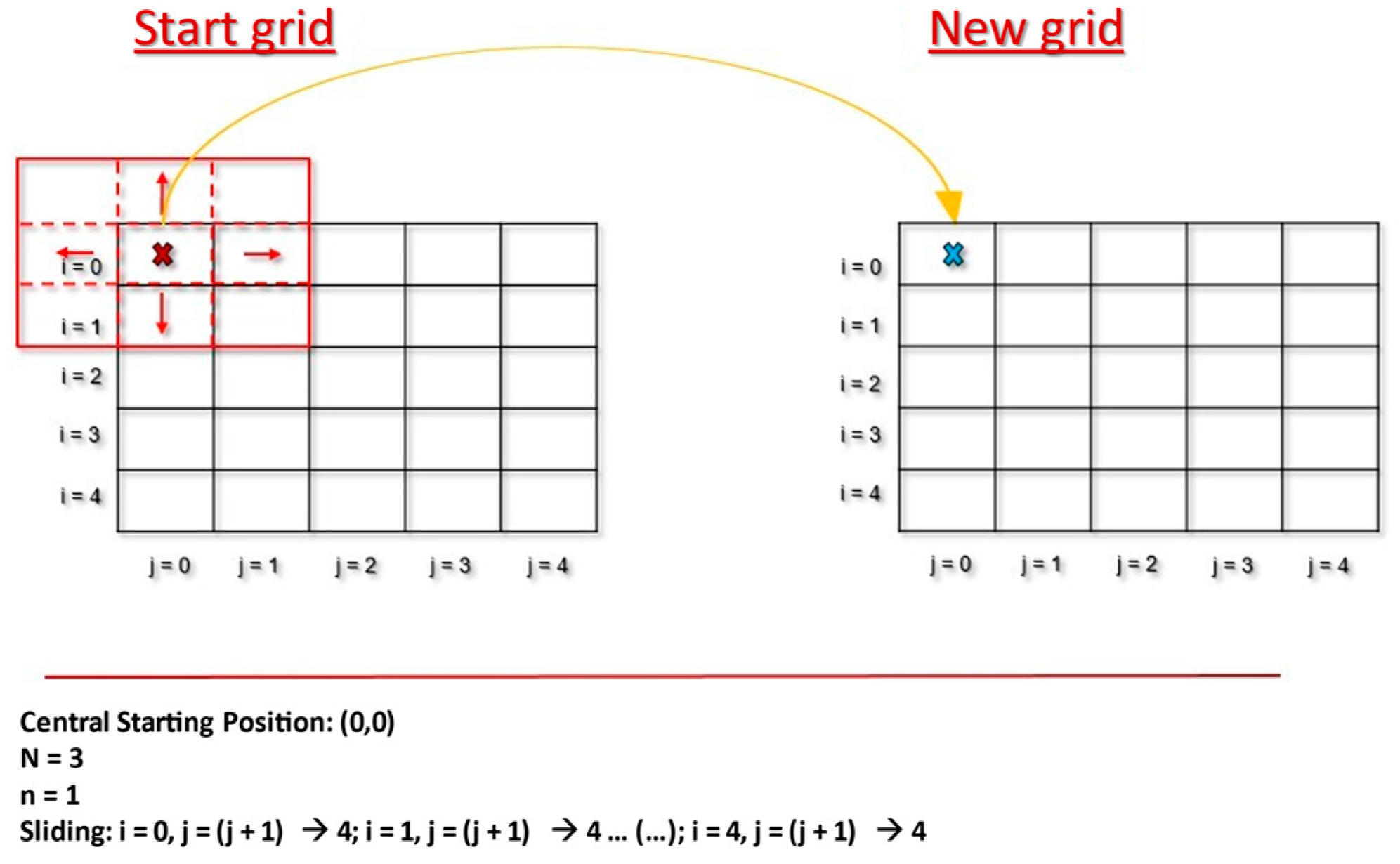
The sliding window technique uses a window of moving space on a grid to select the data for processing. The window moves incrementally forward in space (Figure 1), generating a complete solution each time. In the case of this investigation, each complete solution is exported to a new mesh created with the solutions obtained by this method. Next, with the elements of the window, the mean, the median, and the maximum are calculated. The fundamental parameters of the method are explained below:

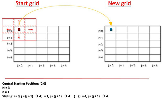
Figure 1. Representation of the sliding window method.

• Position of the window, which is identified according to the position of its center, which, taking into account that the rows will be identified as i, and the columns as j, is given by (i,j);
• Window width or size (N), a total of 7 window sizes were used in this work (N = 3, N = 5, N = 7, N = 9, N = 11, N = 13 and N = 15) in order to select the window width that offers the best results;
• Number of elements of the window width ($n=\frac{N-1}{2}$).

The center of the window will increase so that it will move through each node of the row until it ends, once it reaches the last node of the row. the center will move to the first node of the next row, thus traversing the entire mesh (Figure 1).

2.4. Evaluation

For the evaluation of the window method’s effectiveness, the BIAS and an analysis using the contingency table where CSI, POD, and FAR metrics were calculated were used. The analysis with the latter is not shown in this document.

3. Results

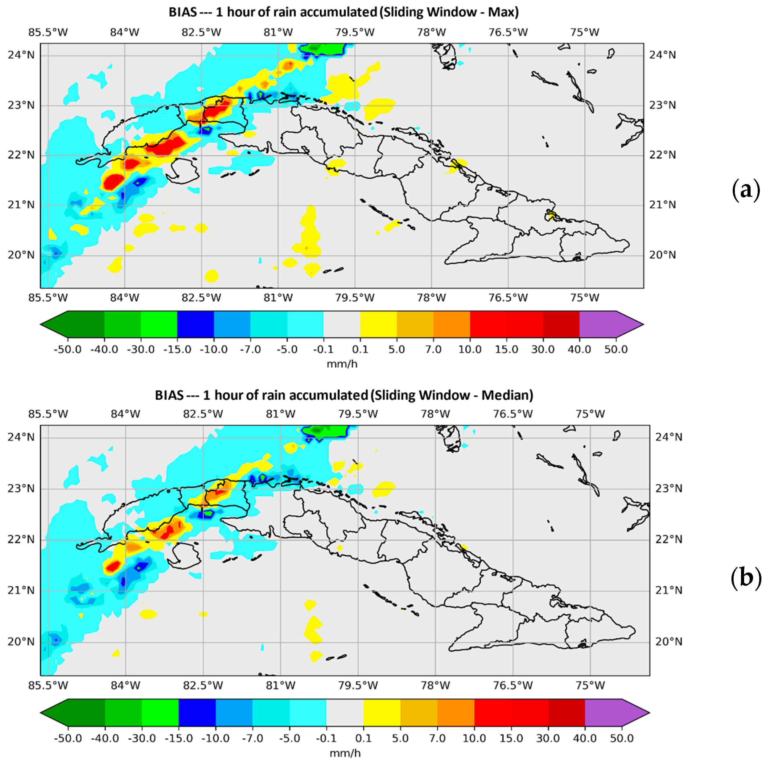
The values obtained when calculating the BIAS for the first case study with the initialization of 12:00 UTC and window sizes N = 3 and N = 15 are analyzed. The objective is to study how well the sliding window method corrected precipitation amount errors. Figure 2 shows that the instructions that improve the output of the SisPI in terms of the amount of forecast precipitation are the mean and the median, with the mean above the median standing out, which achieves more accurate forecasts in this aspect for a window size of N = 15.

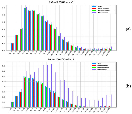
Figure 2. BIAS values of the first case study for the initialization of 12:00 UTC. (a) For window width N = 3. (b) For window width N = 15.

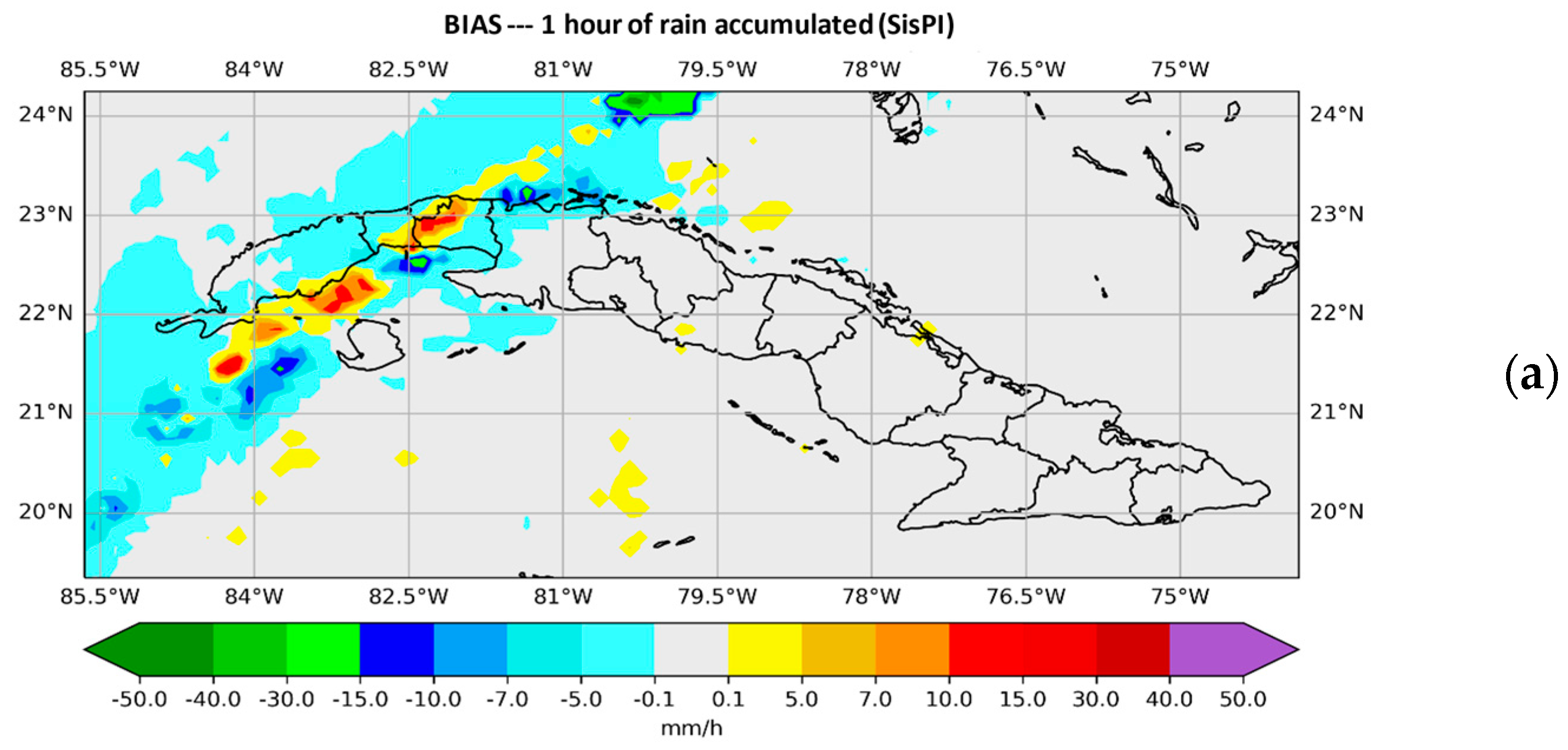
Figure 3 presents the BIAS values plotted over the forecast period for which the most favorable errors were obtained (10–11).

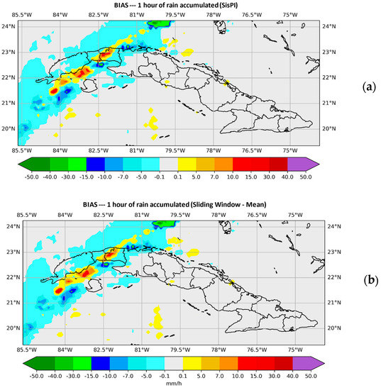
Figure 3. Plotted BIAS values. (a) shows those provided by SisPI in the forecast period (10–11) with the initialization at 12:00 UTC and (b) shows those provided by SisPI once the window method was applied with the average instruction for a window width N = 3.

In Figure 3a, SisPI errors are observed in the forecast period (10–11) with the initialization of 12:00 UTC, and in Figure 3b those are obtained once the window method is applied, with the mean instruction and for a window width N = 3. It can be seen by analyzing the figure that the forecast improvement in terms of precipitation amount errors is quite small, practically imperceptible.

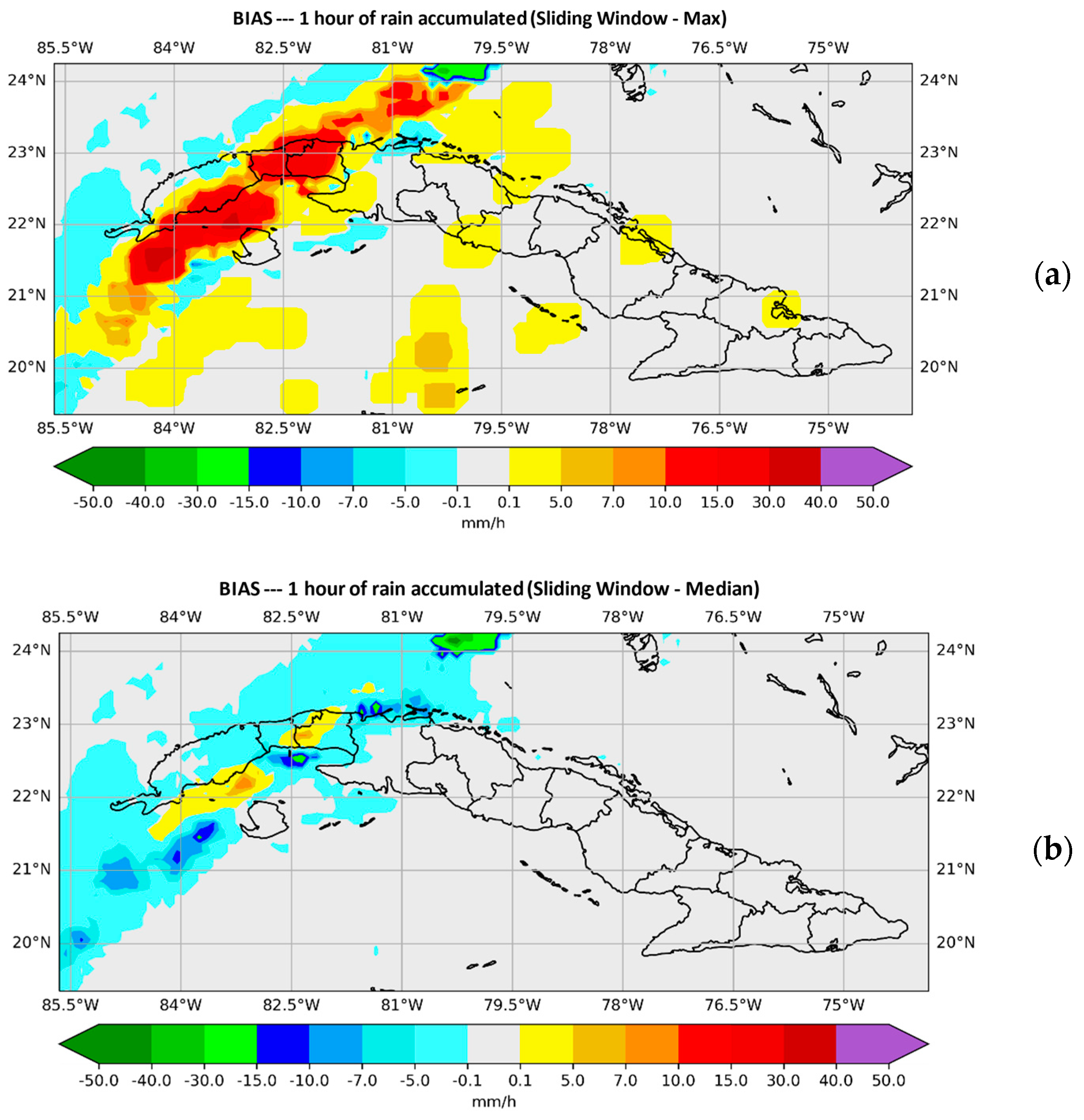
Figure 4 shows the plotted values of the BIAS. In Figure 4a the SisPI is shown once the method has been applied with the maximum instruction and in Figure 4b with the median instruction for the same forecast term (both for a window width N = 3). It can be observed that the maximum instruction overestimates the amount of precipitation, showing errors of even 30 mm of precipitation in 1 hour. Figure 4b shows how using the method with the window width N = 3 and the medium instruction, the magnitude with which the instruction decreases the precipitation amount errors is quite small, as was the case with the mean instruction (Figure 3b).

Figure 4. Plotted values of the BIAS. (a) shows those provided by the SisPI once the method was applied with the maximum instruction in the forecast period (10–11) with the initialization of the 12:00 UTC and in (b) the ones provided by SisPI with the median instruction and the same initialization, both images refer to the method with a window width N = 3.

With window size N = 15, Figure 5 and Figure 6, show the behavior of the BIAS for each of the instructions used. On this occasion, a clear improvement is observed with the median, while with the maximum, a spatial and quantitative overestimation of precipitation is observed.

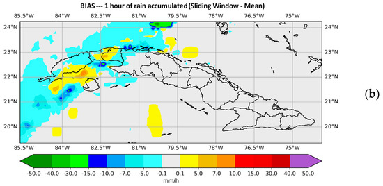
Figure 5. Plotted BIAS values. (a) shows those provided by SisPI in the forecast period (10–11) with the initialization at 12:00 UTC and (b) shows those provided by SisPI once the window method was applied with the average instruction. for a window size N = 15.

Figure 6. Plotted values of the BIAS, in (a) those provided by the SisPI are shown once the method has been applied with the maximum instruction and in (b) those provided by SisPI with the median instruction, both images for a window width N = 15 in the forecast period (10–11) with the initialization of 12:00 UTC.

4. Conclusions

The development of this research allowed us to reach the following conclusions:

• It was possible to reduce the spatial error by using a window of size N = 15 and the maximum and mean instructions.
• Regarding the quantitative error, it was possible to reduce it more optimally with the mean instruction, using the same window size.
• Instruction mean was the one that improved the precipitation forecast provided by SisPI in a most complete way, improving not just the spatial accuracy but also the amount of forecast precipitation.

References

- Yan, H.; Gallus, W.A. NAM, and GFS Models Using Multiple Verification Methods over a Small Domain; Department of Geological and Atmospheric Sciences, Iowa State University: Ames, Iowa, 2016. [Google Scholar]
- INSMET. INSMET MODELS. Available online: https://models.insmet.cu (accessed on 27 March 2021).
- BenYahmed, Y.; Bakar, A.A.; RazakHamdan, A.; Ahmed, A.; Abdullah, S.M.S. Adaptive Sliding window algorithm for weather data segmentation. J. Theor. Appl. Inf. Technol. 2015, 80, 332–333. [Google Scholar]
- Lorenzo, M.S.; Hernández, A.L.F.; Valdés, R.H.; Mayor, Y.G.; Rodríguez, R.C.G.; Montejo, I.B.; Gernó, C.F.R. Automatic Mesoscale Prediction System of Four Daily Cycles; Institute of Meteorology of Cuba, Center for Physics of the Atmosphere: Havana, Cuba, 2014. [Google Scholar]
- NASA. Available online: https://www.nasa.gov (accessed on 5 August 2020).
Publisher’s Note: MDPI stays neutral with regard to jurisdictional claims in published maps and institutional affiliations. |
© 2022 by the authors. Licensee MDPI, Basel, Switzerland. This article is an open access article distributed under the terms and conditions of the Creative Commons Attribution (CC BY) license (https://creativecommons.org/licenses/by/4.0/).