First- and Second-Order Sensitivities of Steady-State Solutions to Water Distribution Systems ^†

Abstract

First-order approximations have been used with some success for criticality analysis; sensitivity analysis of physical networks, such as water distribution systems; and uncertainty propagation of model parameters. Certain limitations have been reported regarding the accuracy of the results, particularly when non-linearity is dominant. In this paper, we show how to efficiently derive the first- and second-order sensitivities with respect to variation in their parameters. This makes it possible to improve the first-order estimate when necessary. The method is illustrated on a small example system.

1. Introduction

Water distribution systems (WDSs) are complex and aging. They need to be protected and made more resilient to natural and man-made disasters. There are considerable preservation, health and safety, and sustainability issues at stake in being able to properly manage and understand the operation of such systems.

Modelling tools can be very useful for handling such complex systems and for making sustainable management and crisis response decisions. Nevertheless, this may require solving optimization problems using large hydraulic digital models and may prove impossible to solve due to the curse of dimensionality. In response, some authors have suggested (1) using first-order estimates (e.g., the graph Laplacian matrix) [1,2], or (2) using graph partitioning and reduced-order models [3,4] to make these problems tractable. Depending on the problem under consideration, sub-optimality or some kind of limitation may be reported, particularly when precision is required for decision-making and non-linearity is important.

In addition, uncertainty in the input parameters requires the digital model to be combined with real-time observations to reduce the uncertainty of the output. Consequently, three main challenges in real-time modeling are (1) reducing the computational time, (2) quantifying uncertainties, and (3) coupling numerical models with observations. The sensitivity of steady-state solutions to variations in the model parameters provides a way to solve the first two challenges [5,6,7].

In this research, we show how to derive the first- and second-order sensitivities of model outputs to variations in the parameters by solving linear systems additional to the global gradient algorithm solution. First, we derive explicit formulae for the first- and second-order sensitivities to the parameters. Next, we describe an efficient and low-cost implementation, which uses the Cholesky decomposition of the Schur matrix to calculate the sensitivities. Finally, an illustrative example is used to show the potential application of hydraulic modeling to water distribution networks.

2. Methods

The method consists of observing that the following general conservation form system can be used to calculate the first- and second-order sensitivities of q (flow rate) and h (head) with respect to the parameters

$$\mathbf{F}{\mathbf{q}}_{\mathit{x}\mathit{y}}-\mathbf{A}{\mathbf{h}}_{\mathit{x}\mathit{y}}=\mathbf{x},$$

(1)

$$-{\mathbf{A}}^T{\mathbf{q}}_{\mathit{x}\mathit{y}}-\mathbf{E}{\mathbf{h}}_{\mathit{x}\mathit{y}}=\mathbf{y}.$$

(2)

$\mathbf{F}={\nabla }_q\mathsf{\xi }\in {\mathbb{R}}^{np,np}$ is the Jacobian of the head loss function$\mathsf{\xi }$; $\mathbf{A}\in {\mathbb{R}}^{np,nj}$ is the junction node-arc incidence matrix; $\mathbf{E}={\nabla }_h\mathbf{c}\in {\mathbb{R}}^{nj,nj}$ is the Jacobian of the pressure outflow relationship (POR) function c (for the demand-driven modeling (DDM) case, $\mathbf{E}=\mathbf{0}$); $\mathbf{x}\in {\mathbb{R}}^{np,nx}$ and $\mathbf{y}\in {\mathbb{R}}^{nj,ny}$ are appropriate vectors or matrices that are specified in Table 1; and ${\mathbf{q}}_{\mathit{x}\mathit{y}}$ are the flow-rate related quantities, ${\mathbf{h}}_{\mathit{x}\mathit{y}}$ are the head-related quantities).

Table 1. The right-hand sides for system (1–2) and their application.

Application	x	y	${\mathbf{q}}_{\mathit{x}\mathit{y}}$	${\mathbf{h}}_{\mathit{x}\mathit{y}}$
Hydraulic state from the linearized system	e a	${\mathbf{0}}_{nj}$	qlin	hlin
1st-order sensitivities with respect to demand	${\mathbf{0}}_{np,nj}$	${\nabla }_d\mathbf{c}$	${\nabla }_d\mathbf{q}$	${\nabla }_d\mathbf{h}$
$1^{\mathrm{st}}-\mathrm{order}\mathrm{sensitivities}\mathrm{with}\mathrm{respect}\mathrm{to}\theta ,$ defined in b	${-\nabla }_{\theta }\mathsf{\xi }$	${\mathbf{0}}_{nj,ny}$	${\nabla }_{\theta }\mathbf{q}$	${\nabla }_{\theta }\mathrm{h}$
2nd-order sensitivities with respect to demand	$\left(-{\displaystyle \frac{{\partial }^2{\xi }_j}{{\partial q_j}^2}}{\displaystyle \frac{{\partial q}_j}{\partial d_m}}{\displaystyle \frac{{\partial q}_j}{\partial d_n}}\right)$	$\left({\displaystyle \frac{{\partial }^2{c}_i}{{\partial h_i}^2}}{\displaystyle \frac{{\partial h}_i}{\partial d_m}}{\displaystyle \frac{{\partial h}_i}{\partial d_n}}+{\displaystyle \frac{E_{ii}}{d_i}}\left({\delta }_{in}{\displaystyle \frac{{\partial h}_i}{\partial d_m}}+{\delta }_{im}{\displaystyle \frac{{\partial h}_i}{\partial d_n}}\right)\right)$	$\left({\displaystyle \frac{{\partial }^2{q}_j}{\partial d_m\partial d_n}}\right)$	$\left({\displaystyle \frac{{\partial }^2{h}_i}{\partial d_m\partial d_n}}\right)$
2nd-order sensitivities with respect to theta	$\left(-{\displaystyle \frac{{\partial }^2{\xi }_j}{{\partial q_j}^2}}{\displaystyle \frac{{\partial q}_j}{\partial {\theta }_m}}{\displaystyle \frac{{\partial q}_j}{\partial {\theta }_n}}-{\displaystyle \frac{{\partial F}_{jj}}{{\partial r}_j}}\left({\displaystyle \frac{{\partial r}_j}{\partial {\theta }_n}}{\displaystyle \frac{{\partial q}_j}{\partial {\theta }_m}}+{\displaystyle \frac{{\partial r}_j}{\partial {\theta }_m}}{\displaystyle \frac{{\partial q}_j}{\partial {\theta }_n}}\right)\right)$	$\left({\displaystyle \frac{{\partial }^2{c}_i}{{\partial h_i}^2}}{\displaystyle \frac{{\partial h}_i}{\partial {\theta }_m}}{\displaystyle \frac{{\partial h}_i}{\partial {\theta }_n}}\right)$	$\left({\displaystyle \frac{{\partial }^2{q}_j}{\partial {\theta }_m\partial {\theta }_n}}\right)$	$\left({\displaystyle \frac{{\partial }^2{h}_i}{\partial {\theta }_m\partial {\theta }_n}}\right)$

^a Vector e represents the energy available from the source and resource nodes. It is defined as $\mathbf{e}={\mathbf{A}}_{\mathbf{0}}{\mathbf{h}}_{\mathbf{0}}$. ^b where ${\theta }_j$ is a characteristic parameter of pipe j, such as resistance factor, diameter, or relative roughness.

Indeed, system (1–2) is generic, as can be seen in Table 1. If we choose $\mathbf{x}=\mathbf{e}$ and $\mathbf{y}={\mathbf{0}}_{nj}$, system (1–2) is the linearized system of pressure-driven modeling (PDM) equations, and ${\mathbf{q}}_{\mathit{x}\mathit{y}}$ and ${\mathbf{h}}_{\mathit{x}\mathit{y}}$ are the estimates of q and h when the head loss and POR models are linear. Likewise, if $\mathbf{x}={\mathbf{0}}_{np,nj}$ and $\mathbf{y}={\nabla }_d\mathbf{c}$, then ${\mathbf{q}}_{\mathit{x}\mathit{y}}={\nabla }_d\mathbf{q}$ and ${\mathbf{h}}_{\mathit{x}\mathit{y}}{=\nabla }_d\mathbf{h}$ (see [7] for the derivation). Also, for differentiation with respect to${\theta }_j=r_j\mathrm{or}{D}_j\mathrm{or}{\epsilon }_j/D_j$ ($r_j$ = the resistance factor; $D_j$ = the pipe diameter; ${\epsilon }_j$/$D_j$ = the relative roughness of pipe j), the first-order sensitivities with respect to $\mathsf{\theta }$ are solutions of (1–2). Just choose $\mathbf{x}={-\nabla }_{\theta }\mathsf{\xi }$ and $\mathbf{y}={\mathbf{0}}_{nj,ny}$ (also derived in [7]).

We now consider double scalar differentiation with $d_m$ and then $d_n$ (respectively, ${\theta }_m$ and then ${\theta }_n$); system (1–2) can then be used to calculate the second-order sensitivities with appropriate choices of x and y, as shown in Table 1. The meaning behind this property is that the flows and heads with their derivatives share similar spatial structures or patterns.

Multiplying Equation (1) by ${\mathbf{A}}^T{\mathbf{F}}^{-1}$ and adding it to Equation (2) gives

$${\mathbf{h}}_{\mathit{x}\mathit{y}}={-\left({\mathbf{A}}^T{\mathbf{F}}^{-1}\mathbf{A}+\mathbf{E}\right)}^{-1}({\mathbf{A}}^T{\mathbf{F}}^{-1}\mathbf{x}+\mathbf{y}),$$

(3)

It follows from (1) that

$${\mathit{q}}_{\mathit{x}\mathit{y}}={\mathbf{F}}^{-1}(\mathbf{A}{\mathbf{h}}_{\mathit{x}\mathit{y}}+\mathbf{x}).$$

(4)

Equations (3) and (4) provide a solution template for a linearized estimate of q and h and the corresponding first-order and second-order sensitivities.

Equation (3) requires the solution of a symmetric matrix equation with the form

$$\left({\mathbf{A}}^T{\mathbf{F}}^{-1}\mathbf{A}+\mathbf{E}\right)\mathbf{z}=\mathbf{w}.$$

(5)

This is true for the calculation of all the sensitivities discussed here. If the sensitivities of the solutions to more than one parameter are required, then a significant computational economy can be made. Suppose a first solution is computed using the Cholesky factorization $\mathbf{L}{\mathbf{L}}^T$ = $\left({\mathbf{A}}^T{\mathbf{F}}^{-1}\mathbf{A}+\mathbf{E}\right)$. Sensitivity calculations for any other parameters can be solved with about $2n^2$ floating-point operations each rather than the full Cholesky cost of $\mathrm{O}\left(n^3/6\right)$ if the same L factor is used with forward and backward substitutions. In addition, further savings can be made by exploiting the sparsity of the Cholesky factor.

The solution of Equations (3) and (4) in this paper was coded with Matlab 2023b. The first- and second-order sensitivities can be calculated for a specific component vector or selected values of interest. This is what we propose in the results. Meanwhile, it is possible to organize the calculation if we are interested in obtaining an overall view. For example, for the second-order sensitivities of q with respect to all the demands, there are nj symmetrical matrices ${\mathbf{V}}_{\mathit{d}\mathit{k}}^{\mathit{q}}$, each with dimensions of $np\times nj$. Each matrix gives the second-order sensitivities of all the flows with respect to all the demands and one single demand. Thus, for example, the matrix for the sensitivities of flows $q_1,q_2,\dots ,q_{nj}$ to $d_k$ and all of $d_1,d_2,\dots ,d_{nj}$ has the following structure:

$${\mathbf{V}}_{{\mathit{d}}_{\mathit{k}}}^{\mathit{q}}=\left(\begin{array}{ccccccc}{\displaystyle \frac{{\partial }^2{q}_1}{\partial d_k\partial d_1}}& \cdots & {\displaystyle \frac{{\partial }^2{q}_1}{\partial d_k\partial d_{k-1}}}& {\displaystyle \frac{{\partial }^2{q}_1}{\partial d_k^2}}& {\displaystyle \frac{{\partial }^2{q}_1}{\partial d_k\partial d_{k+1}}}& \cdots & {\displaystyle \frac{{\partial }^2{q}_1}{\partial d_k\partial d_{n_j}}}\\ {\displaystyle \frac{{\partial }^2{q}_2}{\partial d_k\partial d_1}}& \cdots & {\displaystyle \frac{{\partial }^2{q}_2}{\partial d_k\partial d_{k-1}}}& {\displaystyle \frac{{\partial }^2{q}_2}{\partial d_k^2}}& {\displaystyle \frac{{\partial }^2{q}_2}{\partial d_k\partial d_{k+1}}}& \cdots & {\displaystyle \frac{{\partial }^2{q}_2}{\partial d_k\partial d_{n_j}}}\\ ⋮& & ⋮& ⋮& ⋮& & ⋮\\ {\displaystyle \frac{{\partial }^2{q}_{np}}{\partial d_k\partial d_1}}& \cdots & {\displaystyle \frac{{\partial }^2{q}_{np}}{\partial d_k\partial d_{k-1}}}& {\displaystyle \frac{{\partial }^2{q}_{np}}{\partial d_k^2}}& {\displaystyle \frac{{\partial }^2{q}_{np}}{\partial d_k\partial d_{k+1}}}& \cdots & {\displaystyle \frac{{\partial }^2{q}_{n_p}}{\partial d_k\partial d_{n_j}}}\end{array}\right)$$

3. Results

The network used to illustrate the application is shown in Figure 1. The Darcy–Weisbach head loss model and the one-side regularized Wagner POR model with a regularization parameter = 1/10 from [7] were used. The demand at node 1 was increased by 5, 10, 20, and 40 L/s. The second-order Taylor polynomial approximations to q and h around point $d_1$ are given by $\mathrm{X}\left(d_1+\delta \right)=\mathrm{X}\left(d_1\right)+{\displaystyle \frac{\partial X}{\partial d_1}}\delta +{\displaystyle \frac{1}{2!}}{\displaystyle \frac{{\partial }^2\mathrm{X}}{\partial d_1^2}}{\delta }^2.$ The results for the heads at the junction nodes and the flow rates are reported in Table 2. We can see the second-order estimates are not significantly different from the exact values in column 3.

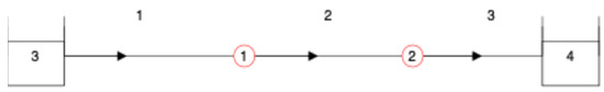
Figure 1. Example system with 2 tanks (nodes 3 and 4), 2 junction nodes (nodes 1 and 2) and 3 pipes. Pipe lengths are 1000 m; diameters are 250 mm; pipe roughnesses are 0.25 mm; source heads are both 100 m; junction node elevations are all 0; initial demand at node 1 (and, respectively, node 2) is 60 L/s (resp., 50 L/s).

Table 2. First- and second-order estimates for the example network with a demand perturbation of 40 L/s.

Name	h(d1)	h(d1 + 40)	$\mathbf{\partial }\mathit{X}\mathbf{/}\partial {\mathit{d}}_{\mathbf{1}}$	${\mathbf{\partial }}^{\mathbf{2}}\mathbf{X}\mathbf{/}{\partial {\mathbf{d}}_{\mathbf{1}}}^{\mathbf{2}}$	1st order Est.	Error in m	2nd order Est.	Error in m
Node 1	94.64	89.72	−0.099382	−0.001223	90.67	−0.95	89.69	0.03
Node 2	94.70	90.71	−0.089746	−0.000450	91.11	−0.40	90.75	−0.04
	q (d1)	q (d1 + 40)	$\mathbf{\partial }\mathit{X}\mathbf{/}\partial {\mathit{d}}_{\mathbf{1}}$	${\mathbf{\partial }}^{\mathbf{2}}\mathbf{X}\mathbf{/}{\partial {\mathit{d}}_{\mathbf{1}}}^{\mathbf{2}}$	1st order Est.	Error in L/s	2nd order Est.	Error in L/s
Pipe 1	55.14	76.94	0.524218	0.001617	76.11	0.83	77.41	−0.47
Pipe 2	−4.86	−23.06	−0.475782	0.001617	−23.89	0.83	−22.59	−0.47
Pipe 3	−54.86	−73.06	−0.475782	0.001617	−73.89	0.83	−72.59	−0.47

4. Discussion and Conclusions

In this paper, the same generic conservative-form system is used to derive linearized estimates of the flow and head and the first-order and, for the first time, second-order sensitivities. The right-hand sides of the governing equations change appropriately. Explicit formulae are given, and the fact that the same Cholesky factor and sparse solution matrix are shared explains why significant savings can be made in the calculation. It is possible to extend the method to higher-order sensitivities.

The development presented in this paper is useful for assessing the probability distributions for link flow rates and nodal piezometric heads. Additionally, it permits Taylor approximation for q and h around known working points. This opens the way to solving difficult problems using quadratic approximation or to speeding up extended-period simulations by improving the initial guesses.

References

- Abraham, E.; Blokker, E.J.M.; Stoianov, I. Network Analysis, Control Valve Placement and Optimal Control of Flow Velocity for Self-Cleaning Water Distribution Systems. Procedia Eng. 2017, 186, 576–583. [Google Scholar] [CrossRef]
- Steffelbauer, D.B.; Deuerlein, J.; Gilbert, D.; Abraham, E.; Piller, O. Pressure-Leak Duality for Leak Detection and Localization in Water Distribution Systems. J. Water Resour. Plan. Manag. 2022, 148, 04021106. [Google Scholar] [CrossRef]
- Elhay, S.; Deuerlein, J.; Piller, O.; Simpson, A.R. Graph Partitioning in the Analysis of Pressure Dependent Water Distribution Systems. J. Water Resour. Plan. Manag. 2018, 144, 1–13. [Google Scholar] [CrossRef]
- Pecci, F.; Abraham, E.; Stoianov, I. Model Reduction and Outer Approximation for Optimizing the Placement of Control Valves in Complex Water Networks. J. Water Resour. Plan. Manag. 2019, 145, 04019014. [Google Scholar] [CrossRef]
- Fu, G.; Kapelan, Z.; Reed, P. Reducing the Complexity of Multiobjective Water Distribution System Optimization through Global Sensitivity Analysis. J. Water Resour. Plan. Manag. 2012, 138, 196–207. [Google Scholar] [CrossRef]
- Hutton, C.; Kapelan, Z.; Vamvakeridou-Lyroudia, L.; Savić, D. Dealing with Uncertainty in WDS Models: A Framework for Real-Time Modeling and Data Assimilation. J. Water Resour. Plan. Manag. 2014, 140, 169–183. [Google Scholar] [CrossRef]
- Piller, O.; Elhay, S.; Deuerlein, J.; Simpson, A. Local Sensitivity of Pressure-Driven Modeling and Demand-Driven Modeling Steady-State Solutions to Variations in Parameters. J. Water Resour. Plan. Manag. 2017, 143, 12. [Google Scholar]
Disclaimer/Publisher’s Note: The statements, opinions and data contained in all publications are solely those of the individual author(s) and contributor(s) and not of MDPI and/or the editor(s). MDPI and/or the editor(s) disclaim responsibility for any injury to people or property resulting from any ideas, methods, instructions or products referred to in the content. |
© 2024 by the authors. Licensee MDPI, Basel, Switzerland. This article is an open access article distributed under the terms and conditions of the Creative Commons Attribution (CC BY) license (https://creativecommons.org/licenses/by/4.0/).