Abstract
The numbers of vehicles on the roads has increased tremendously. Also, the number of roads that are constantly experiencing traffic jams during morning and evening peak hours has increased significantly, which calls for a better understanding of traffic stream characteristics and car-following models. Traffic stream macroscopic parameters (speed, flow, and density) could be estimated through a number of traffic-flow theory models. In order to collect accurate data regarding fundamental of traffic stream parameters, a traffic monitoring system is needed to present the data from different roads. In this study, a real-time traffic monitoring system is introduced for traffic macroscopic parameters estimation. The sensor network has been constructed using a set of linear fiber optic sensors. In order to validate the system for this study, the system was installed at MnROAD facility, Minnesota. Fiber optic sensor detects the propagated strains in highway pavement due to the vehicle movements through the changes of the laser beam characteristics. Traffic flow can be estimated by tracking the peak of each axle passed over the sensor or within the sensitivity area, time mean speed (TMS), and space mean speed (SMS). SMS can be estimated by the different times a vehicle arrived at the sensors. The density can be determined either by using fundamental traffic flow theory model or estimating the time that vehicles occupy the sensor layout. Real traffic was used to validate the sensor layout. The results show the capability of the system to estimate traffic stream characteristics successfully.
1. Introduction
The number of vehicles has increased tremendously on roads due to rapid economic growth and urbanization as traffic volume increases on highway networks, contributing to traffic congestion, vehicle accidents, traffic safety, energy consumption, economic impact due to fuel and time waste, and green gas emission [1,2,3]. To better understand and overcome the traffic volume increment problems, vehicle-to-vehicle (V2V) and vehicle-to-infrastructure (V2I) interactions must necessarily be studied [4]. Traffic flow theory plays a critical role in understanding V2V interactions through a set of macroscopic parameters, including flow (q, vph), density (k, vpkm), and speed (S, kmph). These parameters could be estimated by a process called traffic state estimation (TSE), where an accurate estimation of macroscopic parameters (q, k, and s) plays a central role in the success of the developed traffic management system to mitigate traffic congestion problems [1]. Furthermore, TSE is vital for traffic planning (infrastructure management, maintenance) and traffic management (traffic control, ramp metering) [5].
Currently, the collected traffic data type can be sorted into two categories based on the measurement method: stationary data collected through fixed detectors, including loop detectors, inductive loops, closed-circuit television cameras (CCTV), fiber optic sensors [5,6,7,8]; and mobile data, such as on-vehicle GPS probe, OBD2, mounted video cameras, mobile phone, connected vehicle [5,9]. Despite expanding the use of mobile-collected data recently, it has problems with sampling and shows the potential for biases [5]. However, stationary collected data through fixed sensors represents every vehicle at their installed locations.
Fiber optic sensors have become widely accepted in traffic management and operation [10,11]. Fiber Bragg Grating (FBG) sensors are preferred among fiber optic sensors due to the distinctive characteristics that give them superiority over counterparts from other fixed sensors, including good linearity in response, accurate output, high resolution, small size, and low cost [12]. However, FBG sensors must be packaged since they are made of fiberglass. Currently, glass fiber reinforced polymers (GFRPs) are used in several fields, such as oil and gas, the pipe industry, structural elements, and aerospace [13], which makes it promising to be used as FBG sensor package material. Thus, this study introduces a stationary system for traffic stream parameter estimation based on GFRP-FBG sensor layout.
2. Sensor Fundamental
FBG sensor detects propagated strains () in highway pavement due to vehicle movements through the changes in the laser beam characteristics, as shown in Equation (1) [14]:
where Op is the optical elasticity parameter, is the Bragg wavelength due to mechanical load and temperature, and is the Bragg wavelength from a compensation temperature sensor.
Figure 1 shows the developed GFRP-FBG sensor by Zhou et al. [15], which will be used in this study for traffic stream characteristics estimation. Figure 1a shows the longitudinal component of the sensor, which is designed to detect the propagated strain in the x-y coordination. Figure 1b illustrates the vertical component of the sensor to monitor vertical strain.
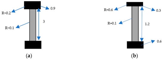
Figure 1.
GFRP-FBG sensor: (a) Longitudinal sensor; (b) Vertical component sensor. All units in (in.).
3. Methodology
To construct a traffic stream characteristics system, a minimum of two GFRP-FBG sensors must be installed along the road sequentially with a distance of (L) under the proposed vehicle tire track to increase the accuracy of the sensor measurements, with one FBG sensor to compensate for the temperature cross-sensitivity. Figure 2 shows the proposed sensor layout to estimate traffic macroscopic parameters, which consists of three GFRP-FBG sensors: a horizontal sensor (H-S), a vertical sensor(V-S) to track vehicle movement, and a horizontal temperature compensation sensor (H-TS). In this study, the distance L will be 4.87 m, which falls between the optimized distance interval from 2.13 m and 6.1 m to maximize the measurement accuracy for macroscopic parameters estimation.
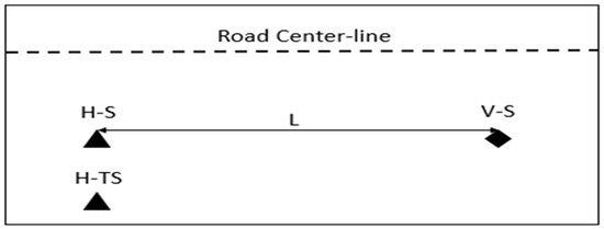
Figure 2.
Proposed sensor layout.
Estimating the traveled time for each passing vehicle between the two stationary sensors plays a vital role in deriving all macroscopic parameters (q, k, and s). Figure 3 illustrates the responses from the H-S sensor (positive measurement due to tension in the pavement along the road) and the V-S sensor (negative measurement due to compression at the location of the vertical sensor) for two consecutive vehicles (5 axle leading vehicles and 2 axle following vehicles).
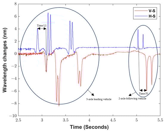
Figure 3.
Sensor’s response.
As noted in Figure 3, the sensor response will be more likely to have a peak shape due to the compact sensor’s size and higher vehicle speed, where each peak indicates the passing of one axle. Thus, the peaks will be tracked and counted accordingly for traffic flow (q) estimation, as stated in Equation (2). The recorded time (Time L1 and Time F1) indicates how long each vehicle travels over the known distance of (L) between the horizontal and the vertical sensors. Then, time mean speed (TMS) and space mean speed (SMS) can be calculated using Equations (3) and (4), respectively.
where N is the total number of vehicles in a period of time (T), and ti is the traveled time for a vehicle (i).
Therefore, density (k) can be calculated using the fundamental flow–density relationship, as follows:
4. Results and Discussion
To validate the system for traffic stream macroscopic estimation, the sensor layout was installed at the Cold Weather Road Research Facility in Minnesota (MnRoad) in Mn, USA. MnROAD consists of 50 test sections distributed on two roadways: a low-volume loop operated by 5 axle semi-truckand a section of (I-94) that contains two lanes operated by live traffic. The proposed sensor layout (Figure 2) was installed inside cell 17, part of I-94 at MnROAD, as shown in Figure 4.
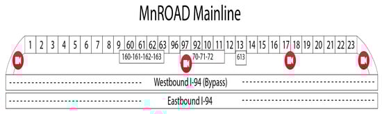
Figure 4.
MnROAD test section [16].
After the installation, the sensors were connected to a high-resolution integrator and personal computer to collect data. Figure 5 shows the response of both sensors (vertical and horizontal) when subjected to real traffic for 140 s to validate the system. From Figure 5, a total of 11 vehicles were recorded and tracked by the system. Thus, the flow (q) could be estimated, as equal to 283 vph.
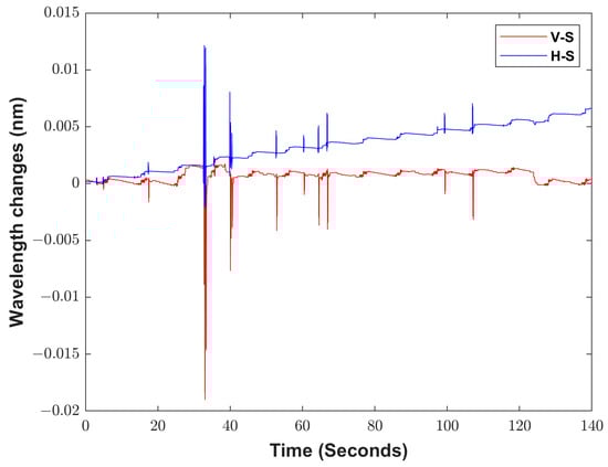
Figure 5.
Sensors’ response for 140 s.
Table 1 shows the estimated spot speed for the eleven vehicles recorded during 140 s, since the distance between sensors in the layout is defined (4.88 m). The system records the time at which the vehicle enters the sensor layout (Tin) and when the rear wheel exits the layout (Tout) to calculate the travel time for each vehicle, as shown in Table 1. Then, TMS, SMS, and K can be calculated using Equations (2)–(4), respectively. Therefore, TMS equals to 110.00 km\h, SMS equals 108.74 km\h, and k equals to 2.6 v/km.

Table 1.
Estimated spot speed.
5. Conclusions
This study successfully introduces a traffic stream characteristics estimation system based on an in-pavement sensor layout. The developed system will be durable since the sensors are packaged in GFRP material. The number of passed vehicles are tracked and counted for traffic flow estimation; with a higher sampling rate, the travel time of each vehicle is recorded with high accuracy. Then, speed (TMS and SMS) is estimated with previous knowledge of the distance between sensors. Future efforts will be applied to estimate traffic microscopic parameters (headway and spacing).
Funding
This research received no external funding.
Institutional Review Board Statement
Not applicable.
Informed Consent Statement
Not applicable.
Data Availability Statement
Available upon request.
Acknowledgments
The author would like to thank MnROAD technicians who helped during field testing.
Conflicts of Interest
The author declares no conflicts of interest.
References
- Xing, J.; Wu, W.; Cheng, Q.; Liu, R. Traffic State Estimation of Urban Road Networks by Multi-Source Data Fusion: Review and New Insights. Phys. A Stat. Mech. Its Appl. 2022, 595, 127079. [Google Scholar] [CrossRef]
- Abbas, Z.; Al-Shishtawy, A.; Girdzijauskas, S.; Vlassov, V. Short-Term Traffic Prediction Using Long Short-Term Memory Neural Networks. In Proceedings of the 2018 IEEE International Congress on Big Data (BigData Congress), San Francisco, CA, USA, 2–7 July 2018; pp. 57–65. [Google Scholar]
- Zhou, X.; Tanvir, S.; Lei, H.; Taylor, J.; Liu, B.; Rouphail, N.M.; Frey, H.C. Integrating a Simplified Emission Estimation Model and Mesoscopic Dynamic Traffic Simulator to Efficiently Evaluate Emission Impacts of Traffic Management Strategies. Transp. Res. Part D Transp. Environ. 2015, 37, 123–136. [Google Scholar] [CrossRef]
- Asaithambi, G.; Kanagaraj, V.; Srinivasan, K.K.; Sivanandan, R. Study of Traffic Flow Characteristics Using Different Vehicle-Following Models under Mixed Traffic Conditions. Transp. Lett. 2018, 10, 92–103. [Google Scholar] [CrossRef]
- Seo, T.; Bayen, A.M.; Kusakabe, T.; Asakura, Y. Traffic State Estimation on Highway: A Comprehensive Survey. Annu. Rev. Control. 2017, 43, 128–151. [Google Scholar] [CrossRef]
- Kwon, J.; Varaiya, P.; Skabardonis, A. Estimation of Truck Traffic Volume from Single Loop Detectors with Lane-to-Lane Speed Correlation. Transp. Res. Rec. 2003, 1856, 106–117. [Google Scholar] [CrossRef]
- Asmaa, O.; Mokhtar, K.; Abdelaziz, O. Road Traffic Density Estimation Using Microscopic and Macroscopic Parameters. Image Vis. Comput. 2013, 31, 887–894. [Google Scholar] [CrossRef]
- Won, M. Intelligent Traffic Monitoring Systems for Vehicle Classification: A Survey. IEEE Access 2020, 8, 73340–73358. [Google Scholar] [CrossRef]
- Li, H.; Qin, L.; Chang, X.; Rong, J.; Ran, B.; Jia, L. Sensor Layout Strategy and Sensitivity Analysis for Macroscopic Traffic Flow Parameter Acquisition. IET Intell. Transp. Syst. 2017, 11, 212–221. [Google Scholar] [CrossRef]
- Huang, M.-F.; Salemi, M.; Chen, Y.; Zhao, J.; Xia, T.J.; Wellbrock, G.A.; Huang, Y.-K.; Milione, G.; Ip, E.; Ji, P. First Field Trial of Distributed Fiber Optical Sensing and High-Speed Communication over an Operational Telecom Network. J. Light. Technol. 2019, 38, 75–81. [Google Scholar] [CrossRef]
- Liu, H.; Ma, J.; Yan, W.; Liu, W.; Zhang, X.; Li, C. Traffic Flow Detection Using Distributed Fiber Optic Acoustic Sensing. IEEE Access 2018, 6, 68968–68980. [Google Scholar] [CrossRef]
- Guo, H.; Xiao, G.; Mrad, N.; Yao, J. Fiber Optic Sensors for Structural Health Monitoring of Air Platforms. Sensors 2011, 11, 3687–3705. [Google Scholar] [CrossRef] [PubMed]
- Landesmann, A.; Seruti, C.A.; de Miranda Batista, E. Mechanical Properties of Glass Fiber Reinforced Polymers Members for Structural Applications. Mater. Res. 2015, 18, 1372–1383. [Google Scholar] [CrossRef]
- Zhang, Z.; Huang, Y.; Palek, L.; Strommen, R. Glass Fiber–Reinforced Polymer–Packaged Fiber Bragg Grating Sensors for Ultra-Thin Unbonded Concrete Overlay Monitoring. Struct. Health Monit. 2015, 14, 110–123. [Google Scholar] [CrossRef]
- Zhou, Z.; Liu, W.; Huang, Y.; Wang, H.; Jianping, H.; Huang, M.; Jinping, O. Optical Fiber Bragg Grating Sensor Assembly for 3D Strain Monitoring and Its Case Study in Highway Pavement. Mech. Syst. Signal Process. 2012, 28, 36–49. [Google Scholar] [CrossRef]
- MnROAD Mainline Traffic Cameras. Available online: https://www.dot.state.mn.us/mnroad/operations/traffic-cameras.html (accessed on 20 December 2023).
Disclaimer/Publisher’s Note: The statements, opinions and data contained in all publications are solely those of the individual author(s) and contributor(s) and not of MDPI and/or the editor(s). MDPI and/or the editor(s) disclaim responsibility for any injury to people or property resulting from any ideas, methods, instructions or products referred to in the content. |
© 2023 by the author. Licensee MDPI, Basel, Switzerland. This article is an open access article distributed under the terms and conditions of the Creative Commons Attribution (CC BY) license (https://creativecommons.org/licenses/by/4.0/).