Time Series Modelling and Predictive Analytics for Sustainable Environmental Management—A Case Study in El Mar Menor (Spain) ^†

Abstract

In this study on data science and machine learning, time series analysis plays a key role in predicting evolving data patterns. The Mar Menor, located in the Region of Murcia, represents an urgent case due to its unique ecosystem and the challenges it faces. This paper highlights the need to study the environmental parameters of the Mar Menor and to develop accurate predictive models and a standardised methodology for time series analysis. These parameters, which include water quality, temperature, salinity, nutrients, chlorophyll, and others, show complex temporal variations influenced by different activities. Advanced time series models are used to gain insight into their behaviour and project future trends, facilitating effective conservation and sustainable development strategies. Models such as SARIMA and LSTM stand out as valid for predicting the environmental patterns of the Mar Menor.

1. Introduction

The Mar Menor is a coastal lagoon in the Region of Murcia (Spain) that faces a series of major environmental and ecological problems, which has generated the need to analyse and understand its evolution, as well as its indicators trend over time. Time series analysis in the context of the Mar Menor provides valuable information on the changes and dynamics of this lagoon. These data provide key information for data collection in the management and conservation of this ecosystem, as well as for the implementation of protection and restoration measures. However, time series analysis present distinctive challenges. They can be complex and influenced by factors as diverse as seasonal cycles, weather events, and human activities. In addition, there may be irregularities, missing data, and noise that make time series difficult to interpret and model. In this context, we aim to address these problems and provide an enhanced understanding of time series dynamics and existing patterns.

In the field of data science and machine learning, time series analysis plays a crucial role in studying and predicting data that evolve over time. The main objective of time series analysis is to understand its performance and predict its evolution, but there are a variety of approaches and algorithms available; different models have different assumptions, characteristics, and capabilities; and their performance can vary significantly.

Therefore, there is a need to identify a standard process for selecting predictive models appropriate to a time series characteristic, allowing the best approach to be identified for each situation, maximising model performance, and minimising prediction error. For this reason, time series characteristics that may have an influence on predictive models’ performance were analysed, including trend, seasonality, and time dependence.

Several approaches can be used for this purpose, ranging from classical statistical models such as autoregressive (AR), moving average (MA), autoregressive moving average (ARMA), autoregressive integrated moving average (ARIMA), or autoregressive integrated moving average with seasonality component (SARIMA) models, to models such as the Facebook Prophet or recurrent neural networks (RNNs), concretely, long short-term memory (LSTM) models.

The dataset employed in this paper comes from the Mar Menor Data Web, It consist in data derived from different monitoring stations along the Mar Menor lagoon, with a time interval of five years, from 2017 to 2022.

2. Materials and Methods

2.1. Mar Menor Dataset

The data on Mar Menor’s parameters provide essential information for management and conservation decisions in this ecosystem, as well as for implementing appropriate protection and restoration measures. From the Mar Menor Data Web, the downloaded data included a pretreatment as interpolation, which made these data easier to process. The parameters selected to study are: chlorophyll (mg/L), salinity (PSU), oxygen levels (mg/L), phycoerythrin (ppm), water temperature (°C), and transparency (m).

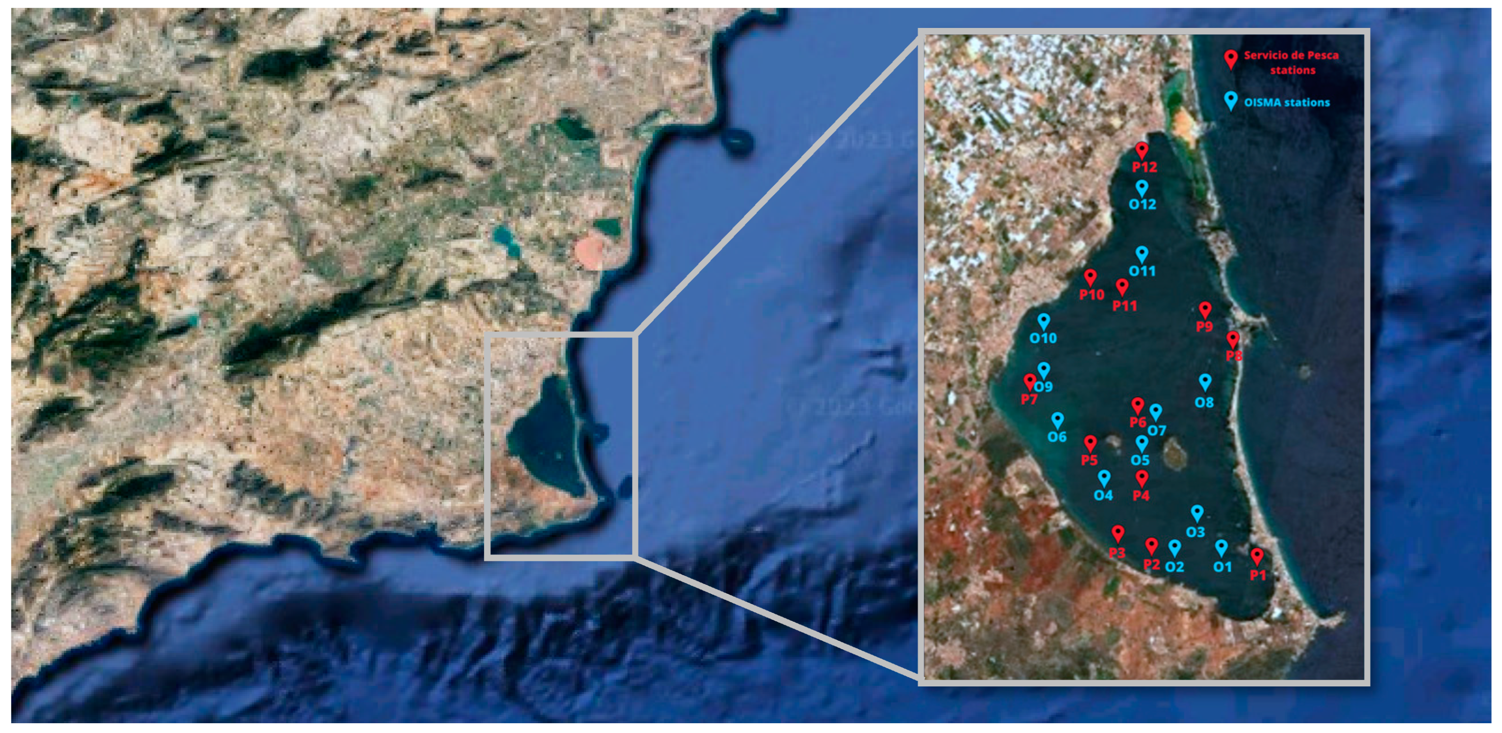
The time interval of these historical series was about 5 years, from 2017 to 2022. Data were extracted from different monitoring stations scattered throughout the Mar Menor and were subsequently standardised by the supplier to a common grid, as shown in Figure 1; OISMA (Oficina de Impulso Socioeconómico del Medio Ambiente) stations are shown in blue, and the Servicio de Pesca stations are shown in red.

2.2. Time Series and Machine Learning Models

Time series are sequential observations recorded at regular intervals and analysed for patterns or components such as trend or seasonality; in this context, the development of accurate and effective predictive models is essential to obtain reliable results. As mentioned in the Introduction, two approaches of time series analysis were evaluated to study the behaviour of different environmental parameters of the Mar Menor: statistical and machine learning models.

• Statistical models

Autoregressive models, moving average models, and a combination of the two were used. AR(p) models calculate future values with a linear combination of past values (p), which are determined by the partial autocorrelation function, where p is the order of the process indicating the number of previous time steps in the time series that are used to predict the future value of the series. In MA(q) models, the current value of a time series depends only on a small number of past values. This model calculates current values by first determining the average of past errors, achieved by summing them. Subsequently, these averaged values are multiplied by their respective coefficients to obtain the final results. Here, the model order (q) indicates the errors used to obtain the current value. A combination of the properties of the AR and MA processes was considered in which the stationarity of the time series was assumed. The resulting process is stochastic and stationary, called ARMA(p, q) [1]. In addition, there is an “integrated” version of a stationary series, called ARIMA(p,d,q); this model is considered stationary after differentiation. These are the most general classical models in time series forecasting, Where the parameter d represents the differencing order, which is the number of times the data series is differenced to achieve stationarity. Also, SARIMA models consider seasonal patterns and improve forecasting accuracy, and it is necessary to realise a deseasonalisation or seasonal difference (denoted by SARIMA(p,d,q)(P,D,Q), where P, D, and Q represent the seasonal autoregressive, the differencing order, and the moving average order, respectively [2]. Lastly, the Facebook Prophet model, based on the fitting curve technique of the Bayesian model, is appropriate when there is a large seasonality, and it is robust against missing data or trend variations. This model is a non-linear autoregressive additive model, with observations recorded hourly, daily, and monthly over a period of one year or more [3].

• Machine learning models

A recurrent neural network (RNN) is a type of artificial neural network that is specifically used for preprocessing sequential data or time series. These networks are designed to learn from new data and are distinguished by their ability to ‘remember’ past inputs. This memory informs their decision-making process, affecting both the intake of inputs and the generation of outputs. In fact, RNN results depend on the sequence of past elements, allowing time dependencies in the data to be captured. In this paper, a long short-term memory (LSTM) algorithm, a type of RNN with an input layer, an intermediate layer, and an output layer, was used to introduce different time series as input and to train the network with these data [4].

2.3. Methodology

The standardised process was based on a systematic and objective approach. Clear criteria and relevant evaluation metrics were used. A methodology was followed to guide users through the various steps, from initial exploration and data preprocessing to the selection and tuning of appropriate predictive models.

This methodology is structured into five phases: data cleaning and visualization, pattern identification, data transformation for model tuning, model selection and explanation of patterns, and finally, model implementation. In the first phase, a detailed examination of the time series was carried out with the aim of identifying trends and the possible missing data; thus, correction techniques such as interpolation or rolling averaging were used where necessary, and they did not affect the subsequent analysis. Erroneous data were removed, while original data providing useful information were kept. In the pattern identification phase, the Dickey–Fuller test assessed stationarity, assuming the null hypothesis that the series is non-stationary and the alternative hypothesis of stationarity. Partial autocorrelation analyzed seasonality. Transformation techniques, including differentiation and deseasonalization, were applied based on identified characteristics. Following the analysis of all time series, information criteria methods like Akaike (AIC) and Schwarz Bayesian (BIC) guided the selection of the most suitable model for each series, prioritizing those with the lowest AIC and BIC values. Finally, once the best model was selected, predictive models were applied to the series. For this, the dataset for the time series was split into training and testing sets in an 85/15 ratio. Predictions for statistical models were made using a predictive horizon of 7 and the training set was updated at each time step. Meanwhile, both the Facebook Prophet and LSTM models made predictions with a predictive horizon of 7 days on the entire 15% test set. Lastly, in order to assess the fitting of the models, several error metrics were implemented: root mean square error (RMSE), mean absolute error (MAE), and mean absolute percentage error (MAPE).

3. Application

Table 1. Size, range, and outliers of Mar Menor datasets.

Dataset	Total Data	Range	Outliers
Chlorophyll	975	06/2017–01/2020	47
Salinity	2041	04/2017–10/2022	0
Oxygen	1737	04/2017–12/2021	0
PE	487	07/2021–10/2022	22
Temperature	974	04/2017–11/2019	0
Transparency	2252	09/2016–10/2022	0

presents the results of the Mar Menor dataset. For clarity and relevance, only the phycoerythrin (PE) and water temperature (T) parameters are displayed as examples of the method’s implementation. In the data cleaning and visualization step, out of 1462 data points, 4.7% were removed due to being outliers, as shown in Table 1. This removal was part of the data processing which included interpolation, revealing that missing or atypical data did not significantly impact the results.

After data cleaning, pattern identification involved two key analyses. The first was the Dickey–Fuller test, which treated non-stationarity as the null hypothesis and stationarity as the alternative. The test was conducted with a 95% confidence threshold; a p-value above 0.05 implies rejection of the null hypothesis, indicating non-stationarity of the series. The second analysis focused on seasonality, using partial autocorrelation, where values above 0.5 were deemed significant. The outcomes of both analyses are detailed in

Table 2. Seasonality and stationarity for the different datasets.

Dataset	p-Value	Correlation Value
Chlorophyll	0.065	0.558
Salinity	0.067	0.824
Oxygen	0.055	0.692
PE	0.232	0.371
Temperature	0.072	0.818
Transparency	0.061	0.807

.

Based on the established criteria, it can be concluded that none of the datasets are stationary. Moreover, with the exception of the phycoerythrin (PE) data, there is an absence of seasonality in the other datasets. Subsequently, differentiation or deseasonalization techniques were employed to enhance the data’s compatibility with the models. This approach aimed to select the most appropriate model, thereby increasing estimation accuracy and reducing error rates.

To determine the best model, i.e., the model with the lowest value of AIC and BIC, we assessed different model fits by making combinations of the hyperparameters p and q, varying them from 0 to 4.

Table 3. The most appropriate statistical models for the Mar Menor datasets based on the AIC and BIC.

Dataset	Model	AIC	BIC
Chlorophyll	SARIMA(2,1,1) (0,1,1)	393.866	417.483
Salinity	SARIMA(3,1,2) (0,1,1)	−6482.535	−6443.294
Oxygen	SARIMA(2,1,3) (0,1,1)	−3023.798	−2985.705
PE	ARIMA(2,1,1)	−2418.08	−2401.08
Temperature	SARIMA(2,1,0) (0,1,1)	−1686.45	−1667.05
Transparency	SARIMA(1,1,2) (0,1,1)	−4900.312	−4871.730

presents the models obtained for each parameter and the lowest AIC and BIC values calculated. Thereby, predictions were made using these statistical models, in addition to the Facebook Prophet and LSTM models, which were applied to the dataset as well.

4. Results

Table 4. Error metrics for different models and datasets.

Dataset	Evaluation	Statistical Model	Facebook Prophet Model		LSTM Model
		Horizon 7	Horizon 7	15%	Horizon 7	15%
Chlorophyll	RMSE	2.420	4.377	5.621	9.63	6.431
	MAE	1.465	3.519	4.146	1.608	1.311
	MAPE	0.243	0.707	0.504	0.670	0.102
Salinity	RMSE	0.180	0.587	1.009	0.475	0.152
	MAE	0.134	0.488	0.840	0.550	0.359
	MAPE	0.003	0.012	0.021	0.028	0.008
Oxygen	RMSE	0.316	0.544	1.157	0.025	0.133
	MAE	0.214	0.435	1.014	0.116	0.315
	MAPE	0.036	0.078	0.184	0.198	0.058
PE	RMSE	0.170	0.334	0.333	0.009	0.002
	MAE	0.130	0.305	0.293	0.067	0.041
	MAPE	0.317	0.921	0.822	0.904	0.114
Temperature	RMSE	0.996	0.919	0.932	0.130	0.313
	MAE	0.697	0.743	0.758	0.277	0.499
	MAPE	0.032	0.036	0.035	0.256	0.019
Transparency	RMSE	0.219	1.153	3.060	0.037	0.018
	MAE	0.124	0.983	2.860	0.153	0.121
	MAPE	0.045	0.307	0.772	0.286	0.035

displays the outcomes of the prediction models. As previously noted, these models, including statistical models, Facebook Prophet, and LSTM, were used to make predictions over a 7-day horizon, applying 15% of the data as test data. The error metrics—RMSE, MAE, and MAPE—are detailed in Table 4. Additionally, Figure 2 visualizes these results, highlighting the predictions made using the most effective model for each dataset.

5. Conclusions

Firstly, this study highlights the significance of thoroughly comprehending the time series and clearly defining the analysis objectives. It identifies two crucial characteristics of time series analysis, emphasizing their essential role in understanding the data, minimizing errors, enhancing the accuracy of predictions, and preparing the data for deeper analysis. Furthermore, it’s vital to have a comprehensive understanding of both key performance and error metrics, alongside ensuring data cleanliness, to facilitate the selection of the most appropriate model.

In conclusion, the models generally yielded favorable prediction results, with the statistical and LSTM models emerging as the most effective for this data. Specifically, in the case of the PE data, the LSTM model achieved the lowest error, demonstrating an RMSE of 0.002 over a 7-day predictive horizon.

6. Discussion

The overall results and predictions of this study are positive, suggesting the applied methodology is effective. However, there were limitations regarding the forecasting horizons. Predictions beyond the selected horizon were not feasible with both statistical and machine learning models. While long-term estimations were unattainable with statistical models, machine learning models showed more promise in this regard. Additionally, the data preprocessing was relatively straightforward, benefiting from earlier processing and standardization via the server (L4 level).

One notable issue was the high error rates in chlorophyll predictions, attributable to the training data’s significant variance from the prediction data, starting with low values and increasing markedly towards the series’ end.