Short-Term Wind Forecasting in Adrar, Algeria, Using a Combined System ^†

Abstract

Forecasting wind speed using only one single model may not be satisfactory; however, the combination of several models may provide better results, especially in case of doubt about the best estimator (predicator). In this paper, we propose a short-term forecasting system in order predict the hourly averaged wind speed (HAWS) in the region of Adrar, Algeria. The proposed system is based on adaptive combination of two different models. The first model is an ARMA-based model, while the second model is an artificial neural network ANN-based model. To allow adaptive combination, models are associated to time varying coefficients that are updated recursively using the recursive least square algorithm (RLS). Numerical simulations have shown that for few hours in advance, the prediction error of the combined system is lower or at least equal to the best estimator.

1. Introduction

In wind energy industry, there is always some uncertainty about the final product due to the fact that wind speed is highly variable. The ability to predict wind speed for few hours in advance will help to ensure efficient utilization of the power generated, and therefore, enhance the position of wind energy compared to other forms of energy.

Forecasting of wind speed has been the subject of a lot of studies. Statistical and artificial neural networks are the approaches the most found in literature. Based on the hourly averaged wind speed (HAWS), several models have been developed using time series methodologies. In 1984, Geerts has proposed a short-term forecasting of wind speed using ARMA models [1]. A comparison of the performances of ARMA models developed using one-year data with those of the persistent model has indicated that for more than 1 h, ARMA models provide better forecasting. This shows that models developed using several years data could provide better results than those developed using only one-year data. Daniel and Chen (1991) have used a three-year long time series to develop ARMA models [2]. Since then, several similar studies have been realized for many sites around the world. Using 12-year data, Nfaoui et al. (1996) concluded that an AR(2) model is able to simulate the wind speed data of Tangiers (Morocco) [3]. Such methodologies have been confirmed by Kamal and Jafri (1997) using data of Quetta (Pakistan) [4]. Torres et al. (2004) used data of five locations in Navarre (Spain) to identify up to 10 different ARMA models [5].

Models based on artificial neural networks have been compared with ARMA models by Sfetsos (1999) [6]. Using only data of one month (March), the author has concluded that ANN models outperform the linear models. Using ANN and ARIMA models, More et al. (2003) have forecasted daily and monthly wind speed in India. Results indicate that performances of ANN models are better than ARIMA models [7]. Using one-month long data (January), Erasmo et al. (2009) concluded that for the particular case of La Venta (México), a model with two layers and three neurons was the best for training and forecasting [8].

In the following work, we propose HAWS forecasting systems based on adaptive combinations of two alternative (individual) models. The first model is based on ARMA approach, while the second is based on ANN approach. Adaptive combination is done by associating time-varying weights to the alternative models. The time-varying weights are adapted recursively using recursive least square algorithm (RLS). An important motive to combine forecasts from different models is the fundamental assumption that one model cannot identify the true process exactly, but different models may play a complementary role in the approximation of the data generating process, especially in case of doubt about the existence of the best estimator.

Data used in this work are measured over four years (November 2004 to October 2008) by the meteorological station situated at the airport of Adrar, Algeria (27.9° N, 0.3° W). Because of the gaps found in time series, our study is limited only for three months (January, November, and December). Data of the three first years are used to identify ARMA and train ANN models. The four-year data are used as an independent dataset to verify the forecasting ability of the obtained models.

2. ARMA Modeling

ARMA modeling for HAWS consists of three main steps: the first step is the power transformation which is done in order to carry the wind speed from Weibull distribution to Gaussian distribution [2]. The second step is the standardization step. The purpose of this step is to eliminate non-stationarity due to daily cyclical behaviors. The last step is the identification step which consists of the order determination and parameters estimation.

2.1. Power Transformation

For lot of sites over the word, it has been found that Weibull distribution (Equation (1)) fits the wind distribution the best:

$$f(v)=\frac{k}{c}{\left(\frac{v}{c}\right)}^{k-1}{e}^{-{\left(\frac{v}{c}\right)}^k}$$

(1)

where $v$ is the wind speed, $k$ is the form factor, and $c$ is the scale factor.

In order to fit ARMA models to the HAWS, power transformation of the observed data must be performed. The aim of the power transformation is to approximate the distribution of the wind data from a Weibull distribution to Gaussian one. The power transformation is performed by raising each value of the observed data by the same power index. For more accurate approximation, Daniel and Chen (1991) have proposed to use $x=k/3.6$ as a reference to obtain more accurate index $m$ using skewness statistics is given as [2]:

$$S_m={\displaystyle \sum _{y=1}^Y{\displaystyle \sum _{n=1}^N\frac{{\left[\left(v_{n,y}^m-mean(v_{n,y}^m)\right)/std(v)\right]}^3}{Y.N}}}$$

(2)

where $Y$ is the number of considered years and $N$ is the number of samples per month. After iterative calculations using several values of $m$, the selected $m$ is the one that makes distribution of $v^m$ symmetric i.e., $S_m\approx 0$. Values of Weibull parameters, of Dubey’s index x and asymmetry index m are evaluated for the three proposed months and presented in Table 1.

Table 1. Estimated parameters for the Weibull distribution and ARMA models.

Title 1	Month	C	K	$\mathit{x}$	$\mathit{m}$	ARMA	AR	MA
January	6.43	7.19	2.55	0.70	0.68	(3,0)	$ARMA(3,0)$ $\begin{array}{l}{\phi }_1=0.70\\ {\phi }_2=0.10\\ {\phi }_3=0.06\end{array}$
November	5.89	6.61	2.23	0.62	0.75	(3,0)	$\begin{array}{l}{\phi }_1=0.72\\ {\phi }_2=0.09\\ {\phi }_3=0.07\end{array}$	-
December	6.02	6.74	2.22	0.63	0.57	(3,0)	$\begin{array}{l}{\phi }_1=0.72\\ {\phi }_2=0.11\\ {\phi }_3=0.04\end{array}$	-

2.2. Standarisation

Diurnal non-stationarity can be eliminated by subtraction the hourly averaged wind speed u(t) from the transformed HAWS then dividing by the hourly standard deviation $s\left(t\right)$ [5]. Transformed and standardized HAWS (TS-HAWS) are given as:

$$v_{n,y}^{*}=(v_{n,y}^m-u(t))/s(t)$$

(3)

where

$$u(t)=\frac{{\displaystyle \sum _{y=1}^Y{\displaystyle \sum _{i=1}^d{v}_{y,i*24+t}^m}}}{Y*d}$$

(4)

and

$$s(t)=\sqrt{\frac{{\displaystyle \sum _{y=1}^Y{\displaystyle \sum _{i=1}^d{\left(v_{y,i*24+t}^m-u(t)\right)}^2}}}{Y*d}}$$

(5)

It is assumed that $u(t)$ and $s(t)$ are periodic functions, i.e., $u(1)=u(25)$, $u(2)=u(26)$, $s(1)=s(25)$, and $s(2)=s(26)$, where d is the number days for given month.

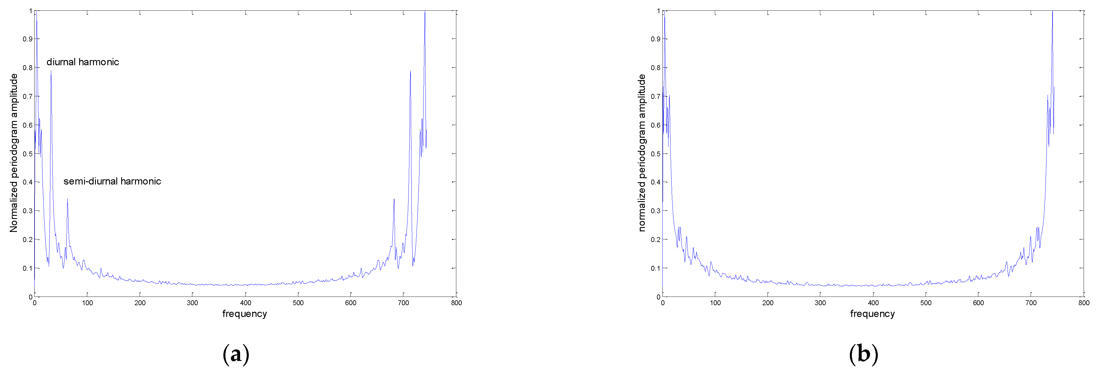
To illustrate the effect of standardization on HAWS, periodograms of original HAWS and TS-HASW are evaluated and presented in Figure 1. It is clear that diurnal and semidiurnal harmonics present in the periodogram of HAWS in the form of peaks have been canceled from the periodogram of the TS-HAW.

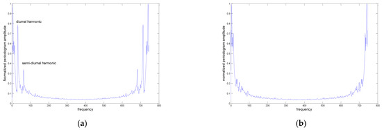
Figure 1. Periodograms of HAWS (a) and TS-HAWS (b).

2.3. ARMA Fitting

The following section consists of fitting ARMA models to TS-HAWS. A general model is given as:

$$\begin{array}{ll}{v}_{n,y}^{*}& =\left({\phi }_{1}L+{\phi }_2{L}^2+\cdots +{\phi }_p{L}^p\right)v_{n,y}^{*}\\ & +{\epsilon }_{n,y}\left(1-{\theta }_{1}L-{\theta }_2{L}^2-\cdots -{\theta }_q{L}^q\right)\end{array}$$

(6)

where p is the order of the autoregressive part, q is the order of the moving part, L is the lag operator, and $\epsilon$ is a white Gaussian noise of zero mean and variance ${\sigma }_{\epsilon }^2$.

2.3.1. Order Determination

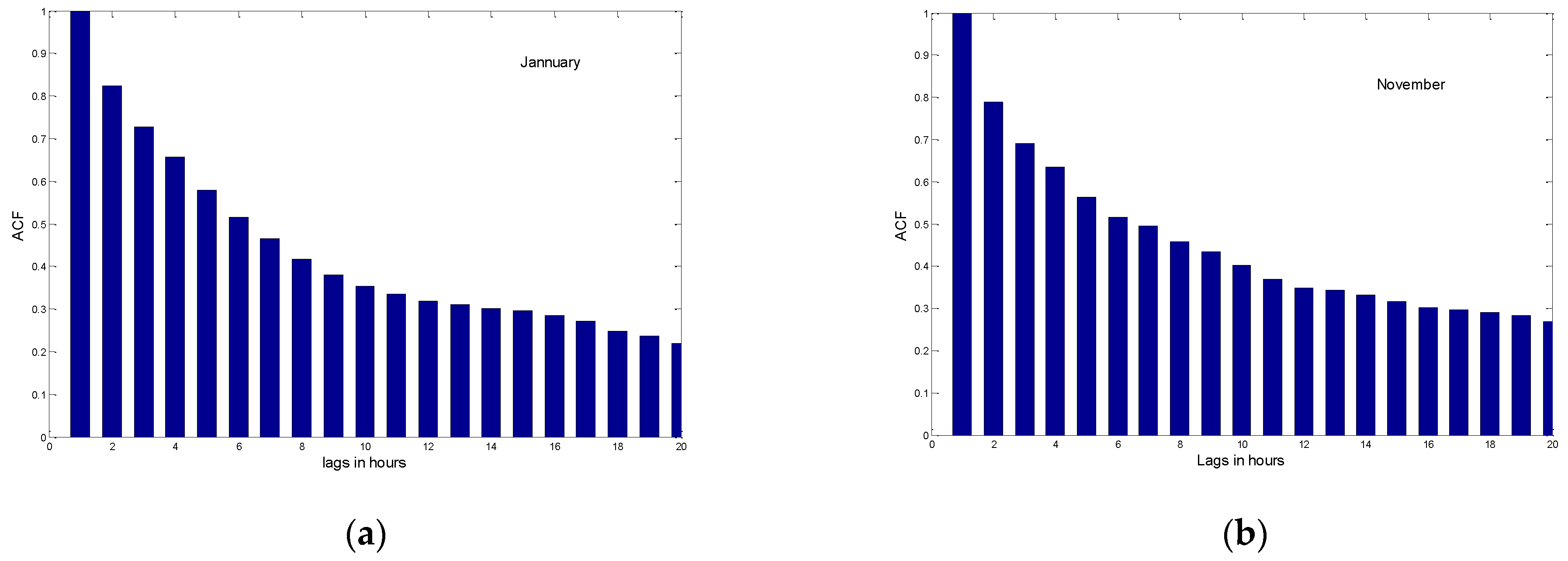
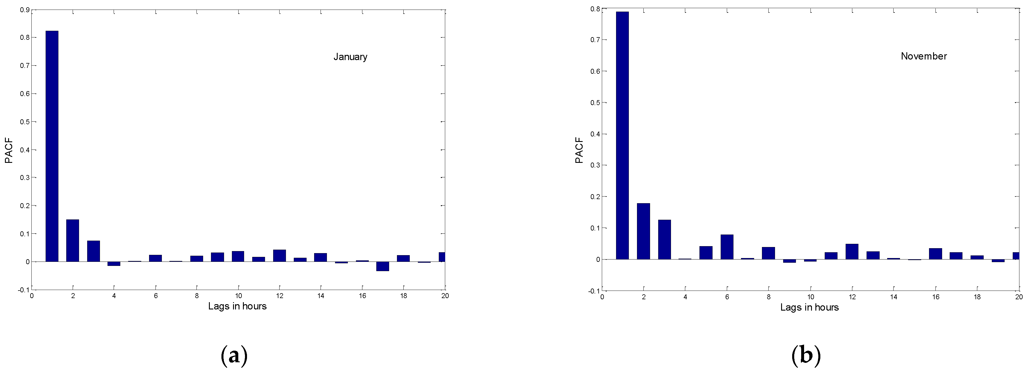
The following section consist of identifying the values of p and q. A pure MA process exhibits a cut of after q lags in the autocorrelation function (ACF); however, for pure AV or mixed ARMA process, the ACF deceases exponentially. Order of AV part can be determined using the partial autocorrelation function (PACF) that cut off after p lags for a pure AV process while it dies gradually in case of pure MA process.

Figure 2 and Figure 3 present the ACF and PACF, respectively, evaluated for January, November, and December. While the ACFs of the three proposed months decrease exponentially, the PACFs cut almost zeros after the third order; this implies that HAWS can be modeled by a low order $ARMA(p,q)$.

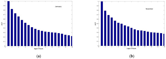
Figure 2. Autocorrelation function of HAWS for (a) January and (b) November.

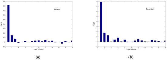
Figure 3. Partial Autocorrelation function of HAWS for (a) January and (b) November.

ACF and PACF are used to determine an adequate group of ARMA models. Appropriate orders $(p,q)$ are determined with the help of an additional criterion, such as Akaike information criterion [Storres].

$$AIC(p,q)=(Y.N)\cdot \ln \left({\sigma }_{\epsilon }^2(p,q)\right)+2T)$$

(7)

where T is the total number of parameters to be estimated.

2.3.2. Parameters Estimation Phase

Once p and q have been identified. The model coefficients ${\phi }_i$ and ${\theta }_i$ along the variance of the residuals ${\sigma }_{\epsilon }^2$ can be estimated. The preliminary estimation is done applying the Yule–Walker relations for ${\phi }_i$, while ${\theta }_i$ values are obtained using Newton–Raphson Algorithm. Final estimation of the parameters using the method of least squares error. Selected models for each month are presented in Table 1.

Note that for the three studied months, it has been found that $ARMA(3,0)$ is the best model (Table 1).

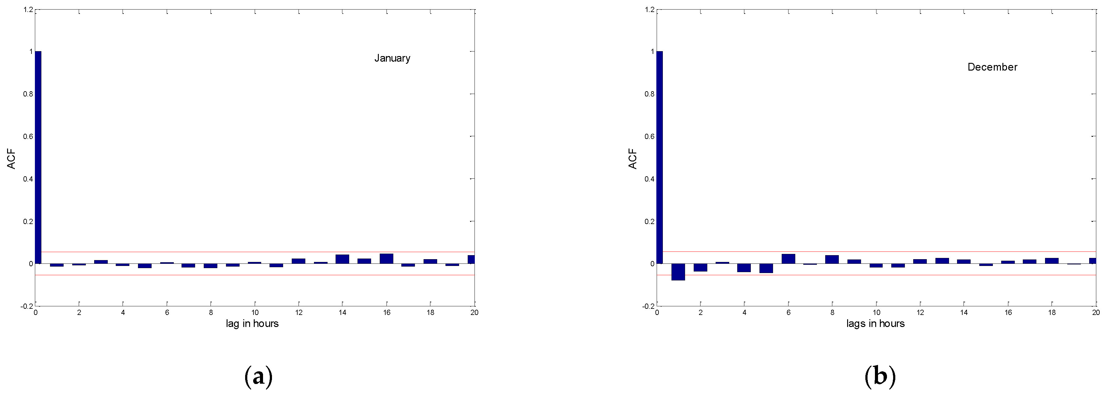
Finally, the models are validated by evaluating the ACF of the residuals. The fitted model can be accepted if the residuals are uncorrelated and normally distributed (Figure 4).

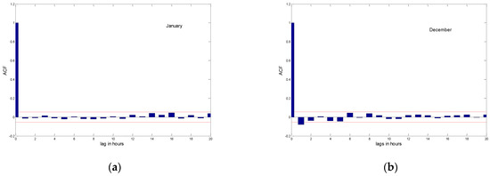
Figure 4. Autocorrelation function of the residues HAWS for (a) January and (b) November.

In order to validate the estimated models, we evaluated the residual autocorrelation functions (Figure 5). If the residuals are jointly independent, their autocorrelation functions cancel for a lag τ = 0. From Figure 5, we can see that the residuals are uncorrelated. Thus the models are retained.

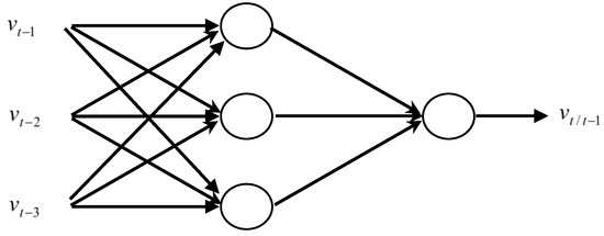
Figure 5. Neural network architecture with four neurons and two layers.

3. The Persistent Model

Persistent model as defined in [5] is given as:

$$v^P{}_{t+h/t}=v_t$$

(8)

Equation (8) is equivalent to saying that the wind at instant h + t is simply the same as it was at time t. This model is developed by meteorologists as a comparison tool to supplement the other models. The accuracy of this model decreases rapidly with an increase of prediction lead time.

4. Neural Networks

Thus far, we have examined linear prediction with ARMA models, which constitute a mostly linear approach to data analysis. Now, we turn to the more complex neural networks. Neural networks have similar uses to linear prediction filters, and can be applied to the same general set of problems.

In general, rules to determine the number of inputs, outputs, and layers do not exist. In the following work, and based on results obtained by Sfetsos (1999) and Erasmo (2009) [9,10], it was decided to use feed-forward ANN (Figure 6). In fact, Sfetsos has found that with the Levenberg–Marquard algorithm as a training method, the feed-forward ANN is very adequate to model the wind speed.

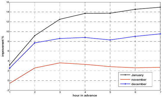
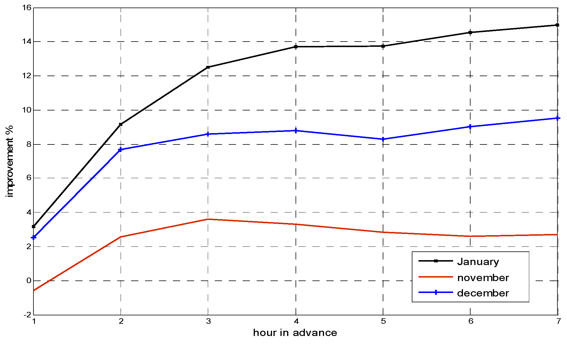
Figure 6. Percentage improvement of RMSE of the ANN forecasts when TS-HAWS are used opposed to HAWS.

The response of the ANN output neuron is:

$$v_t=f_2\left({\displaystyle \sum _{q=1}^3{w}_q{f}_1\left({\displaystyle \sum _{j=1}^3{w}_{q,j}}{v}_{t-j}+bj\right)+b_q}\right)$$

(9)

where $f_1$ and $f_2$ are nonlinear sigmoid activation functions.

The proposed ANN networks are trained to predict the wind speed one step ahead. Prediction of h hours in advance is obtained iteratively, i.e., $v_{t+2/t}^{(ANN)}$ is predicted using $v_{t+1/t}^{(ANN)}$, $v_{t+3/t}^{(ANN)}$ is predicted using $v_{t+3/t}^{(ANN)}$, and so on.

5. Forecast Combination

When several candidate models are available to forecast single variable, we can either select the best model or combine them. Combination of forecast is very advised in case of doubt about the existence of the best model. Our purpose in the following section is to build a linear combination $v_{t/t-h}^{Comb}$ of the competing forecasts as:

$$v_{t/t-h}^{Comb}=w_t^{(ARMA)}{v}_{t/t-h}^{(ARMA)}+w_t^{(ANN)}{v}_{t/t-h}^{(ANN)}$$

(10)

where $w_t^{(ARMA)}$ and $w_t^{(ANN)}$ are time varying coefficients that are updated recursively using recursive least square method (RLS). RLS estimation consists of minimizing the cost function given as:

$$\begin{array}{ll}{S}_t^2(\mathbf{w})& ={{\displaystyle \sum _j^t\kappa (t,j)\left(v_{j/j-h}^{Comb}-\mathbf{w}\cdot {\mathbf{v}}_{j/j-h}^{}\right)}}^2\\ & =S_{t-1}^2(\mathbf{w})+\kappa (t,t){\left(v_{t/t-h}^{Comb}-\mathbf{w}\cdot {\mathbf{v}}_{t/t-h}^{}\right)}^2\end{array}$$

(11)

where $\mathbf{w}=\left[\begin{array}{cc}{w}^{(ARMA)}& w^{(ANN)}\end{array}\right]$, ${\mathbf{v}}_{t/t-h}=\left[\begin{array}{cc}{v}_{t/t-h}^{(ARMA)}& v_{t/t-h}^{(ANN)}\end{array}\right]$ and $\kappa (t,j)$ is the forgetting profile. Usually, $\kappa (t,j)={\Pi }_{i=j+1}^t{\lambda }_i$, where $0\le {\lambda }_i\le 1$ is the forgetting factor [11] The forgetting profile $\kappa (t,j)$ is the weight associated to the jth residual and it allows to reduce the importance of old data recursively.

According to [11], the RLS estimator of ${\mathbf{w}}_{\mathbf{t}}$ is given as:

$${\mathbf{w}}_{\mathbf{t}}={\mathbf{w}}_{\mathbf{t}-\mathbf{1}}+{\mathbf{\Gamma }}_{\mathbf{t}}{\mathbf{v}}_{\mathbf{t}/\mathbf{t}-\mathbf{1}}{a}_t$$

(12)

where $a_t=v_t-{\mathbf{v}}_{\mathbf{t}/\mathbf{t}-\mathbf{1}}{\mathbf{w}}_{\mathbf{t}-\mathbf{1}}$, which is the one step-ahead prediction error, and ${\mathbf{\Gamma }}_{\mathbf{t}}$ is called the gain matrix or the weighted covariance matrix that can be estimated as [12]:

$${\mathbf{\Gamma }}_t=\frac{1}{\lambda }\left({\mathbf{\Gamma }}_{t-1}-\frac{{\mathbf{\Gamma }}_{t-1}{\mathbf{v}}_{\mathbf{t}/\mathbf{t}-\mathbf{1}}{{\mathbf{v}}_{\mathbf{t}/\mathbf{t}-\mathbf{1}}}^{\prime }{\mathbf{\Gamma }}_{t-1}}{\lambda +{{\mathbf{v}}_{\mathbf{t}/\mathbf{t}-\mathbf{1}}}^{\prime }{\mathbf{\Gamma }}_{t-1}{\mathbf{v}}_{\mathbf{t}/\mathbf{t}-\mathbf{1}}}\right)$$

(13)

The choice of $\lambda$ is very important in the recursive estimation of weights. It is indicated in [13] that most applications use a constant forgetting factor typically inside $0.950\le \lambda \le 0.999$.

6. Results and Discussion

To allow a comparison of models, the evolution of the RMSE is evaluated for the persistent, ARMA, feed-forward, and combined models when forecasts are done 1–7 h in advance.

For ANN models, it has been found that forecasting wind speed using TS-HAWS instead of HAWS data yields better performances. As indicated in Table 2, only in one case, forecasting with HAWS has provided lower RMSE (1 h ahead in November). Improvement of forecasting with TS-HAWS over HAWS is presented in Figure 6. Maximum improvement of 15% has been obtained in January when forecasting 7 h ahead.

Table 2. Prediction performances comparison between transformed and non-transformed data.

Hours in Advance	RMSE (January)		RMSE (November)		RMSE (December)
	HAWS	TS-HAWS	HAWS	TS-HAWS	HAWS	TS-HAWS
1	1.2933	1.2522	1.3188	1.3264	1.4032	1.3675
2	1.6143	1.4666	1.6987	1.6551	1.8266	1.6864
3	1.8770	1.6426	1.9715	1.9008	2.1000	1.9197
4	2.0053	1.7306	2.1686	2.0973	2.2858	2.0847
5	2.1302	1.8374	2.2954	2.2302	2.4260	2.2246
6	2.2145	1.8922	2.3655	2.3038	2.5648	2.3334
7	2.2723	1.9322	2.4007	2.3359	2.6599

For all the studied cases, we have found that the RMSE of the persistence models are greater than the RMSE of the other models (Table 3). These results are similar to those obtained by Torres [5] and Sfetsos [6], which indicated that ARMA- and ANN-based models provide better forecasts than the persistence models.

Table 3. Prediction performances for January.

Hour in Advance	RMSE in m/s				Improvement over the Persistent Model %
	Persistent	ARMA	ANN	Combined	ARMA	ANN	Combined
1	1.3676	1.2352	1.2522	1.2347	9.6845	8.4387	9.7188
2	1.7368	1.4546	1.4666	1.4542	16.2518	15.5609	16.2737
3	2.0730	1.6315	1.6426	1.6311	21.2987	20.7610	21.3178
4	2.2489	1.7308	1.7306	1.7310	23.0383	23.0483	23.0303
5	2.4499	1.8341	1.8374	1.8343	25.1331	25.0000	25.1272
6	2.5899	1.8922	1.8922	1.8926	26.9397	26.9372	26.9237
7	2.7073	1.9361	1.9322	1.9368	28.4834	28.6281	28.4596

In 66.67% of the studied cases, it has been found that ARMA models provide relatively lower RMSE than ANN models (Table 3 and Table 4). Evaluation of the forecasting improvement of ARMA models over ANN models varies between −0.61% and 03.49%. These results differ from that obtained by Strores (1999), who has found that ANN models can achieve lower RMSE than ARMA models.

Table 4. Prediction performances for November.

Hour in Advance	RMSE in m/s				Improvement over the Persistent Model (%)
	Persistent	ARMA	ANN	Combined	ARMA	ANN	Combined
1	1.3621	1.3114	1.3264	1.3104	3.7196	2.6187	3.7928
2	1.7986	1.6550	1.6551	1.6494	7.9842	7.9780	8.2972
3	2.1484	1.8999	1.9008	1.8949	11.5639	11.5260	11.7971
4	2.4454	2.0983	2.0973	2.0912	14.1958	14.2358	14.4833
5	2.6646	2.2245	2.2302	2.2184	16.5186	16.3015	16.7471
6	2.8103	2.2948	2.3038	2.2888	18.3407	18.0203	18.5543
7	2.8887	2.3252	2.3359	2.3179	19.5068	19.1383	19.7606

Combined models provide relatively better performances than the ARMA and the ANN models a few hours in advance (1–4 h); however, for long-term forecasting, individual models can provide lower RMSE than the combined models (Table 3).

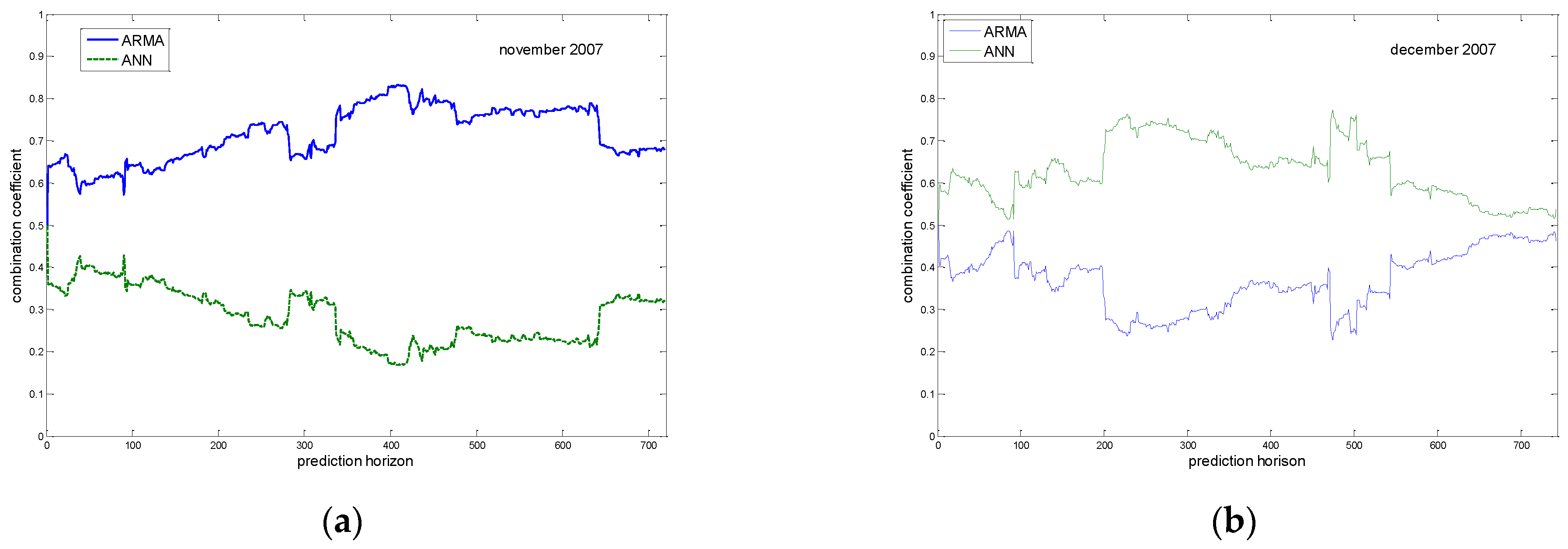
To better understand the role of individual models in the final combination, we have presented in Figure 7 the variation of the combination coefficients when real wind is measured for November and December 2007. The first 100 wind speed values have been used to initialize coefficients and the covariance matrix. Figure 7a shows that the coefficient of the ARMA model is greater than the one of the ANN model, which means that the ARMA model is providing lower error for November 2007. In December 2007, and as indicated in Figure 7b, the ANN model forecasts the wind speed better than ARMA models.

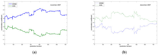
Figure 7. Evolution of the combination coefficient for November and December.

7. Conclusions

In this study, models based on ARMA methodology as well as ANN theory have been proposed to forecast the hourly wind speed. The obtained results have indicated that both ARMA and ANN models are capable to predict wind speed for few hours in advance. Performances comparison between ARMA and ANN models has indicated that their performances are very close.

An adaptive combination of the two proposed approaches has proposed to improve the forecasting performances. The obtained results have indicated that for a few hours in advance, the combined model outperform the individual models.

For ANN modeling, it has been found in this work that the use of the transformed and standardized TS-HAWS provides better results than HAWS.

References

- Geerts, H.M. Short range prediction of wind speeds: A system-theoretic approach. In Proceedings of the European Wind Energy Conference, Hamburg, Germany, 22–26 October 1984; pp. 594–599. [Google Scholar]
- Daniel, A.; Chen, A. Stochastic simulation and forecasting of hourly average wind speed sequence in Jamaica. Sol. Energy 1991, 46, 1–11. [Google Scholar] [CrossRef]
- Nfaoui, H.; Essiarab, H.; Sayigh, A.H. A stochastic Markov chain model for simulating wind speed time series at Tangiers, Morocco. Renew. Energy 2004, 29, 1407–1418. [Google Scholar] [CrossRef]
- Kamal, L.; Jafri, Y.Z. Time series models to simulation and forecast hourly averaging wind speed in Quetta, Pakistan. Sol. Energy 1997, 61, 23–32. [Google Scholar] [CrossRef]
- Torres, J.; Garcia, A.; De Blas, M.; De Francisco, A. Forecast of hourly averaged wind speed with ARMA models in Navarre (Spain). Sol. Energy 2005, 79, 65–77. [Google Scholar] [CrossRef]
- Sfetsos, A. A comparision of various forecasting techniques applied to mean hourly wind speed time series. Renew. Energy 2000, 21, 23–35. [Google Scholar] [CrossRef]
- More, A.; Deo, M. Forecasting wind with neural networks. Mar. Struct. 2003, 16, 35–49. [Google Scholar] [CrossRef]
- Erasmo, C.; Wilfrido, R. Wind speed forecasting in the South Coast of Oaxaca, México. Renew. Energy 2007, 32, 2116–2128. [Google Scholar]
- Sfetsos, A. A novel approach for the forecasting of mean hourly wind speed time series. Renew. Energy 2002, 27, 163–174. [Google Scholar] [CrossRef]
- Erasmo, C.; Wilfrido, R. Short term wind speed forecasting in la Venta, Oaxaca, México, using artificial networks. Renew. Energy 2009, 34, 274–278. [Google Scholar]
- Sanchez, I. Adaptive combination of forecasts with application to wind energy. Int. J. Forecast. 2008, 24, 679–693. [Google Scholar] [CrossRef]
- Grillenzoni, C. Optimal recursive estimation of dynamic models. J. Am. Stat. Assoc. 1994, 89, 777–787. [Google Scholar] [CrossRef]
- Sanchez, I. Short-term prediction of wind energy production. Int. J. Forecast. 2006, 22, 43–65. [Google Scholar] [CrossRef]
Disclaimer/Publisher’s Note: The statements, opinions and data contained in all publications are solely those of the individual author(s) and contributor(s) and not of MDPI and/or the editor(s). MDPI and/or the editor(s) disclaim responsibility for any injury to people or property resulting from any ideas, methods, instructions or products referred to in the content. |
© 2023 by the author. Licensee MDPI, Basel, Switzerland. This article is an open access article distributed under the terms and conditions of the Creative Commons Attribution (CC BY) license (https://creativecommons.org/licenses/by/4.0/).