Reliability of Strength Test Results on Materials Using Statistical and Computational Methods ^†

Abstract

Destructive testing evaluates material strength but prohibits repeated measurements on the same specimen. Finite element simulations, such as those using ANSYS Mechanical, provide a cost-effective alternative by delivering deterministic solutions under defined conditions. To incorporate input variability, the Monte Carlo method applies assigned probability distributions to parameters like magnitude and angle of the applied force and geometric tolerances of the specimen. Thus, input variability yields distributions for output such as stress and deformation, enabling uncertainty quantification. In this study, an example of static force on a concrete cube was modeled in ANSYS, and uncertainty was propagated using the Monte Carlo method, as described in JCGM 101:2008. This approach enables the identification of critical factors affecting the outcome and provides confidence intervals that might be used as decision rules to support comparisons of numerical simulations with experimental data and of results of different models and to calculate the limits of quality control charts of a testing laboratory.

1. Introduction

ANSYS, a commercially available finite element software, can simulate ordinary concrete’s mechanical properties, and it is used to analyze concrete elements [1]. It enables engineers to model the mechanical behavior of concrete and other materials at a very fine level of detail. The simulation process in ANSYS involves modeling the concrete structure as a three-dimensional (3D) network of interconnected finite elements. Loads are then applied to the model to simulate the mechanical behavior of the concrete, taking into account the material properties. The finite element method (FEM) is a method widely used for calculation of structural properties, stresses, strains, and deformations of structures. The rapid and continuous advancement in computational power has significantly expanded the scope and scale of numerical simulation techniques, enabling the analysis of increasingly complex physical systems with higher efficiency and resolution and potentially greater accuracy depending on the underlying models.

The uncertainty in a system can be present in multiple aspects, such as loading conditions or geometric and material properties. The deterministic approach assumes exact, fixed values for inputs like material properties, boundary conditions, and loading. On the other hand, the probabilistic approach [2,3] is a method used to account for uncertainty and variability in input data, model parameters, or environmental conditions when analyzing or designing systems. Instead of assuming that all parameters are fixed (as in a deterministic approach), the probabilistic approach treats key inputs as random variables with known or definable probability distributions. These distributions can assume any mathematically definable form. A common example is the normal (or Gaussian) distribution. This approach allows for the prediction not just of a single outcome, but a range of possible outcomes, each with a quantifiable likelihood [4]. By integrating the probabilistic approach into finite element analysis, the simulation is transformed from a single-point deterministic prediction into a statistical evaluation of the likelihood of various outcomes. This is typically achieved through techniques such as the Monte Carlo method [5,6,7], in which the model is executed repeatedly using input parameters that are randomly sampled from predefined probability distributions. This process results in a range of possible outputs rather than a single solution, allowing for the assessment of variability, the identification of influential parameters, and the quantification of uncertainty in the system’s response. Figure 1 illustrates the propagation of distributions for N = 3 independent input quantities.

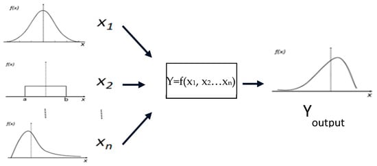
Figure 1. Schematic view of Monte Carlo simulation for propagating distributions (e.g., to estimate measurement uncertainty).

JCGM 101:2008 [8], titled “Evaluation of Measurement Data—Supplement 1 to the ‘Guide to the Expression of Uncertainty in Measurement’—Propagation of Distributions Using a Monte Carlo Method”, is an internationally recognized document published by the Joint Committee for Guides in Metrology (JCGM). Generally, it provides comprehensive guidance on how to evaluate and propagate uncertainty when the input quantities of a measurement or computational model are represented by probability distributions. This supplement promotes the use of the Monte Carlo method as a practical and powerful tool for numerically simulating the propagation of uncertainty through complex models.

When engineers use the results of a simulation, their goal is often to compare the outcome either to an experimental result or to another computational model outcome. In both cases, understanding and quantifying the uncertainty associated with the simulation is crucial. If a simulation is to be compared with an experiment, it is not feasible to simply match the mean or nominal values; a decision rule needs to be selected. Without accounting for this, any apparent decision on agreement or disagreement could be misleading. Uncertainty intervals provide context for whether the results are statistically consistent or significantly different. Without uncertainty quantification, simulation–experiment comparisons lack scientific rigor. Similarly, when comparing two different models, each with its own assumptions, simplifications, and input data, uncertainty quantification allows engineers to determine whether the models produce results that are meaningfully distinct or within acceptable agreement. This is particularly important for model validation, quality control, or selecting a model for use in a safety-critical or high-precision application.

In this study, a simple finite element model of a concrete cube was developed in ANSYS 2025 R2 to simulate the mechanical response under load. Recognizing that real-world variability—such as geometric tolerances of the specimen or variability in the magnitude and misalignments of applied forces—can significantly affect test outcomes, these input parameters were modeled as random variables with assigned probability distributions. To propagate this uncertainty through the model and obtain distributions of output quantities (such as maximum deformation, strain, and stress), the Monte Carlo method was employed in the way that is explicitly proposed by JCGM 101:2008.

In destructive testing, estimating the uncertainty of the measurement is typically achieved through repeated tests on multiple specimens. However, this approach inevitably introduces the effect of material heterogeneity, as each specimen may differ in composition, geometry, or internal structure. This variation can obscure the influence of specific factors on the test outcome. By assigning probability distributions to input parameters, it becomes possible to evaluate their individual and combined effects on the output without the confounding influence of specimen-to-specimen variability. Beyond identifying which factors contribute most to the result, this method enables the calculation of confidence intervals for key mechanical quantities. These intervals can be used as the basis for decision-making, including comparing simulation outcomes with experimental data from a single physical specimen, assessing the consistency between two different models, and defining control limits for quality assurance in laboratory testing procedures. In this way, the Monte Carlo-based approach, as introduced in JCGM 101:2008, provides a more robust alternative [5,6,7,8,9]. Not only does it quantify uncertainty in a traceable and standardized manner, but it also enhances the interpretability and applicability of simulation results in engineering practice.

In a previous study [10], a methodology was presented for combining the results of compressive strength testing of concrete specimens with two non-destructive testing methods, providing additional results on strength determination based on totally different measurement mechanisms. The approach developed in the present work aims to further enhance the reliability of the destructive testing method. By incorporating numerical simulations and uncertainty quantification through Monte Carlo analysis, this method provides deeper insight into the variability and sensitivity of key parameters affecting the outcome of compressive strength tests. As a result, it strengthens the interpretive value of destructive tests by complementing their single-value results with a probabilistic framework. This integration supports more robust conformity assessments and contributes to improving the overall quality control procedures in accordance with modern standards.

The significance of this study is that (i) it presents a method for obtaining a decision rule when comparing the model results with the results of an experiment on the real specimen or when comparing the results of two different models, and (ii) it proposes a method to enhance the reliability of destructive testing. The uncertainty quantification is essential to engineers who want to validate any model.

2. Method—Input Parameters and Randomization Procedure

A simple example of FEM application (a 3D model of a concrete cube with dimensions 150 × 150 × 150 mm) was chosen for the determination of maximum total deformation, maximum principal elastic strain, and maximum principal stress. It should be noted that this introduces an ideal, perfectly shaped specimen that is impossible to manufacture in the real world. Figure 2a shows one side of this specimen where the deviations from the ideal cube are emphasized enough to be visible. In this figure, the red line represents a cross section of the real surface of the specimen, the blue line is the same cross section but for a perfectly flat and perpendicular side of the specimen that could be considered as representative of the real side on average, and the gray line is the cross section of the perfectly flat and perpendicular side in the plane at the nominal (150 mm) dimension of the specimen. Correspondingly, the same figure introduces many significant errors produced by the model deviations: a. lack of perpendicularity of the surface, shown as angle θ of the real side (red line) relative to the plane where the representative and the nominal sides are lying; b. roughness of the surface (non-linearity of the red line); and c. offset of the average plane of the specimen side (blue line) relative to the nominal plane of the specimen (gray line). These occur naturally and are expectedly due to imperfections in the construction of the molds and deviations in the molding or specimen curing process.

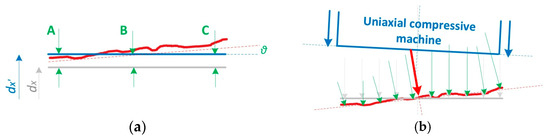
Figure 2. (a) Effect of lack of flatness and perpendicularity of the specimen side on the evaluation of the specimen dimensions (example on evaluating the dimension of the specimen parallel to the x-axis). Τhe red line represents a cross-section of the real surface of the specimen. (b) Imperfections in Load Application: Schematic showing the effects of non-perpendicularity in the moving platen of the uniaxial compression machine and non-flatness of the specimen’s upper face.

When attempting to evaluate the real characteristics of a cube specimen, it is natural to measure the dimensions of each side, e.g., by using a properly calibrated caliper. As shown in Figure 2a, a good approach is to make at least three measurements, one in the middle and two more near the extremities of each side of the specimen (i.e., points shown by the green arrows in the case of the side parallel to axis x). This way, a mean (variable d_x′) of the side dimension and a scale of dispersion, in the form of a calculated standard deviation s_dx′, are obtained. A correct representation of this side dimension is a confidence interval assuming a normal (Gaussian) distribution of variable d_x′, at a 95% level, should be referred to as d_x′ ± 1.96·s_dx′. Of course, this interval is biased when compared to the nominal (i.e., the desired) value, with a corresponding systematic error equal to d_x − d_x′.

One side of the cube was chosen as fixed, and a force, nominally chosen to be equal to F, was applied perpendicular to the opposite side. Figure 2b shows how the lack of flatness of the surface of the specimen, but also the lack of alignment with the moving part of a uniaxial compressive machine, affects the vector of the applied force. The nominal testing condition corresponds to a totally perpendicular compressive force, equal to F, evenly distributed through the entire side of the specimen. Again, the real test conditions deviate from this, producing many significant errors: (a) error in defining the scale of the applied force, which is expected even for successfully calibrated uniaxial compressive machines, and (b) error due to deviation from the desired situation of perfectly flat specimen surface and perfectly aligned axis of the moving part of the compressive machine relative to the perpendicular axis of the specimen.

Parameters P1–P3 represent the three Cartesian dimensions (d_x, d_y, d_z) of the cube (Figure 3b), specified nominally as 150 mm. While molds are designed for these nominal values, manufacturing tolerances and surface irregularities result in deviations. The actual dimensions (d_x′, d_y′, d_z′) are best represented as a mean ± standard deviation, assuming a normal distribution. In practice, up to 10 caliper measurements per specimen provide a small but sufficient dataset for estimating these values.

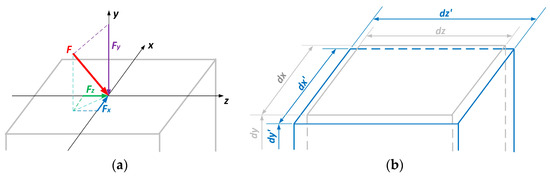
Figure 3. Definition of input parameters: (a) force vector F, defined by its magnitude and angle relative to the horizontal, with Cartesian components P4–P6 referenced from the specimen’s top-face center. (b) Dimensions of the cube specimen (parameters P1–P3): nominal values (d_x, d_y, d_z = 150 mm) and measured values (d_x′, d_y′, d_z′), which vary due to manufacturing tolerances.

Parameters P4–P6 denote the Cartesian components of the applied force F, which is the resultant force due to the compression of the upper surface of the specimen, referenced from the center of the specimen’s upper face (Figure 3a). Although the intended loading is perpendicular to this face, imperfections in machine alignment and specimen flatness (Figure 2b) introduce small components along the horizontal axes. Calibration data provide the mean and standard deviation for the vertical component, while the horizontal components are estimated from reasonable engineering assumptions.

Random numbers were generated in Microsoft Excel using the formula =NORM.INV(RAND(), m, sd), where RAND() produces a uniformly distributed value between 0 and 1, and NORM.INV converts it into a normally distributed variate with specified mean (m) and standard deviation (sd). Large sets of values for each input parameter (P1–P6) were generated according to selected means and standard deviations. Values for input parameter P6 were not generated directly using the randomization function. It was decided that the randomization function should be applied for parameter F, which is originally correlated with the setup of the compressive machine. The force components on the x and z axes are due to the lack of flatness of the upper surface of the specimen and of its alignment with the moving part of the compressive machine. The component of force F_z on the perpendicular axis z, the parameter P6, was then calculated as (Figure 3a):

$$F_y = \sqrt{F^2-F_x^2-F_z^2}.$$

(1)

To validate Excel’s random number generation, the simulated datasets were subjected to normality testing (Table 1).

Table 1. Normality test on the set of values produced by the randomization algorithms.

Input Parameters	n	Mean	Standard Deviation	Median	Normality Test Statistics (& Result *)			Skewness	Kurtosis
					W/S-W	D/K-S	A2/A-D
P1	5000	149.9797	0.5209	149.9735	0.9996 (succ. *)	0.0099 (succ.)	0.5501 (succ.)	0.0260	−0.0096
P2	5000	150.8522	0.8199	150.8483	0.9998 (succ.)	0.0087 (succ.)	0.1856 (succ.)	0.0049	0.0702
P3	5000	150.0633	0.4826	150.0662	0.9998 (succ.)	0.0060 (succ.)	0.1522 (succ.)	−0.0056	0.0134
P4	5000	10,004.8073	2.7119	10,004.8179	0.9994 (succ.)	0.0069 (succ.)	0.2428 (succ.)	−0.0086	0.1560
P5	5000	45.6836	23.1312	45.5944	0.9995 (succ.)	0.0089 (succ.)	0.3593 (succ.)	0.0324	0.1098
P6	5000	65.3273	30.0306	65.5343	0.9997 (succ.)	0.0070 (succ.)	0.2727 (succ.)	0.0412	−0.0182

* succ. = successful normality test, which means compliance with normal distribution.

For each dataset, the first 5000 values were tested to verify consistency with a normal distribution, using the Shapiro–Wilk (S–W), Kolmogorov–Smirnov (K–S), and Anderson–Darling (A–D) tests. The S–W test, recommended for small to moderate samples (n ≈ 3–5000), compares ordered sample values with expected normal order statistics, with W values near 1 indicating normality. At the upper range (n = 5000), results were corroborated by the K–S test, which compares the empirical and theoretical cumulative distribution functions, using the maximum vertical distance (D) as the test statistic. To match the study population (n = 404), the first 404 values from each dataset were also tested. At this sample size, both S–W and K–S tests are appropriate, with the former generally more sensitive to deviations in symmetric distributions. The A–D test, a modification of the K–S procedure, emphasizes deviations in the distribution tails, with its statistic (A²) measuring the integrated squared difference between empirical and theoretical distributions, providing greater power for detecting outliers and extreme-value departures from normality across all sample sizes.

3. Results

The method was used to determine the distribution of the output parameters based on repeats of the model solution using the first 404 generated sets of randomized values. The output parameter data were obtained in the form of a set of 404 values for each. As a result, each one of the three output parameter distributions (P7, P8, P9) was turned into a histogram, thus providing the exact range and shape of the output distribution (Figure 4). Figure 4 illustrates a probabilistic analysis workflow where input distributions of geometric dimensions and force components are propagated through a computational model, resulting in output distributions. This figure is similar to Figure 1, but the presenting distributions are made by the exact results of the applied method. The three histograms obtained for output parameters represent the distributions of response quantities obtained from the model. The statistical characteristics of the resulting distributions are presented in detail in Table 2.

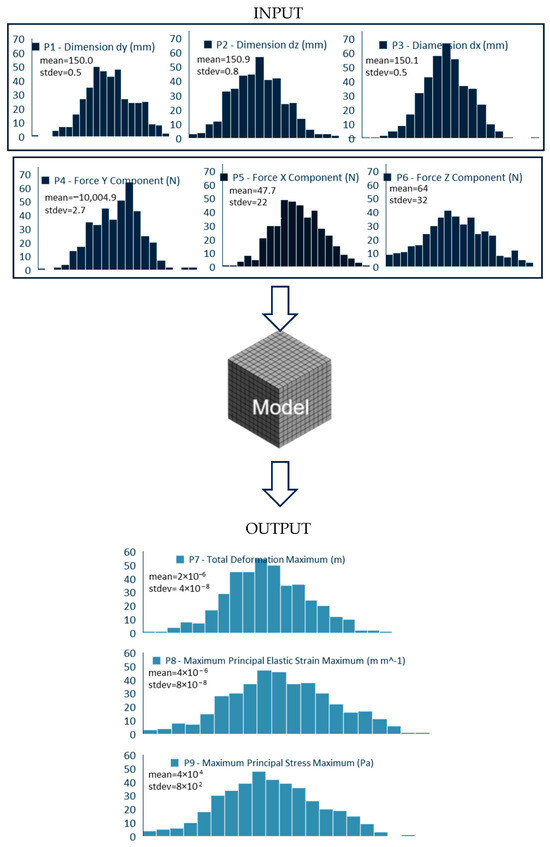
Figure 4. Distributions of input and output parameters.

Table 2. Normality test on the input dataset and on the results of the Monte Carlo propagation.

Input Parameters	n	Mean	Standard Deviation	Median	Normality Test Statistics (& Result *)			Skewness	Kurtosis
					W/S-W	D/K-S	A2/A-D
P1	404	150.0013	0.5442	149.9731	0.9944 (succ. *)	0.0363 (succ.)	0.6855 (succ.)	0.0333	−0.2065
P2	404	150.9182	0.8159	150.8937	0.9955 (succ.)	0.0261 (succ.)	0.2742 (succ.)	0.2453	0.1212
P3	404	150.0921	0.4790	150.0904	0.9954 (succ.)	0.0405 (succ.)	0.4217 (succ.)	−0.0278	0.5277
P4	404	10,004.9420	2.7301	10,004.7700	0.9940 (succ.)	0.0462 (succ.)	0.7319 (succ.)	0.0217	0.1443
P5	404	47.6749	22.4098	46.8054	0.9980 (succ.)	0.0290 (succ.)	0.2894 (succ.)	0.0389	−0.1867
P6	404	63.9890	31.6542	62.7139	0.9933 (succ.)	0.0219 (succ.)	0.2897 (succ.)	0.0472	−0.4270
P7	404	2.3186·10−6	3.8393·10−8	2.3165·10−6	0.9916 (failed)	0.0799 (failed)	1.5705 (failed)	0.1152	0.0609
P8	404	4.0387·10−6	7.9600·10−8	4.0342·10−6	0.9946 (succ.)	0.0532 (succ.)	0.6267 (succ.)	0.0478	−0.2581
P9	404	35,605.9099	762.7816	35,554.0313	0.9963 (succ.)	0.0315 (succ.)	0.3688 (succ.)	0.0567	−0.2572

* succ. = successful normality test, which means compliance with normal distribution.

Initially, the output parameters’ values were tested against the normal distribution (Table 2). The normality test succeeded for parameters P8 and P9, meaning that values equal to m ± 1.96·sd correspond to a 95% confidence interval. For P8, the 95% confidence interval is (4.0 ± 0.2) ×10⁻⁶ mm^−1, and for P9 it is (3.6 ± 0.1) ×10⁴ Pa. These two intervals may be used in a decision rule for comparison with specified limits. Another use of them is to compare the values produced from two different simulations for two different, but similar, specimens.

The normality test was not successful for the distribution of values for the output parameter P7. Following an attempt to test whether this distribution complies with the t-distribution, which is also a symmetrical, centralized distribution like the normal distribution. A chi² test was performed, leading to the conclusion that the parameter P7 data does not comply with the t-distribution.

This process could be followed for other known symmetrical distributions until a chi² test reveals the real distribution for the values of the output parameter P7. Nevertheless, assigning a triangular distribution in this case of a symmetrical and centralized outcome for parameter P7 (Figure 4) would be adequate to proceed with establishing a decision rule.

The method analyzed in this study is presented in a way that it could be utilized in any finite element solution of a material’s strength problem to produce a criterion for experimental results verification, based on the 95% estimated confidence interval for the strength result.

The confidence intervals estimated based on the methodology presented for the model results through the Monte Carlo method can be used:

• As the basis for a decision rule when comparing the model results with the results of an experiment on the real specimen.
• As the basis for a decision rule when comparing the results of two different models.
• To calculate the limits of quality control charts of a laboratory performing the testing.

4. Conclusions

Even in cases of destructive tests where the results cannot be repeated, the presented method can offer an opportunity for analyzing the uncertainty of these results based on estimations for the distribution of the influencing parameters.

References

- Gowram, I.; Beulah, M.; Mohamed, M.M.I.; Ibrahim, S.A.M.; Puneeth, V.; Moussa, S.B.; Nasr, S. Experimental and finite element studies on the mechanical properties of high-strength concrete using natural zeolite and additives. Alex. Eng. J. 2024, 109, 989–993. [Google Scholar] [CrossRef]
- de Lima, B.S.L.P.; Ebecken, N.F.F. A comparison of models for uncertainty analysis by the finite element method. Finite Elem. Anal. Des. 2000, 34, 211–232. [Google Scholar] [CrossRef]
- Mangado, N.; Piella, G.; Noailly, J.; Pons-Prats, J.; Ballester, G.M.A. Analysis of Uncertainty and Variability in Finite Element Computational Models for Biomedical Engineering: Characterization and Propagation. Front. Bioeng. Biotechnol. 2016, 4, 85. [Google Scholar] [CrossRef] [PubMed]
- Dar, F.H.; Meakin, J.R.; Aspden, R.M. Statistical methods in finite element analysis. J. Biomech. 2002, 35, 1155–1161. [Google Scholar] [CrossRef] [PubMed]
- Theodorou, D.; Meligotsidou, L.; Karavoltsos, S.; Burnetas, A.; Dassenakis, M.; Scoullos, M. Comparison of ISO-GUM and Monte Carlo methods for the evaluation of measurement uncertainty: Application to direct cadmium measurement in water by GFAAS. Talanta 2011, 83, 1568–1574. [Google Scholar] [CrossRef] [PubMed]
- Mahmoud, G.M.; Hegazy, H. Comparison of the GUM and Monte Carlo methods for uncertainty estimation in complex measurement problems. Int. J. Metrol. Qual. Eng. 2017, 8, 10. [Google Scholar]
- Zhang, J. Modern Monte Carlo methods for efficient uncertainty quantification and propagation: A survey. Wiley Interdiscip. Rev. Comput. Stat. 2019, 11, e1463. [Google Scholar] [CrossRef]
- Joint Committee for Guides in Metrology (JCGM). Evaluation of Measurement Data—Supplement 1 to the “Guide to the Expression of Uncertainty in Measurement”—Propagation of Distributions Using a Monte Carlo Method (JCGM 101:2008); Bureau International des Poids et Mesures: Sèvres, France, 2008. [Google Scholar]
- Widmaier, T.; Hemming, B.; Juhanko, J.; Kuosmanen, P.; Esala, V.-P.; Lassila, A.; Laukkanen, P.; Haikio, J. Application of Monte Carlo simulation for estimation of uncertainty of four-point roundness measurements of rolls. Precis. Eng. 2017, 48, 181–190. [Google Scholar] [CrossRef]
- Gavela, S.; Karydis, G.; Papadakos, G.; Zois, G.; Sotiropoulou, A. Uncertainty of concrete compressive strength determination by a combination of Rebound Number, UPV and uniaxial compressive tests on cubical concrete samples. Mater. Today Proc. 2023, 93, 641–645. [Google Scholar] [CrossRef]
Disclaimer/Publisher’s Note: The statements, opinions and data contained in all publications are solely those of the individual author(s) and contributor(s) and not of MDPI and/or the editor(s). MDPI and/or the editor(s) disclaim responsibility for any injury to people or property resulting from any ideas, methods, instructions or products referred to in the content. |
© 2025 by the authors. Licensee MDPI, Basel, Switzerland. This article is an open access article distributed under the terms and conditions of the Creative Commons Attribution (CC BY) license (https://creativecommons.org/licenses/by/4.0/).