Localization of Unknown Nodes on UWSN Using the Linear Constraint Optimization Technique Based on Energy and Distance (LUCOTED) ^†

Abstract

Underwater Wireless Sensor Networks (UWSNs) are widely used technologies in aquatic environments. However, these types of networks face several constraints caused by the mobility of nodes, energy consumption, and constraints due to acoustic communication. In light of this, the location of nodes appears as a promising axis for improving the services expected from these networks. To address these, we suggest the LUCOTED approach—a Linear Constraint Optimization Technique for estimating unknown node positions by selecting anchor nodes with the highest energy and shortest distance, based on randomly initialized conditions. It achieves 98% accuracy, exceeding Gradient Descent and Trilateration methods. Moreover, our method LUCOTED outperforms the DEEC algorithm in terms of error when the number of anchor nodes is below 80 and achieves higher accuracy than the EPRP technique when the number exceeds 100.

1. Introduction

The 2023 UNFCCC Ocean Dialogue demonstrated the significant impacts of aquatic ecosystems on human health as well as the potential of aquatic foods as climate solutions. Also, the State of World Fisheries and Aquaculture (SOFIA) 2024 edition [1] reports that worldwide fisheries and aquaculture production increased by 4.4 percent from 2020 to 223.2 million tons in 2022. Since 57% of the world’s population relies on aquaculture for food, the oceans also support international maritime transportation, preserve marine biodiversity, and maintain climatic balance This rich area needs a promising technology for collecting, processing, sharing, and transmitting data from aquatic locations to land-based stations, like the wireless network of underwater sensors (UWSNs) that enables effective and sustainable activities in hostile environments [2], as shown in Figure 1 [3]. Also, locating nodes, positions, and naming the information gathered are two common uses for location information in UWSN data transfer protocols [4].

Figure 1. UWSN Architecture [3].

On unknown node localization, in three-dimensional space, we use three or more anchor nodes defined by known coordinates, and their distances, respectively, to the unknown node are measured by means of specific methods like Time of Arrival (TOA) [5], Time Difference of Arrival (TDOA) [6], Angle of Arrival (AOA) [7], or Received Signal Strength Indication (RSSI) [8]. Those are four common measurement methods used. Generally, like various approaches in the same context, the trilateration positioning method in UWSN scenes uses anchor node coordinates for unknown node position determination, but positioning error increases due to environmental interference, uncertainty, and other unfavorable circumstances [9]. Low transmission cost, high coverage, localization accuracy, reduced computing costs, enhanced scalability, etc., are the fundamental objectives of localization techniques [10,11], but in our study, the convergence of the algorithm, location error, and energy consumption were the main topics.

The rest of the paper will be structured as follows: Section 2 presents the key factors and restrictions of localizing an unknown node on the UWSN, while Section 3 discusses related works that were established in the same context. We outline the study methodology in Section 4, which consists of setting up algorithms for the localization of unknown nodes. In Section 5, we describe simulation implementation and results. Finally, Section 6 illustrates the conclusion of the research.

2. Localization of Unknown Node’s Factors and Constraints

2.1. Localization Process

The process of locating nodes can be seen as a system formed by three components:

2.1.1. Distance/Angle Estimation

This part is in charge of estimating information concerning the angles and/or distances between two nodes. The received signal strength indicator (RSSI), time [difference] of arrival (ToA/TDoA), number of hops, or angle of arrival (AoA) are known to be methods employed for this component.

2.1.2. Position Computation

This component has the role of determining a node’s location using the information that is currently available regarding the locations and distances/angles of reference nodes.

2.1.3. Localization Algorithm

It establishes how to adapt the information that is currently accessible in order to ensure that the majority of the WSN’s nodes can estimate their positions. It is a distributed algorithm that typically uses multiple hops. Among the most popular algorithms are Directed Position Estimation (DPE) [4] and the Ad Hoc Positioning System (APS) [12]. Add to the localization problem: security will be more critical in the case of the UWSN due to the deployment environment [13].

UWSNs have several applications, like mine detection, disaster prevention, and marine research. However, node localization is limited by underwater environment characteristics like signal attenuation and acoustic properties, making GPS acquisition challenging [14].

2.2. Main Challenges and Constraints

• ▪ Node mobility [15].
• ▪ Time synchronization between nodes [16].
• ▪ Low bandwidth in acoustic communication [17,18].
• ▪ Sound speed variation [19].
• ▪ Energy limitation [20].
• ▪ Security attacks on underwater localization [14,21].

3. Related Works

Several studies on node localization in Underwater Wireless Sensor Networks (UWSNs) confirm that addressing localization challenges improves understanding and management of critical situations. In fact, the research [22] reviews Range-Based and Range-Free localization algorithms, evaluating trade-offs and suggesting enhancements based on a comparative analysis considering coverage area, node density, energy consumption, localization inaccuracy, and computational complexity. The findings guide researchers in selecting or refining optimal localization methods for UWSNs. Authors in [23] summarize existing underwater wireless sensor network (UWSN) localization algorithms as distributed, scalable, and iterative, but these rely heavily on acknowledgment messages for location identification. This research proposes a new Location Finding and Correcting Algorithm (LCLI) aiming to minimize message volume and enhance transmission efficiency. The LCLI efficiently locates nodes while addressing localization errors, and a correction algorithm for additional errors is also introduced. Comparisons show that UWSN-LCLI significantly outperforms existing algorithms. Moreover in [24], the authors classify localization algorithms in UWSNs into stationary, mobile, and hybrid categories, dividing them into centralized and distributed subcategories. They evaluate these algorithms based on anchor type, synchronization time, coverage, accuracy, and computational complexity. Also, in [25] the contributors, analyze UWSN localization approaches using centralized and distributed categories, focusing on error, time, and communication metrics, and describe the techniques used for localizing unknown nodes. In addition, the study [9] introduces a new trilateration algorithm using K-means combination and clustering, proving to minimize mean distance error and improve positioning accuracy compared to the greatest likelihood, least-squares approach, and standard trilateration. Furthermore, in paper [26] authors confirm the effectiveness of their proposed methods, innovative semi-definite programming (SDP), and underwater solvers in enhancing RSS-based localization accuracy. They transform the optimization issue into a convex SDP problem using semi-definite relaxation, offering an advantage over iterative solvers. Equally, work [27] proposes a novel trilateration algorithm for indoor localization using received signal strength indication (RSSI). It uses a Gaussian filter, LSCF technique for transmit power estimation, and a nonlinear error function based on distances and anchor node positions. Similarly, the authors present in [28] “ITL-MEPOS,” an algorithm-based sliding window optimization for the trilateration localization technique. They use SDS-TWR for distance estimation, achieving high accuracy compared to other methods in the same context. In another study [29], Zhou et al. developed a new localization algorithm using AdaDelta Gradient Descent to prevent collaborative attacks on underwater networks. The algorithm improves localization accuracy by iteratively removing falsified data from interfering nodes, ensuring consistent service. Finaly, research [30] shows that a localization model with a hop loss function and anchor nodes improves location accuracy by 86.11% in a randomly distributed network, surpassing the DEM-DV-Hop approach by 6.05%. The contributions of the DEMN and the hop loss are 2.46% and 3.41%, respectively.

4. Methodology of Research

4.1. Mathematical Approach

4.1.1. Objective Function and Constraints

We consider the localization of the unknown node process as a linear optimization problem with constraints, aiming to minimize the objective function by minimizing the error between nodes’ estimated and calculated positions while obeying the following requirements:

• Distance between nodes must be shorter than the range of communication;
• Each node (x, y, z) must be in an area defined by (x_max, y_max, z_max) as 3D dimensions;
• Anchor nodes chosen for localization should both present the highest residual energy and the nearest distance to the unknown node.

Assume that, we have N anchor nodes A[i]: (A[i].x, A[i].y, A[i].z) for i = 1 to N and an unknown node Un: (Un.x, Un.y, Un.z), defined as coordinates of 3D vectors.

We define the objective function as follows:

$$f\left(x,y,z\right)={\mathrm{e}\mathrm{s}\mathrm{t}\mathrm{i}\mathrm{m}\mathrm{a}\mathrm{t}\mathrm{e}}_{\mathrm{d}\mathrm{i}\mathrm{s}\mathrm{t}\mathrm{a}\mathrm{n}\mathrm{c}\mathrm{e}}-{\mathrm{m}\mathrm{e}\mathrm{a}\mathrm{s}\mathrm{u}\mathrm{r}\mathrm{e}}_{\mathrm{d}\mathrm{i}\mathrm{s}\mathrm{t}\mathrm{a}\mathrm{n}\mathrm{c}\mathrm{e}}$$

(1)

$$\mathrm{e}\mathrm{s}\mathrm{t}\mathrm{i}\mathrm{m}\mathrm{a}\mathrm{t}\mathrm{e}{\mathrm{d}}_{\_}\mathrm{d}\mathrm{i}\mathrm{s}\mathrm{t}\mathrm{a}\mathrm{n}\mathrm{c}\mathrm{e}=\sum _{n=1}^{N}d\left(\mathrm{A}\left[\mathrm{i}\right],\mathrm{U}\mathrm{n}\right)$$

(2a)

where $\mathrm{d}\left(\mathrm{A}\left[\mathrm{i}\right],\mathrm{U}\mathrm{n}\right)=\sqrt{\begin{array}{c}{\left(\mathrm{A}\left[\mathrm{i}\right].\mathrm{x}-\mathrm{U}\mathrm{n}.\mathrm{x}\right)}^2+{\left(\mathrm{A}\left[\mathrm{i}\right].\mathrm{y}-\mathrm{U}\mathrm{n}.\mathrm{y}\right)}^2+\\ {\left(\mathrm{A}\right[\mathrm{i}].\mathrm{z}-\mathrm{U}\mathrm{n}.\mathrm{z})}^2\end{array}}$

$$\mathrm{m}\mathrm{e}\mathrm{a}\mathrm{s}\mathrm{u}\mathrm{r}\mathrm{e}{\mathrm{d}}_{\_}\mathrm{d}\mathrm{i}\mathrm{s}\mathrm{t}\mathrm{a}\mathrm{n}\mathrm{c}\mathrm{e}={\sum }_{n=1}^{N}d\left[\mathrm{i}\right]$$

(2b)

where d[i]: distance between the unknown node and anchor node i, for i = 1 to N, defined by employing (RSSI), (ToA/TDoA), or (AoA) techniques as previously described in the localization process [5,6,7,8].

4.1.2. Resolution Methods

To accomplish this, we implement both iterative optimizations, as shown in Algorithm 1 and Algorithm 3 for our LUCOTED approach and gradient descent method, and the direct method, as presented in Algorithm 2 for the trilateration technique, as follows:

• Generate anchor nodes randomly according to the number of nodes, area dimension (x.y.z), communication range, and node energy;
• Select top anchors based on energy and distance;
• Select a random initial position of the unknown node.
• Results: final estimated position, best iteration, average accuracy, energy used.

Algorithm 1: LUCOTED Method

Function 1: Generate Random Anchors Input (constraints): numAnchors: Number of anchor nodes to generate x_min, x_max: Range of x-coordinate y_min, y_max: Range of y-coordinate z_min, z_max: Range of z-coordinate minEnergy, maxEnergy: Range of residual energy values Output: anchors: A list of anchor nodes with random positions and energy Function 2: Select Top Anchors //Choose the list of anchors with the highest residual energy and the closest distance to the unknown node. Input: anchors: List of all anchor nodes (Position, Energy) unknownNode: 3D coordinates of the unknown node desiredNumAnchors: Number of top anchors to select Output: TopAnchors: list of the best anchor nodes (highest residual, closest distance to the unknown node) Main LUCOTED Algorithm: Inputs: Anchors: List of anchor nodes, each with the following: Position:(x.y. w) coordinate; Residual energy; ranges: List of estimated distances from each anchor to the unknown node lambda: Learning rate or step-size of algorithm txPower: Transmission power per unit distance rxPower: Receiving power per transmission dataSize: Data packet size (bits or bytes) 1. Initialize: ○  Set estimated_position = initial_guest thought GenerateRandomPosition (area) ○  Set totalEnergyConsumption = 0 ○  Set maximum iteration max_iterations = 1000 ○  Set convergence tolerance = 10−20 2. Iterate Until Convergence or Max Iteration: i from 0 to max_iterations:    Set gradient = (0, 0, 0)    For each anchor i in anchors:    Compute Euclidean distance from estimated_position to       anchor[i]. position = distance[i]             (3)    Compute range error:      error = (estimated_distance − measured_range[i])    Update gradient using:     gradient.x += λ × (x − xi/distance[i]) × error     gradient.y += λ × (y − yi/distance[i]) × error        (4)     gradient.z += λ × (z − zi/distance[i]) × error    Compute energy:     energy_i = (txPower × distance + rxPower) × dataSize     TotalEnergyConsumption += energy_i         (5)    Normalize gradient: $\hspace{1em}\hspace{1em}\hspace{1em}\hspace{1em}\mathrm{n}\mathrm{o}\mathrm{r}\mathrm{m}=\sqrt{{\mathrm{g}\mathrm{r}\mathrm{a}\mathrm{d}\_\mathrm{x}}^2+{\mathrm{g}\mathrm{r}\mathrm{a}\mathrm{d}\_\mathrm{y}}^2+{\mathrm{g}\mathrm{r}\mathrm{a}\mathrm{d}\_\mathrm{z}}^2}$     (6)    Update estimated position:     estimated_position −= gradient/norm        (7)    If norm < tolerance:  Break 3. Evaluate Accuracy:  Initialize global_error = 0, accuracy = 0  For each anchor: ○    Compute estimated distance to anchor ○    Compute normalized error and accumulate  Average error over anchors  Convert to percentage:        accuracy = (1 − normalized_error) × 100 4. Return: final estimated position, best iteration, average percentage accuracy,      energy consumed.

Algorithm 2: Trilateration Method

Trilateration is a fundamental technique in Wireless Sensor Network, that calculates the position of an unknown node by measuring its distance from known anchor nodes. Linearization: By deleting the square terms from distance equations, we receive a linear system. Direct Solution: We keep away of iterative techniques by solving the resulting linear equations. Let us considering the following three anchors’ nodes:                 A1 ((x1, y1, z1), E1), A2 ((x2, y2, z2), E2), A3 ((x3, y3, z3), E3);        where (xi, yi, zi) are coordinate and Ei energy of anchor node Ai for i = 1 to i =3. ${ \left(x_1-x\right)}^2+{\left(y_1-y\right)}^2+{\left(z_1-z\right)}^2={d_1}^2 \left(8\right)$ ${\left(x_2-x\right)}^2+{\left(y_2-y\right)}^2+{\left(z_2-z\right)}^2={d_2}^2 \left(9\right)$ ${ \left(x_3-x\right)}^2+{\left(y_3-y\right)}^2+{\left(z_3-z\right)}^2={d_3}^2 \left(10\right)$ where di define Euclidean distance between anchor node Ai and unknown node, from 0 = i to N measured by one of methods RSSI, AOA, and AOT…. etc. We follow those steps to solve our system: (1) Subtract Equation Pairs to Linearize: To get away of the quadratic terms and obtain a linear system, subtract the equations for every pair of anchor nodes. (2) Solve the Linear System: To determine the values for x, y, and z, solve the three linear equations directly using a technique like Gaussian elimination. For example, subtract the equations one from another two by two:       (8) − (9) =${{ d}_1}^2$ − ${d_2}^2$       (9) − (10) = ${d_2}^2$ − ${d_3}^2$     (11)       (10) − (8) = ${d_3}^2$ − ${d_1}^2$ As a result, we obtain a system of three linear equations for x, y, z that is easy to resolve. Finally, the algorithm returns: Final position (x, y, z) of the localized unknown node, energy consumption, and accuracy.

Algorithm 3: Gradient Descent Method

Anchor Selection: Filter anchors based on the highest energy and smallest distances Use a weighted criterion w = energy/distance to prioritize anchors Initialization: Set estimated_position=initial_guess. Initialize energy_consumed = 0 Set iteration counter to zero Initialize stepeSize Iterative Refinement: Repeat until convergence or the maximum number of iterations is reached: Reset Gradient:   gradient_x = 0, gradient_y = 0, gradient_z = 0; b. Compute Gradient and Energy Consumption: For each selected anchor i: Compute the distance   dx = estimated_position.x − anchors[i].position.x;   dy = estimated_position.y − anchors[i].position.y;   dz = estimated_position.z − anchors[i].position.z;         $distance= \sqrt{{\mathrm{d}\mathrm{x}}^2+{\mathrm{d}\mathrm{y}}^2+{\mathrm{d}\mathrm{z}}^2}$  (12)      error = distance − range; Update gradients   gradient_x += (error×dx)/distance   gradient_y += (error×dy)/distance  (13)   gradient_z += (error×dz)/distance Calculate energy consumed for this anchor     energy = (txPower × distance + rxPower) × dataSize Accumulate total energy:     energy_consumed += energy c. Update Position:     estimated_position.x − = stepSize × gradient_x;     estimated_position.y − = stepSize × gradient_y;  (14)     estimated_position.z − = stepSize × gradient_z; d. Check Convergence: If the gradient norm is below the tolerance: $\sqrt{{\mathrm{g}\mathrm{r}\mathrm{a}\mathrm{d}\mathrm{i}\mathrm{e}\mathrm{n}\mathrm{t}\_\mathrm{x}}^2+{\mathrm{g}\mathrm{r}\mathrm{a}\mathrm{d}\mathrm{i}\mathrm{e}\mathrm{n}\mathrm{t}\_\mathrm{y}}^2+{\mathrm{g}\mathrm{r}\mathrm{a}\mathrm{d}\mathrm{i}\mathrm{e}\mathrm{n}\mathrm{t}\_\mathrm{z}}^2}$< tolerance  (15) Stop the iteration and record best_iteration. 2. Output Results: estimated_position, best_iteration, accuracy, energy cosumed

5. Simulation Implementation Approach and Results

5.1. Simulation Approach

5.1.1. Simulation Design Overview

Aqua-Sim NS-3 Next Generation and Python 3.12.7: Next Generation is a third edition of the open-source simulation environment Aqua-Sim, designed for the UWSN [31]. It offers flexible and accurate implementation for modeling acoustic signal attenuation and packet-level generating network components as C++ classes that align with NS-2′s object-oriented design approach [32]. Improved memory management and one common programming language are the main motivations for this core simulator extension. Channel models with improved accuracy and trace-driven simulation ensure consistent conditions during testing iterations. Localization and synchronization features, including range-based or range-free schemes, improve clock skew and offset integration [31].

5.1.2. Parameters of Simulation

To obtain consistent findings, the experimentation takes into account many variables, listed in the tableau below, particularly the number of nodes, the boundary of coordinates x, y, and z, the communication range, and the energy, all of which have a direct impact on the optimal objective function solution. In addition, the Table 1 bellow contains all simulation parameters. Also, the initial conditions are chosen randomly for each simulation.

Table 1. List of the parameters of the simulation.

Parameter	Label	Value	Unit
simStop	Time of simulations	60	second
numAnchors	anchor nodes ’s Number	10
Nodes	unknown node’s Number	1
Range	Communication range	100	meter
dataSize	Size of data packet	1000	Bytes
[x_min, x_max]	dimension x axis	[0.0, 500]	meter
[y_min, y_max]	dimension y axis	[0.0, 500]	meter
[z_min, z_max]	dimension z axis	[−500, 0.0]	meter
Energy [min, max]	Initial residual energy	[10, 100]	joule
stepSize	Step for gradient descent	0.1
Protocol	aquasimVBF	VBF

5.1.3. Performance Metric Indicators

(a)

Accuracy and error of localization:

The difference between a measured or calculated value and a true or reference value is the fundamental link between accuracy and error. Error is the difference between these two values, while accuracy indicates the proximity of the measured value to the true value.

✓

Mathematical Relationship

• Accuracy: Accuracy can be defined as follows:

  Accuracy = 100 − (True Value/Error) × 100%

  (16)
• This expresses accuracy as a percentage by comparing the error to the true value.
• Lower error leads to higher accuracy.
• Error: Error is the absolute or relative deviation from the true value:

  Error = Measured Value − True Value

  (17)
• Or, in magnitude form as follows:

  Absolute Error = |Measured Value − True Value|

  (18)

✓

The Localization Formula

• Accuracy can be defined as the opposite of error or as the difference between the estimated and true positions in localization problems, such as those concerning a node’s location in a network [33]:

  Position Error (Euclidean distance) =

$$\sqrt[2]{\begin{array}{c}{\left(\mathrm{x}\mathrm{c}\mathrm{a}\mathrm{l}\mathrm{c}\mathrm{u}\mathrm{l}\mathrm{a}\mathrm{t}\mathrm{e}\mathrm{d}-\mathrm{x}\mathrm{t}\mathrm{r}\mathrm{u}\mathrm{e}\right)}^2+{\left(\mathrm{y}\mathrm{c}\mathrm{a}\mathrm{l}\mathrm{c}\mathrm{u}\mathrm{l}\mathrm{a}\mathrm{t}\mathrm{e}\mathrm{d}-\mathrm{y}\mathrm{t}\mathrm{r}\mathrm{u}\mathrm{e}\right)}^2\\ +{\left(\mathrm{z}\mathrm{c}\mathrm{a}\mathrm{l}\mathrm{c}\mathrm{u}\mathrm{l}\mathrm{a}\mathrm{t}\mathrm{e}\mathrm{d}-\mathrm{z}\mathrm{t}\mathrm{r}\mathrm{u}\mathrm{e}\right)}^2 \end{array}}$$

(19)

$$Accuracy=100\%-\left( Error{\displaystyle \frac{1}{Maximum Allowable Error}}\right)\times 100\%$$

(20)

(b)

Energy consumed

• The formula: Energy = (txPower × distance + rxPower) × dataSize
• It is a simplified mathematical model that is frequently used to estimate energy consumption in underwater wireless sensor networks (UWSNs) in simulations and real-world applications.

✓

Transmission Energy Contribution:

• The term “txPower × distance» determines the energy used for underwater communication signal propagation. Generally, txPower (transmission power) is proportional to the signal strength required to go a specific distance. Distance is included because path loss and attenuation, which are factors of distance, determine how much energy is used in underwater acoustic settings.

✓

Reception Energy Contribution:

• The energy needed to receive the given data packet is taken into consideration by the term “rxPower”.

✓

Data Size Scaling:

• The total energy needed to send and receive a packet’s bits is calculated by multiplying the sum of the transmission and reception power components by dataSize [34]. Noted that in [35] the U-New Reno transmission control protocol, designed for marine environments, significantly improves packet retransmission rates, and the delivery number evolution can be used in our study.

(c)

Convergence’s degree

The LUCOTED technique achieves faster and more stable convergence than classical gradient descent because of its normalized updates of gradients and constraints based on applied ranges, also its adaptive balance of gradient direction and distance errors, which reduces oscillations and overestimation. Trilateration, on the other hand, can occasionally produce false findings in noisy or geometrically adverse settings because it is based on an idealized distance intersection rather than random parameter selection.

5.2. Results and Interpretation

In Figure 2, our technique LUCOTED, realizes appreciable accuracy in comparison to other methods. In fact, its accuracy can achieve 98%, while the (EPRP) energy-proficient relay node selection-based routing protocol technique can achieve less than 95%, which is referenced with other techniques in the research previously cited in [33] when nodes number more than 100.

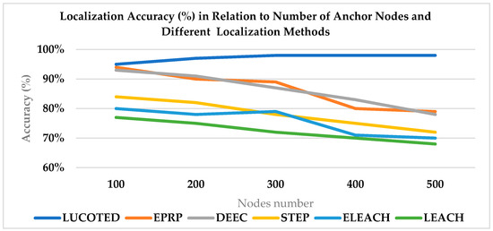
Figure 2. Comparison of various localization techniques accuracy based on the number of nodes over 100.

The graph below, Figure 3 shows that in the same randomly generated environment of simulation, our method LUCOTED, gives a better accuracy as average values, reaching 97.7%, while the gradient descent method realizes 78.19%. Far from this value, the trilateration approach does not surpass 70% because of its dependency on the initial position of the unknown node and anchor nodes. In fact, this technique, from time to time, produces results that violate the simulation’s constraints.

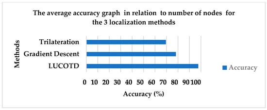
Figure 3. The average accuracy graph in relation to number of nodes for the 3 localization methods.

The tableau below Table 2 displays the average values of unknown node coordinates, precision of location, energy required and iteration for each of the three approaches as provided by experimental simulation.

Table 2. Data, generated by the experimentation, expressed in mean values for each method.

Average Value	X	Y	Z	Accuracy	Energy (104j)	Iterations
LUCOTD	64.07	49.34	38.45	97.70	796.15	600
Gradient Descent	45.81	43.52	43.10	78.19	2361.94	600
Trilateration	54.98	49.78	52.33	69.44	1.39

In Figure 4, our localization technique, LUCOTED, provides a higher level of accuracy than the trilateration-based localization method, which is used as a reference in research [36], because of its respected accuracy by considering the same simulation variables (45 s, 100 nodes, x, y, −z = 1000).

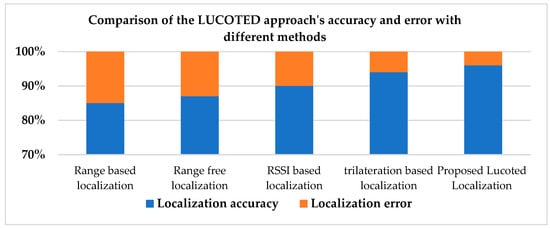
Figure 4. Accuracy and error between LUCOTED and other techniques.

In the next graph (Figure 5), in which we adopt Trilateration method as baseline for normalization of energy, we observe that the LUCOTED approach consumes less energy than Gradient Descent but more than Trilateration method. This result is appreciable and highly significant because the first two methods are iterative, the Trilateration is direct and uses a lower energy consumption. In fact, in this case, there will be a trade-off to be made between the necessary energy and location accuracy.

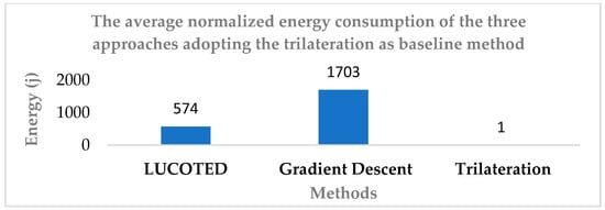
Figure 5. Comparison of normalized energy consumption between LUCOTED, Gradient Descent, and Trilateration methods.

In Figure 6 below, the proposed LUCOTED in blue, has the lowest error as compared to other localization methods. Its value actually drops from 9.8 to 3.2 as the number of nodes increases from 20 to 80. Our method is more successful than the localization approach DGGDEA that employs the DEEC Gaussian Gradient Distance algorithm, as well as other techniques of localization related to the same study referenced in [36].

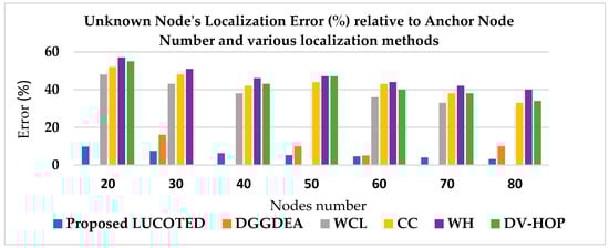
Figure 6. Comparing the error of localization techniques according the number of nodes between 20 and 80.

6. Conclusions

In addition to its impact on human activities in aquatic areas, the relevance of our localization technique compared to other approaches can be specified as follows:

• Primarily through simulation:
  • It offers better location accuracy compared to trilateration and gradient descent methods and to other recent approaches.
  • It consumes less energy than gradient descent as an iterative method.
  • It provides solutions that respect constraints related to the communication range and boundary of the simulation’s area.
  • It guarantees always convergence.
• Secondly, through the algorithmic aspect:
  • LUCOTED outperforms other methods because it allows the solving of a localization problem with constraints independently of the simulation’s initial condition.
• The UWSN makes it possible to prevent the risk of human losses by monitoring watery environments.

References

- FAO. The State of World Fisheries and Aquaculture; Blue Transformation in Action: Rome, Italy, 2024. [Google Scholar]
- Jahanbakht, M.; Xiang, W.; Hanzo, L.; Azghadi, M.R. Internet of Underwater Things and Big Marine Data Analytics—A Comprehensive Survey. IEEE Commun. Surv. Tutorials 2021, 23, 904–956. [Google Scholar] [CrossRef]
- Yang, G.; Dai, L.; Wei, Z. Challenges. Threats, Security Issues and New Trends of Underwater Wireless Sensor Networks. Sensors 2018, 18, 3907. [Google Scholar] [CrossRef] [PubMed]
- Oliveira, H.A.; Nakamura, E.; Loureiro, A.; Boukerche, A. Directed Position Estimation: A Recursive Localization Approach for Wireless Sensor Networks. In Proceedings of the 14th International Conference on Computer Communications and Networks, San Diego, CA, USA, 17–19 October 2005; pp. 557–562. [Google Scholar] [CrossRef]
- Xu, Z.; He, D.; Li, J.; Jiang, L.; Wang, H. Correction method for TOA measurement of target signal based on Kalman Filter. In Proceedings of the 2017 IEEE 2nd Advanced Information Technology, Electronic and Automation Control Conference (IAEAC), Chongqing, China, 25–26 March 2017; pp. 230–235. [Google Scholar] [CrossRef]
- Cao, H.; Chan, Y.T.; So, H.C. Compressive TDOA Estimation: Cramér-Rao Bound and Incoherent Processing. IEEE Trans. Aerosp. Electron. Syst. 2020, 56, 3326–3331. [Google Scholar] [CrossRef]
- Arenas, M.; Podhorski, A.; Arrizabalaga, S.; Goya, J.; Sedano, B.; Mendizabal, J. Implementation and validation of an Angle of Arrival (AOA) determination system. In Proceedings of the 2015 Conference on Design of Circuits and Integrated Systems (DCIS), Estoril, Portugal, 25–27 November 2015; pp. 1–7. [Google Scholar] [CrossRef]
- Xe, W.; Li, Q.; Hua, X.; Yu, K.; Qiu, W.; Zhou, B. A New Algorithm for Indoor RSSI Radio Map Reconstruction. IEEE Access 2018, 6, 76118–76125. [Google Scholar] [CrossRef]
- Luo, Q.; Yang, K.; Yan, X.; Li, J.; Wang, C.; Zhou, Z. An Improved Trilateration Positioning Algorithm with Anchor Node Combination and K-Means Clustering. Sensors 2022, 22, 6085. [Google Scholar] [CrossRef]
- Rajagopal, A.; Somasundaram, S.; Sowmya, B.; Suguna, T. Soft computing-based cluster head selection in wireless sensor network using bacterial foraging optimization algorithm. Int. J. Electron. Commun. Eng. 2015, 3, 379–384. [Google Scholar] [CrossRef]
- Beniwal, M.; Singh, R. Localization techniques and their challenges in underwater wireless sensor networks. Int. J. Comput. Sci. Inf. Technol. 2014, 5, 4706–4710. [Google Scholar]
- Niculescu, D.; Nath, B. Ad Hoc Positioning System (APS). In Proceedings of the IEEE GLOBECOM ’01, San Antonio, TX, USA, 25–29 November 2001; pp. 2926–2931. [Google Scholar] [CrossRef]
- Boukerche, A.; Oliveira, H.A.B.; Nakamura, E.F.; Loureiro, A.A.F. Secure localization algorithms for wireless sensor networks. IEEE Commun. Mag. 2008, 46, 96–101. [Google Scholar] [CrossRef]
- Nain, M.; Goyal, N.; Dhurandher, S.K.; Dave, M.; Verma, A.K.; Malik, A. A survey on node localization technologies in UWSNs: Potential solutions, recent advancements, and future directions. Int. J. Commun. Syst. 2024, 37, e5915. [Google Scholar] [CrossRef]
- Pu, W.Y. A Survey of Localization Techniques for Underwater Wireless Sensor Networks. J. Comput. Electron. Inf. Manag. 2023, 11, 10–15. [Google Scholar] [CrossRef]
- Jouhari, M.; Ibrahimi, K.; Tembine, H.; Ben-Othman, J. Underwater wireless sensor networks: A survey on enabling technologies, localization protocols, and internet of underwater things. IEEE Access 2019, 7, 96879–96899. [Google Scholar] [CrossRef]
- Jim, P.; Kurose, J.; Levine, B.N. A survey of practical issues in underwater networks. ACM SIGMOBILE Mob. Comput. Commun. Rev. 2007, 11, 23–33. [Google Scholar] [CrossRef]
- Heidemann, J.; Ye, W.; Wills, J.; Syed, A.; Li, Y. Research challenges and applications for underwater sensor networking. In Proceedings of the IEEE Wireless Communications and Networking Conference, WCNC2006, Las Vegas, NV, USA, 3–6 April 2006; Volume 1, pp. 228–235. [Google Scholar] [CrossRef]
- Alkan, R.M.; Kalkan, Y.; Aykut, N.O. Sound velocity determination with empirical formulas and bar check. In Proceedings of the 23rd FIG Congress, Munich, Germany, 8–13 October 2006; pp. 1–14. [Google Scholar]
- Ouidir, H.; Berqia, A.; Aouad, S. Improving UWSN Performance using Reinforcement Learning Algorithm QENDIP. In Proceedings of the 2024 11th International Conference on Wireless Networks and Mobile Communications (WINCOM), Leeds, UK, 23–25 July 2024. [Google Scholar] [CrossRef]
- Li, H.; He, Y.; Cheng, X.; Zhu, H.; Sun, L. Security and privacy in localization for underwater sensor networks. IEEE Commun. Mag. 2015, 53, 56–62. [Google Scholar] [CrossRef]
- Nanthakumar, S.; Jothilakshmi, P. A comparative study of range based and range free algorithms for node localization in underwater. E-Prime—Adv. Electr. Eng. Electron. Energy 2024, 9, 100727. [Google Scholar] [CrossRef]
- Agarwal, A.K.; Khan, G.; Qamar, S.; Lal, N. Localization and correction of location information for nodes in UWSN-LCLI. Adv. Eng. Softw. 2022, 173, 103265. [Google Scholar] [CrossRef]
- Han, G.; Jiang, J.; Shu, L.; Xu, Y.; Wang, F. Localization Algorithms of Underwater Wireless Sensor. Sensors 2012, 12, 2026–2061. [Google Scholar] [CrossRef]
- Rani, S.; Anju; Sangwan, A.; Kumar, K.; Nisar, K.; Soomro, T.R.; Ibrahim, A.A.A.; Gupta, M.; Chand, L.; Khan, S.A. Review and Analysis of Localization Techniques in Underwater Wireless Sensor Networks. Computer. Mater. Contin. 2023, 75, 5697–5715. [Google Scholar] [CrossRef]
- Xu, T.; Hu, Y.; Zhang, B.; Leus, G. RSS-based sensor localization in underwater acoustic sensor networks. In Proceedings of the IEEE International Conference on Acoustics, Speech and Signal Processing (ICASSP), Shanghai, China, 20–25 March 2016. [Google Scholar] [CrossRef]
- Yang, B.; Guo, L.Y.; Guo, R.J.; Zhao, M.M.; Zhao, T.T. A Novel Trilateration Algorithm for RSSI-Based Indoor Localization. IEEE Sens. J. 2020, 20, 8164–8172. [Google Scholar] [CrossRef]
- Yan, X.; Luo, Q.; Yang, Y.; Liu, S.; Li, H.; Hu, C. ITL-MEPOSA: Improved Trilateration Localization with Minimum Uncertainty Propagation and Optimized Selection of Anchor Nodes for Wireless Sensor Networks. IEEE Access 2019, 7, 53136–53146. [Google Scholar] [CrossRef]
- Zhou, Z.; Zhou, X.; Xing, G.; Jin, Z.; Chen, Y.; Yang, Q. Localization of Underwater Wireless Sensor Networks for Ranging Interference based on the AdaDelta Gadient Descent Algorithm. Wireless. Pers. Commun. 2024, 137, 1189–1216. [Google Scholar] [CrossRef]
- Wang, P.; Wang, X.; Li, W.; Fan, X.; Zhao, D. DV-Hop localization based on Distance Estimation using Multi-node and Hop Loss in IoT. TechRxiv 2024. [Google Scholar] [CrossRef]
- Martin, R.; Zhu, Y.; Pu, L.; Dou, F.; Peng, Z.; Cui, J.-H.; Rajasekaran, S. Aqua-Sim Next Generation: A NS-3 Based Simulator for UWSN. In Proceedings of the 10th International Conference on Underwater Networks & Systems, Arlington, VA, USA, 22–24 October 2015. [Google Scholar] [CrossRef]
- Namesh, C.; Ramakrishnan, B. Analysis of VBF protocol in underwater sensor network for static and moving nodes. Int. J. Computer. Netw. Appl. 2015, 2, 20–26. [Google Scholar]
- Shenbagharaman, A.; Paramasivan, B. Trilateration method-based node localization and energy efficient routing using rsa for under water wireless sensor network. Sustain. Comput. Inform. Syst. 2024, 41, 100952. [Google Scholar] [CrossRef]
- Sehgal, A.; David, C.; Schonwalder, J. Energy Consumption in Underwater Acoustic Sensor Networks. In Proceedings of the OCEANS’11 MTS/IEEE KONA, Waikoloa, HI, USA, 19–22 September 2011. [Google Scholar] [CrossRef]
- Bennouri, H.; Berqia, A.; Patrick, N.K. U-NewReno transmission control protocol to improve TCP performance in UWSN. J. King Saud Univ.-Comput. Inf. Sci. 2022, 34, 5746–5758. [Google Scholar] [CrossRef]
- Aroba, O.J.; Naicker, N.; Adeliyi, T.T. Node localization in wireless sensor networks using a hyper-heuristic DEEC-Gaussian gradient distance algorithm. Sci. Afr. 2023, 19, e01560. [Google Scholar] [CrossRef]
Disclaimer/Publisher’s Note: The statements, opinions and data contained in all publications are solely those of the individual author(s) and contributor(s) and not of MDPI and/or the editor(s). MDPI and/or the editor(s) disclaim responsibility for any injury to people or property resulting from any ideas, methods, instructions or products referred to in the content. |
© 2025 by the authors. Licensee MDPI, Basel, Switzerland. This article is an open access article distributed under the terms and conditions of the Creative Commons Attribution (CC BY) license (https://creativecommons.org/licenses/by/4.0/).