Abstract
Accurate tumor segmentation is crucial for cancer diagnosis and treatment planning. We developed a hybrid framework combining complementary convolutional neural network (CNN) models and advanced post-processing techniques for robust segmentation. Model 1 uses contrast-limited adaptive histogram equalization preprocessing, CNN predictions, and active contour refinement, but struggles with complex tumor boundaries. Model 2 applies noise-augmented preprocessing and iterative detection to enhance the segmentation of subtle and irregular regions. The outputs of both models are merged and refined with edge correction, size filtering, and a spatial intensity metric (SIM) expansion to improve under-segmented areas, an approach that achieves higher F1 scores and intersection over union scores. The developed framework highlights the potential in combining machine learning and image-processing techniques to develop reliable diagnostic tools.
1. Introduction
Tumor detection plays a pivotal role in medical image analysis, enabling early diagnosis and effective treatment of cancer [1,2,3,4,5,6,7,8,9,10]. Automated tumor segmentation algorithms have emerged as valuable tools for medical professionals, showing the potential to accurately and efficiently identify tumor regions [1,2,3,4,5,6,7,8]. These algorithms reduce the burden of manual segmentation, while improving diagnostic consistency and precision.
Despite significant advancements, the development of robust tumor detection methods remains challenging due to the high variability in tumor characteristics across different imaging modalities and cancer types. Variations in the shape, size, texture, and intensity of tumors, combined with differences in imaging technologies such as magnetic resonance imaging (MRI) [6,7,11,12], computed tomography (CT), and ultrasound, necessitate sophisticated techniques to achieve reliable performance.
In this study, we developed and evaluated a novel approach to tumor detection using convolutional neural networks (CNNs). We designed and implemented the CNN architecture, as well as the evaluation metrics used to measure the effectiveness of the proposed method. A series of experiments were conducted under varying conditions, with the results providing insights into the performance of the model and highlighting areas for improvement. The limitations of the current approach and potential directions for future development were then determined, aiming to further enhance the accuracy and robustness of tumor detection algorithms.
2. Materials and Methods
A tumor detection algorithm was developed in the following process.
2.1. Morphological Processing
In morphological processing, we used a structuring element, a small binary matrix, to define the neighborhood for processing. In erosion, objects shrink by removing boundary pixels, eliminating noise, and separating connected objects. A pixel is retained only if all pixels under the structuring element are in the foreground. In dilation, objects are expanded by adding boundary pixels in order to bridge gaps, enhance connectivity, and fill holes. A pixel is added if any pixel under the structuring element is in the foreground.
2.2. Gaussian Filter
The Gaussian filter is a widely used image-processing technique used for smoothing and noise reduction. A Gaussian function is applied to the image, effectively averaging pixel intensities and preserving edges rather than simple averaging filters. The filter is named after the Gaussian distribution, which is characterized by its bell-shaped curve (Equation (1)).
where x and y are spatial coordinates and σ is the standard deviation, controlling the filter’s spread and smoothing strength.
2.3. CLAHE
CLAHE is an advanced image-processing technique that enhances contrast while minimizing noise amplification. Unlike standard histogram equalization, CLAHE operates locally, dividing the image into small tiles and redistributing pixel intensities based on local histograms. To prevent excessive noise in uniform areas, it clips the histogram at a threshold and redistributes the clipped values. This adaptive method preserves details in both bright and dark regions. CLAHE combines the processed tiles smoothly using bilinear interpolation to avoid boundary artifacts. It is particularly effective for medical images, low-light photos, and applications needing local contrast enhancement.
2.4. Active Contour Model
The active contour model, or Snake model, is a technique for image segmentation and object boundary detection. It represents a deformable curve that adjusts to fit object contours by minimizing an energy function influenced by three forces: internal forces for smoothness, image forces derived from intensity gradients used to guide the curve to the edges, and external constraint forces used to focus on specific regions. By balancing these forces, the model effectively detects boundaries while maintaining curve continuity.
2.5. IoU
IoU is used to evaluate the accuracy of object detection and segmentation by measuring the overlap between the predicted region and the ground truth region , as described in the following. IoU ranges from 0 to 1, where 1 indicates perfect overlap, and 0 indicates no overlap. Higher IoU values signify better alignment with the ground truth (Equation (2)).
- : Overlap area between predicted and ground truth regions;
- : Total area covered by both regions.
2.6. F1 Score
The F1 score is a performance metric utilized for classification tasks, particularly in imbalanced datasets. It is the harmonic mean of precision and recall (Equation (3)). The F1 score ranges from 0 to 1, with higher values indicating better performance. It balances precision and recall, making it useful in cases where false positives and false negatives carry significant costs or class distributions are imbalanced.
Precision is the proportion of correctly identified positive predictions out of all positive predictions.
Recall is the proportion of correctly identified positive predictions out of all actual positive cases.
2.7. Spatial Intensity Metric (SIM)
Segmentation refinement is conducted using SIM, which combines spatial and intensity-based constraints. Contours are extracted from the binary mask, and up to 8 evenly spaced key points along the boundary are selected. For each key point , a search area is defined, and each pixel is evaluated based on its spatial distance from the key point. The intensity difference is determined relative to the reference intensity. The SIM is calculated as follows. Pixels with SIM below a threshold are added to the expanded mask. Expanded regions are merged with the original mask, and the largest connected region is selected. Internal holes are filled to produce a refined, contiguous segmentation mask.
2.8. Region Exclusion Based on Geometric Features
Unwanted regions are excluded based on shape and size in the binary mask. If fewer than two components exist, the mask remains unchanged. For multiple regions, contours are extracted, and the largest contour is selected. Then, the points where the contour has a large curvature are selected, as in Figure 1. Contours with fewer than five points are skipped, and an ellipse is fitted to the largest contour using the least-squares method, providing the following key parameters.
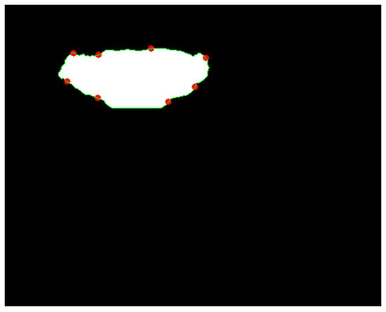
Figure 1.
An example of selected points. The green curve is the contour and the red points are the selected points.
- Center: ;
- Semi-major axis: , Semi-minor axis: ;
- Rotation angle: .
A pixel lies within the ellipse if it satisfies the ellipse equation. The major and minor axes are compared, and regions with an axis ratio exceeding a certain threshold (too elongated) are excluded. The intersection area between the region and the ellipse mask is then calculated. Regions with an overlap ratio above the threshold are retained; otherwise, they are excluded as artifacts. This process ensures that only regions with balanced proportions and sufficient overlap are included in the final mask. An example that applies an ellipse to approximate a segmented region is shown in Figure 2.
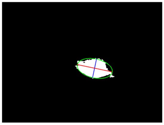
Figure 2.
An example of a geometric feature. The red line is the long axis, the blue line is the short axis, and the green curve is the border of the ellipse.
After processing all regions, the valid regions are combined into a unified binary mask. If no valid regions remain, the original mask is returned to preserve input integrity. This method ensures that the retained regions exhibit consistent geometric features, such as ellipticity.
3. Results
3.1. Initialization
First, Models 1 and 2 preprocess medical images to prepare them for tumor detection, with slight differences in their approaches. Model 1 emphasizes noise reduction and contrast enhancement, using Gaussian Blur (5 × 5 kernel, sigma 1.5), brightness adjustment to a target value of 120, and CLAHE (clip limit 4.0, tile grid size 8 × 8) to enhance local contrast and reveal finer details.
Model 2 focuses on robustness by adding Gaussian noise (a mean of 0 and a standard deviation (SD) of 30) to simulate variability. It also applies brightness adjustment to a target of 120 and Gaussian Blur (5 × 5 kernel, sigma 1.5) for noise reduction, but omits CLAHE, retaining the original contrast of the images. Both models have grid divisions with 16 × 16 pixel grids, and label each grid as “Tumor” or “Normal Tissue”, based on the percentage of tumor pixels, for localized analysis. The detailed layer structure of the model is shown in Table 1.

Table 1.
Layer structure.
In this study, the performance of the two preprocessing methods was evaluated based on their ability to predict whether each grid corresponds to a tumor or normal tissue, with the test accuracy determined as follows. The test accuracies using Models 1 and 2 are shown in Table 2.
Table 2.
CNN models’ test accuracy.
3.2. First Experiment: Tumor Segmentation by Model 1
The following was the flow of tumor detection using Model 1.
- Tumor prediction using CNN Model 1: Grayscale medical images are preprocessed with CLAHE for contrast enhancement and Gaussian Blur for noise reduction. The images are divided into 16 × 16 pixel grids and classified using a pre-trained CNN model. Tumor regions (confidence > 0.3) are marked in a tumor mask, with adjacent grids connected to ensure spatial continuity.
- Active contour refinement: The Chan–Vese Active Contour Model is used to refine tumor boundaries, using the tumor mask as the initial contour. Contours evolve to align with true boundaries, retaining only regions with significant overlap with the CNN-predicted mask.
- Size filtering: Small regions (<0.1% of the image area) are removed as noise, and large regions (>17%) are split into smaller components, using morphological operations.
- Ellipse fitting: An ellipse is fitted to each segmented region, retaining regions with significant overlap (≥60%) between the ellipse and the original contour.
- Hole filling: Internal holes in tumor regions are filled to ensure continuous masks.
- Edge removal: Small regions touching image edges are excluded, focusing on central tumor areas in the final output.
The experimental results for tumor segmentation using Model 1 were evaluated using F1 score and IoU. The detailed results and their distribution are presented in Table 3 and Figure 3. F1 and IoU scores showed significant variability, with most predictions indicating low overlap and precision, though several cases presented reasonable accuracy. Tumor detection accuracy heavily depended on the CNN’s initial predictions, which significantly influenced overall performance. However, Model 1 showed lower accuracy, negatively impacting the final segmentation results.
Table 3.
Average F1 and IoU scores using Model 1.
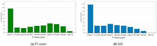
Figure 3.
F1 and IoU scores for Model 1.
3.3. Second Experiment: Using Model 2
While Model 1 employs CLAHE preprocessing and a CNN-based initial prediction, Model 2 introduces noise-addition techniques and iterative refinement to complement Model 1’s predictions.
- Tumor prediction using CNN Model 2: Model 2 preprocesses input grayscale images by adding Gaussian noise (μ = 0, σ = 30) to simulate real-world variations, followed by Gaussian filtering for noise reduction. Unlike Model 1, it retains the original contrast, focusing on inherent image features. Grids with a confidence score > 0.3 are classified as tumor regions.
- Iterative detection: Using the Chan–Vese Active Contour Model, Model 2 refines tumor boundaries over five iterations. Each iteration includes size filtering, ellipse fitting, hole filling, and edge removal. The resulting masks are combined into a cumulative confidence mask, with a 60% confidence threshold applied to generate the final tumor prediction results.
The performance of Model 2 was evaluated independently. The average F1 and IoU scores were 0.2343 and 0.1870, both significantly lower than the scores of Model 1. The F1 and IoU score distributions (Figure 4) were within the range of 0.0–0.1, highlighting the limited segmentation accuracy of the model. Model 2’s lower levels of performance stem from the absence of contrast enhancement during preprocessing. Unlike Model 1, which uses CLAHE to improve visibility, Model 2 relies on original contrast, struggling with low-contrast or irregular tumor regions (Table 4 and Figure 4).
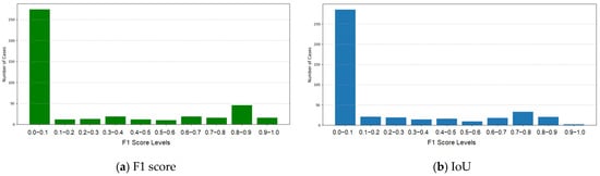
Figure 4.
F1 and IoU scores for Model 2.
Table 4.
Average F1 and IoU scores for Model 2.
3.4. Third Experiment: Using Merged Model
Tumor masks from Models 1 and 2 were merged using a logical OR operation to include all detected tumor regions. Morphological operations, such as erosion and dilation, were applied to reduce false positives near the edges, and size filtering was used to ensure accurate segmentation. By combining both models, their complementary strengths were utilized for a more robust tumor detection. The experimental results of tumor segmentation merging Models 1 and 2 were evaluated using F1 and IoU scores. The detailed results and their distributions are presented in Table 5 and Figure 5. The combined model achieved an average F1 score of 0.4714, demonstrating an improvement in the balance between precision and recall, compared with Model 1. The average IoU score was 0.3874, reflecting better overlap and alignment between the predicted tumor regions and the ground truth. While the majority of cases were concentrated in the range of 0.0–0.1, there was a noticeable increase in cases achieving higher IoU scores (e.g., 0.6–0.7, 0.7–0.8, and 0.8–0.9), reflecting the more accurate tumor boundary segmentation in these instances.
Table 5.
Average F1 and IoU scores using the merged model.
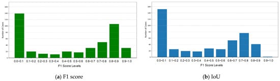
Figure 5.
F1 and IoU scores for the merged model.
3.5. Fourth Experiment: Using Refined Merged Model
To address under-segmentation in the merged mask, SIM expansion was used to refine tumor boundaries by adding pixels based on spatial and intensity-based thresholds. The expanded mask was combined with the original mask using a logical OR operation, retaining the largest connected region. Holes are filled for continuity, resulting in a more complete and refined segmentation. The refined merged model, incorporating SIM expansion, demonstrated significant improvements in segmentation accuracy. The enhanced model achieved an average F1 score of 0.5450, indicating an improved balance between precision and recall, compared to the previous merged model. The average IoU score increased to 0.4460, reflecting a more precise overlap between the predicted tumor regions and the ground truth. The distribution showed a remarkable improvement in high-performing cases. Substantial increases were observed in the cases where the F1 score in the ranges of 0.8–0.9 and 0.9–1.0. Although the proportion of cases in the lowest range (0.0–0.1) decreased, low-scoring cases remained, indicating challenges in handling certain tumor patterns (Table 6 and Figure 6).
Table 6.
Average F1 and IoU scores using the refined merged Model1.
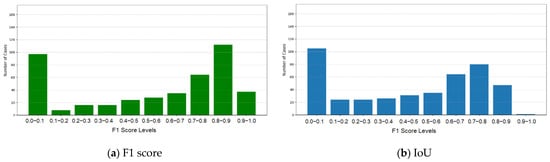
Figure 6.
F1 and IoU scores for the refined merged model.
4. Discussion and Conclusions
We developed a progressive tumor segmentation approach for medical imaging by integrating multiple models and refining methodologies for improved accuracy. Model 1, with robust preprocessing and active contour refinement, enabled initial tumor predictions but struggled with complex boundaries and intensity variations, resulting in lower F1 and IoU scores. To address these issues, Model 2 was constructed, utilizing noise-augmented preprocessing and iterative refinement, enhancing consistency and accuracy. However, challenges with under-segmentation and boundary inconsistencies persisted, particularly for low-contrast or irregular tumor shapes. An enhanced merged model was developed using SIM expansion to refine boundaries and expand tumor regions based on spatial and intensity-based relationships. This significantly improved segmentation accuracy, addressing under-segmentation and incomplete delineation. Overall, the hybrid framework combining complementary models, iterative refinement, and advanced post-processing techniques demonstrated superior performance but highlighted the need for further improvements in handling low-contrast, irregular tumor regions.
For further improvement, the current grid-based method segments images into 16 × 16 pixel grids, classifying each as tumor or normal tissue. While effective, this approach struggles with large tumors, leading to under-segmentation or boundary inaccuracies. Increasing grid resolution or using adaptive grid sizes based on tumor characteristics addresses this limitation. For future enhancement, the incorporation of local texture analysis could be used to distinguish malignant tumors from benign tumors. High-resolution grids paired with advanced feature extraction enable simultaneous tumor segmentation and malignancy assessment, offering more comprehensive diagnostic insights.
Author Contributions
Conceptualization, D.O. and J.-J.D.; methodology, D.O. and J.-J.D.; software, D.O.; validation, D.O.; formal analysis, D.O. and J.-J.D.; investigation, D.O.; resources, D.O.; data curation, D.O.; writing—original draft, D.O.; writing—review and editing, D.O. and J.-J.D.; visualization, D.O.; supervision, J.-J.D.; project administration, J.-J.D.; funding acquisition, J.-J.D. All authors have read and agreed to the published version of the manuscript.
Funding
This research was funded by the National Science and Technology Council, Taiwan, under the contract of NSTC 113-2221-E-002-146.
Institutional Review Board Statement
Not applicable.
Informed Consent Statement
Not applicable.
Data Availability Statement
The original contributions presented in the study are included in the article, further inquiries can be directed to the authors.
Conflicts of Interest
The authors declare no conflicts of interest.
References
- Kaus, M.R.; Warfield, S.K.; Nabavi, A.; Black, P.M.; Jolesz, F.A.; Kikinis, R. Automated Segmentation of MR Images of Brain Tumors. Radiology 2001, 218, 586–591. [Google Scholar] [CrossRef] [PubMed]
- Prastawa, M.; Bullitt, E.; Ho, S.; Gerig, G. A brain tumor segmentation framework based on outlier detection. Med. Image Anal. 2004, 8, 275–283. [Google Scholar] [CrossRef] [PubMed]
- Nanda, A.; Barik, R.C.; Bakshi, S. SSO-RBNN driven brain tumor classification with Saliency-K-means segmentation technique. Biomed. Signal Process. Control 2023, 81, 104356. [Google Scholar] [CrossRef]
- Usman Akbar, M.; Larsson, M.; Blystad, I.; Eklund, A. Brain tumor segmentation using synthetic MR images—A comparison of GANs and diffusion models. Sci. Data 2024, 11, 259. [Google Scholar] [CrossRef] [PubMed]
- Wang, T.; Cheng, I.; Basu, A. Fluid vector flow and applications in brain tumor segmentation. IEEE Trans. Biomed. Eng. 2009, 56, 781–789. [Google Scholar] [CrossRef] [PubMed]
- Khotanlou, H.; Colliot, O.; Atif, J.; Bloch, I. 3D brain tumor segmentation in MRI using fuzzy classification, symmetry analysis and spatially constrained deformable models. Fuzzy Sets Syst. 2009, 160, 1457–1473. [Google Scholar] [CrossRef]
- Kermi, A.; Andjouh, K.; Zidane, F. Fully automated brain tumour segmentation system in 3D-MRI using symmetry analysis of brain and level sets. IET Image Process. 2018, 12, 1964–1971. [Google Scholar] [CrossRef]
- Khosravanian, A.; Rahmanimanesh, M.; Keshavarzi, P.; Mozaffari, S.; Kazemi, K. Level set method for automated 3D brain tumor segmentation using symmetry analysis and kernel induced fuzzy clustering. Multimed. Tools Appl. 2022, 81, 21719–21740. [Google Scholar] [CrossRef]
- Abd-Ellah, M.K.; Awad, A.I.; Khalaf, A.A.M.; Hamed, H.F.A. Design and implementation of a computer-aided diagnosis system for brain tumor classification. In Proceedings of the International Conference on Microelectronics, Giza, Egypt, 17–20 December 2016; pp. 73–76. [Google Scholar]
- Rasool, M.; Ismail, N.A.; Boulila, W.; Ammar, A.; Samma, H.; Yafooz, W.M.; Emara, A.H.M. A hybrid deep learning model for brain tumor classification. Entropy 2022, 24, 799. [Google Scholar] [CrossRef] [PubMed]
- Zhang, Y.; Dong, Z.; Wu, L.; Wang, S. A hybrid method for MRI brain image classification. Expert. Syst. Appl. 2011, 38, 10049–10053. [Google Scholar] [CrossRef]
- El-Dahshan, E.S.A.; Hosny, T.; Salem, A.B.M. Hybrid intelligent techniques for MRI brain images classification. Digit. Signal Process. 2010, 20, 433–441. [Google Scholar] [CrossRef]


Disclaimer/Publisher’s Note: The statements, opinions and data contained in all publications are solely those of the individual author(s) and contributor(s) and not of MDPI and/or the editor(s). MDPI and/or the editor(s) disclaim responsibility for any injury to people or property resulting from any ideas, methods, instructions or products referred to in the content. |
© 2025 by the authors. Licensee MDPI, Basel, Switzerland. This article is an open access article distributed under the terms and conditions of the Creative Commons Attribution (CC BY) license (https://creativecommons.org/licenses/by/4.0/).