Application of Machine Learning for Optimizing Chemical Vapor Deposition Quality ^†

Abstract

Chemical vapor deposition (CVD) is a high-precision thin-film fabrication technique that is widely applied in semiconductor manufacturing, optical component manufacturing, and materials science. The performance of the deposition process plays a critical role in determining the quality of the final product. However, multiple variables in CVD processes have a highly nonlinear nature that involves complex interactions. Therefore, conventional experimental methods exhibit limitations in quality control and process optimization for CVD. In this study, we developed a predictive model based on process parameters and quality indicators using machine learning techniques to analyze and optimize the CVD processes. Through data collection, feature selection, model training, and model validation, the developed machine-learning algorithms were tested and evaluated. The adopted machine learning algorithms effectively captured the nonlinear relationships between multiple variables in CVD processes, accurately predicted thin-film quality indicators, and provided data for optimizing process parameters. In addition, the analysis results of feature importance revealed the effect of each key parameter on product quality, offering a basis for process improvement. Overall, the results of this study highlight the capability of machine learning algorithms for quality control and optimization in CVD processes for future advancements in smart manufacturing.

1. Introduction

Chemical vapor deposition (CVD) is a thin-film deposition technique that is widely used in the manufacturing of semiconductor products, optical components, solar cells, and various high-performance materials. CVD involves introducing volatile gaseous precursors into a reaction chamber, in which a substrate is heated to an adequate temperature. The precursor undergoes decomposition or chemical reactions on the substrate surface to form solid-phase products that lead to the creation of a uniform thin film. The gaseous by-products generated during the reaction are removed from the chamber through an exhaust system.

Common gaseous precursors include argon, nitrogen, and hydrogen sulfide. The heating temperature of the chamber typically ranges from 200 to 1050 °C, depending on the materials being processed. Pressure control is necessary under atmospheric and low-pressure conditions, with the corresponding processes called atmospheric-pressure CVD and low-pressure CVD. The reaction chamber is a sealed deposition chamber designed for gas supply and reaction (Figure 1).

The key process parameters affecting thin-film quality are chamber pressure, the flow rates of the precursor and reactive gas, the vacuum exhaust flow rate, substrate temperature, ambient temperature, and the flow rate and temperature of cooling water. First, the chamber pressure during deposition influences the precursor flow rate, reactive gas flow rate, and exhaust speed. Second, the flow rates of the precursor and reactive gas affect the optimal elemental composition of the material, and achieving an ideal composition ratio in practical processes is challenging. Third, the vacuum exhaust flow rate is determined by the extent to which the main valve opens; a high gas flow rate leads to a low deposition rate, which causes varying effects on thin-film quality. Fourth, substrate temperature affects film uniformity, the required reaction temperature for compound formation, and substrate–material compatibility as one of the most critical process parameters in CVD systems. Fifth, ambient temperature has a notable effect on specific vacuum pumps; large temperature fluctuations can reduce vacuum efficiency considerably. Finally, the flow rate and temperature of cooling water are key parameters in CVD. Cooling water is primarily used during standby and deposition to prevent the CVD equipment from overheating, which leads to thermal degradation, O-ring aging, and cracks that hinder vacuum sealing. The interactions among the six process parameters markedly affect the thickness, uniformity, structure, and performance of the deposited thin films.

Conventional quality control methods are mainly based on physical models or experimental trials. However, these methods exhibit limitations when they are applied to highly nonlinear systems with multiple variables. With the accumulation of process data, data-driven analytical methods are required to explore CVD processes. With its advantages in pattern recognition and predictive modeling, machine learning offers new opportunities for optimizing CVD quality. In this study, we developed an accurate model based on process data to predict thin-film quality, leveraging machine learning algorithms.

2. Methods

The methodology of this study consisted of the following steps (Figure 2): data collection, data preprocessing, feature selection, model construction, experimental validation and optimization, and result comparison. First, historical and real-time monitoring data of CVD, including temperature, pressure, gas flow rates, and thin-film quality measurements, were collected. Second, the collected data were subjected to cleaning, standardization, and feature extraction to remove noise and extract key features. Third, feature selection was performed using methods such as analysis of variance (ANOVA), the least absolute shrinkage and selection operator (LASSO) [1], principal component analysis (PCA), and mutual information analyses to identify the most relevant features, thereby enhancing model performance, reducing overfitting, and improving interpretability. Fourth, four machine learning algorithms, namely linear regression [1], extreme gradient boosting (XGBoost) [1,2,3,4], random forest [1,3], and support vector regression (SVR) [2,5], were employed to construct models for predicting thin-film quality. The performance of these models was compared, and their hyperparameters were optimized through cross-validation and grid search to increase their predictive accuracy (Figure 3). Fifth, the CVD process was adjusted on the basis of the results obtained with the four developed machine learning models, and the effectiveness of the adjusted process in real-world production was evaluated. Finally, the performance of the four machine learning models was assessed in different scenarios for CVD thin-film deposition, which enabled the identification of the most appropriate model.

2.1. Data Collection

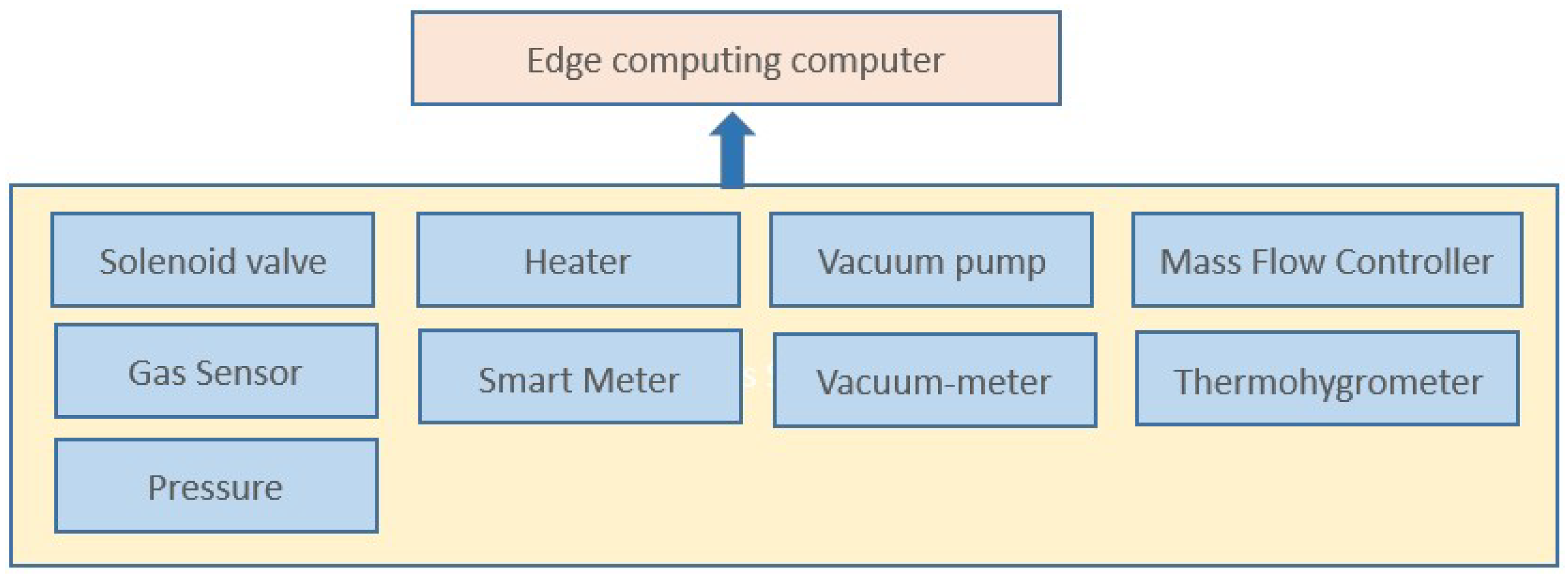
Sensor and power consumption data were obtained from a CVD system (Figure 4).

2.2. Data Preprocessing

Data preprocessing is a critical step because data quality directly affects model performance. Data preprocessing is conducted to transform raw data into a format suitable for machine learning models, thus ensuring more accurate learning and prediction. In this study, datasets from various sources were integrated, and columns with excessive missing values and duplicate data were removed. Then, standardization and normalization were conducted. The data were split into training, validation, and test sets to evaluate model performance. Random sampling and cross-validation techniques were applied to enhance model stability. The adequate data processing improved model performance and mitigated problems such as overfitting and underfitting, thereby leading to more precise predictions.

2.3. Feature Selection

Multiple techniques were employed to identify key features. Specifically, ANOVA was used to determine the presence of significant differences in means across multiple data groups. In LASSO regression, L1 regularization was adopted to reduce several feature coefficients to 0. In addition, PCA was performed to project high-dimensional data onto a lower-dimensional space to extract principal features. Features were extracted by identifying the directions of maximum variance in the dataset. Finally, mutual information analyses were conducted to quantify the dependence between two random variables and assess the correlations between features and the target variable.

2.4. Model Construction, Validation, and Optimization

Four machine learning algorithms, namely logistic regression, support vector regression (SVR), random forest, and extreme gradient boosting (XGBoost), were employed for model training. The performance of each model was evaluated using the test set, and the best-performing model was employed in real-world applications to enable automated predictions and analyses of thin-film quality.

2.4.1. Logistic Regression

Logistic regression is commonly used to conduct both explanatory and predictive tasks. This algorithm derives a regression equation on the basis of sample data; this equation enables interpretation of the effect of each independent variable on the dependent variable. Because the regression equation represents a linear relationship, it is used to estimate how changes in independent variables correspond to variations in the dependent variables, thereby facilitating predictions. We employed multiple regression to analyze the relationship of one dependent variable with multiple independent variables. The equation of multiple regression is expressed as follows.

$$\mathrm{Y}={\beta }_0+{\beta }_1{X}_1+{\beta }_2{X}_2+\dots +{\beta }_n{X}_n+ϵ$$

(1)

where ${\beta }_0$ is the intercept; ${\beta }_1$, …, ${\beta }_n$ are regression coefficients; and $ϵ$ represents the error term. To develop a predictive model for CVD equipment analyses, all variables affecting product quality were standardized. The coefficient of determination ($R^2$) [4] was used to evaluate the overall performance of the regression model, ensuring that acceptable standards were met.

2.4.2. Random Forest

Random forest is a classic ensemble learning algorithm that predicts outcomes by combining the results of multiple classification and regression trees (CARTs). In addition to bootstrapping data samples during CART construction, random forest performs random feature selection to introduce diversity among models, thereby mitigating the overfitting problems commonly associated with individual CART models. Given a dataset ($x_n$,$y_n$) containing n observations, a CART model partitions the data into K output regions, each of which is associated with an output value $C_K$. Each output value represents the mean value within a region. A CART model is expressed as follows.

$$\sum _{i=1}^n\sum _{k=1}^K{C}_{k}I(x_i\in R_k)$$

(2)

where $R_k$ represents the partitioned regions of the dataset, and $R_k$ is the optimal partitioning determined by selecting a feature j and split point s that minimizes the sum of squared residuals. The relevant expression is as follows.

$$\underset{j,s}{\mathit{min}}\left[\underset{C_1}{\mathit{min}}\sum _{x_i\in R_1(j,s)}{(y_i-c_1)}^2+\underset{C_1}{\mathit{min}}\sum _{x_i\in R_2(j,s)}{(y_i-c_2)}^2\right]$$

(3)

Aggregating multiple CART models yields the following random forest prediction.

$${\widehat{y}}_i={\sum }_{m=1}^M\sum _{i=1}^n\sum _{k=1}^K{C}_{k}I(x_i\in R_k)$$

(4)

where M is the number of CART models in the random forest ensemble.

2.4.3. XGBoost

XGBoost has gained considerable popularity in recent years, particularly in data analysis competitions. This algorithm is a powerful ensemble learning algorithm that serves as an improvement over the gradient-boosting decision tree algorithm Similar to random forest, XGBoost aggregates the results of multiple CART models for predictions. However, in contrast to random forest, which constructs each CART model independently in parallel, XGBoost constructs CART models sequentially, fitting each new model to the residuals of the previous one. Let $\left\{\right(x_i,y_i\left)\right|x_i\in R^d,i=1,\dots ,n\}$ denote a dataset containing n observations with d features. The predicted value for the i-th sample is ${\widehat{y}}_i$, and Obj denotes the model loss function. These parameters are expressed as follows.

$${\widehat{y}}_i=\sum _{k=1}^K{f}_k\left(x_i\right)$$

(5)

$$Obj=\sum _{i=1}^{n}l\left(y_i,{\widehat{y}}_i\right)+\sum _{k=1}^K\mathsf{\Omega }\left(f_k\right)$$

(6)

where $f_k$ represents the kth CART model, $l\left(y_i,{\widehat{y}}_i\right)$ refers to the training loss function, which is typically the squared error ${(y_i-{\widehat{y}}_i)}^2$, and $\mathsf{\Omega }\left(f_k\right)$ denotes the complexity of the CART model.

2.4.4. SVR

SVR is the regression variant of the support vector machine. Both algorithms aim to identify an optimal hyperplane in the feature space; however, the support vector machine is used for data classification, whereas SVR is designed to predict continuous values by identifying a hyperplane that most accurately approximates the data distribution. The goal of SVR is to find a function f(x) such that the deviation between the predicted and actual values does not exceed a predefined tolerance ϵ while the model’s smoothness is maintained. In applications, determining an appropriate ϵ value is often challenging. SVR allows a degree of flexibility by introducing slack variables to accommodate samples that fall outside the margin. The optimization problem for SVR with slack variables is expressed as follows:

$$\begin{gathered} \underset{w,b,{\xi }_i,\widehat{{\xi }_i}}{\min }{{\displaystyle \frac{1}{2}}||w||}^2+C{\sum }_{i=1}^m({\xi }_i,\widehat{{\xi }_i)} \\ \mathrm{s}.\mathrm{t}.f\left(x_i\right)-{\mathrm{y}}_i\le ϵ+{\xi }_i, \\ {y}_i-f\left(x_i\right)\le ϵ+\widehat{{\xi }_i}, \\ {\xi }_i\ge 0, \widehat{{\xi }_i}\ge 0, i=\mathrm{1,\; 2}, \dots \dots m \end{gathered}$$

(7)

The constant C is a penalty parameter used to address noise and outliers by adjusting the model’s tolerance for deviations beyond the margin ϵ. It helps adjust whether the training model is overly fitted or contains inappropriate data. The slack variables allow data points that are not included in the function to be represented. Each training sample is associated with the slack variables ${\xi }_i$ and $\widehat{{\xi }_i}$, which indicates whether the sample falls outside the acceptable error range. The results obtained with the aforementioned four algorithms are displayed in Figure 5. The optimal combination of the feature selection method and learning algorithm varied with the target variable. $R^2$ was used to identify the best-performing model configuration.

3. Result

Four feature selection methods—ANOVA, LASSO, PCA, and mutual information analyses—were combined with four machine learning algorithms—logistic regression, SVR, random forest, and XGBoost—to identify the optimal model configuration. The performance of each model was evaluated using intensity (

Table 1. Results obtained with different model configurations for intensity.

Combination		Mean	Standard Deviation (SD)	Combination		Mean	SD
Lasso	L.R	0.875	0.725	PCA	L.R	0.538	0.182
	XGB	0.940 *	0.926 *		XGB	0.745	0.8
	R.F	0.658	0.801		R.F	0.097	0.522
	SVR	−0.324	−0.263		SVR	−0.308	−0.214
Anova	L.R	0.211	0.427	Mutual- Info	L.R	−0.649	0.429
	XGB	−0.165	0.746		XGB	0.657	0.912
	R.F	−0.340	0.454		R.F	0.423	0.752
	SVR	−0.271	−0.287		SVR	−0.201	−0.257

* performed the best in terms of data

) and wavelength (

Table 2. Results obtained with different model configurations for wavelength.

Combination		Mean	SD	Combination		Mean	SD
Lasso	L.R	0.546	0.233	PCA	L.R	−0258	−0.793
	XGB	0.523	0.886 *		XGB	0.73	0.807
	R.F	0.771 *	0.587		R.F	0.697	0.18
	SVR	0.089	0.016		SVR	0.13	−0.058
Anova	L.R	0.124	0.083	Mutual- Info	L.R	0.017	−0.299
	XGB	0.467	0.338		XGB	0.523	0.736
	R.F	0.255	−0.177		R.F	0.284	0.078
	SVR	0.033	−0.329		SVR	0.085	−0.176

* performed the best in terms of data

) as prediction targets. Each target was evaluated using both mean and standard deviation (SD). The R² value on the test set was used to determine the optimal combinations of intensity-wavelength feature selection method and machine learning algorithm.

The combination of LASSO regression and XGBoost yielded the best intensity performance in terms of both the mean and SD values (Table 1). Moreover, LASSO regression combined with random forest was the optimal combination for the mean wavelength, whereas LASSO regression combined with XGBoost was the optimal combination for the SD of the wavelength. The negative $R^2$ indicated that the sum of squared residuals exceeded the total variance of the data, implying that the corresponding model was entirely ineffective.

4. Conclusions

We explored the application of machine learning techniques for quality control in CVD. Machine learning models were used to analyze the relationships between the process parameters and thin-film quality in CVD. The results revealed that four key factors affected film quality in this process: temperature, pressure, and gas flow rates. The effects of these parameters on film quality were quantified. The results of this study provide data-based evidence for the optimization of process parameters in CVD. Four machine learning algorithms were employed to predict thin-film quality. When intensity was considered the target variable, the XGBoost algorithm exhibited the highest accuracy and stability among the aforementioned four algorithms, achieving an accuracy of 94 and 92.6% in the predictions of the mean value and SD, respectively. When wavelength was the target variable, the random forest and XGBoost algorithms exhibited the highest mean and SD prediction accuracy, respectively. The mean prediction accuracy of the random forest model was 77.1%, and the SD prediction accuracy of the XGBoost model was 88.6%. The results of this study provide a valuable reference for configuring process parameters in CVD manufacturing, thereby reducing reliance on experience-based adjustments, decreasing defect rates, and facilitating precise parameter control and intelligent process management. Future studies are needed to incorporate additional process parameters and real-time sensor data to further enhance model prediction accuracy.

References

1. Wang, Z.; Hong, T.; Piette, M.A. Building thermal load prediction through shallow machine learning and deep learning. Appl. Energy 2020, 263, 114683. [Google Scholar] [CrossRef]
2. Zheng, H.; Yuan, J.; Chen, L. Short-term load forecasting using EMD-LSTM neural networks with a Xgboost algorithm for feature importance evaluation. Energies 2017, 10, 1168. [Google Scholar] [CrossRef]
3. Chen, T.; Guestrin, C. Xgboost: A scalable tree boosting system. In Proceedings of the 22nd ACM SIGKDD International Conference on Knowledge Discovery And Data Mining, San Francisco, CA, USA, 13–17 August 2016; pp. 785–794. [Google Scholar]
4. Chakraborty, D.; Elzarka, H. Advanced machine learning techniques for building performance simulation: A comparative analysis. J. Build. Perform. Simul. 2019, 12, 193–207. [Google Scholar] [CrossRef]
5. Vapnik, V. The Nature of Statistical Learning Theory; Springer: Berlin/Heidelberg, Germany, 1995. [Google Scholar]
Figure 1. Architecture of the CVD system.
Engproc 108 00005 g001
Figure 2. Model development process.
Engproc 108 00005 g002
Figure 3. Model building.
Engproc 108 00005 g003
Figure 4. CVD data collection.
Engproc 108 00005 g004
Figure 5. Model construction, validation, and optimization.
Engproc 108 00005 g005