Abstract
Vegetation mapping and monitoring is important as the composition and distribution of vegetation has been greatly influenced by land use change and the interaction of land use change and climate change. The purpose of vegetation mapping is to discover the extent and distribution of plant communities within a geographical area of interest. The paper introduces the Genus-Physiognomy-Ecosystem (GPE) system for the organization of plant communities from the perspective of satellite remote sensing. It was conceived for broadscale operational vegetation mapping by organizing plant communities according to shared genus and physiognomy/ecosystem inferences, and it offers an intermediate level between the physiognomy/ecosystem and dominant species for the organization of plant communities. A machine learning and cross-validation approach was employed by utilizing multi-temporal Landsat 8 satellite images on a regional scale for the classification of plant communities at three hierarchical levels: (i) physiognomy, (ii) GPE, and (iii) dominant species. The classification at the dominant species level showed many misclassifications and undermined its application for broadscale operational mapping, whereas the GPE system was able to lessen the complexities associated with the dominant species level classification while still being capable of distinguishing a wider variety of plant communities. The GPE system therefore provides an easy-to-understand approach for the operational mapping of plant communities, particularly on a broad scale.
1. Introduction
Plant communities are distinguishable patches of plant species formed within an area through the interaction of biotic and abiotic factors [1,2,3]. The distribution and composition of plant communities has been greatly influenced by land use history [4,5], and the interaction of land use change and climate change has much intensified the impacts on plant communities [6,7]. The organization and monitoring of plant communities is necessary to better understand the mechanisms of vegetation changes in response to global change.
Traditionally, vegetation maps of several parts of the world have been produced by manual delineation of the occurrence and distribution of vegetation types into cartographic or geographic environments [8]. This procedure has been facilitated by the visual interpretation of aerial or satellite images [9,10]. Mapping of vegetation types in modern days involves the numerical analysis of environmental data such as temperature, precipitation, and geology and/or the classification of aerial or satellite images [11,12,13]. Machine learning of remote sensing images with a small set of ground truth data and the construction of a model to predict unseen data has been a common practice for producing vegetation maps. Researchers have tried many sorts of remote sensing images, multi-spectral and hyper-spectral images obtained from satellites or aircrafts, for the classification and mapping of vegetation types [14,15,16]. A number of machine learning classifiers, support vector machines, random forests, and neural networks have been employed for this purpose [17,18,19,20]. The organization and mapping of plant communities is necessary to inform the occurrence and distribution of vegetation types in a region of interest [21,22].
Vegetation mapping involves two procedures: (i) organization of plant communities from a biogeographical or ecological point of view and (ii) delineation or mapping of plant communities into cartographic or geographic environments. The word classification is reserved for classifying the satellite images, and word organization is used for the classification of plant communities. Intensive field surveys have been done by pioneer researchers to identify and organize vegetation types in different parts of the world [23,24,25]. Some typical systems for the organization of vegetation types are summarized as follows:
- (i)
- Bioclimate [26,27]: This is mainly the effects of temperature and precipitation. For example, tropical rain forests, boreal forests, Arctic meadows, etc.;
- (ii)
- Ecosystem [28]: Associated ecological significance, such as alpine herbaceous, wetland herbaceous, etc.;
- (iii)
- Physiognomy [29,30,31]: Physical appearance and structure (needle-leaved or broad-leaved), phenology (deciduous or evergreen), and life form (tree, shrub, or herb). For example, Evergreen Broadleaf Forest, Evergreen Conifer Forest, Deciduous Broadleaf Forest, Deciduous Conifer Forest, shrubland, and herbaceous;
- (iv)
- Phytosociological association [32]: Association of characteristic species, such as Saso kurilensis-Fagetum crenatae;
- (v)
- Community dominance [33]: Presence of dominant species, such as Abies mariesii, Fagus crenata, Quercus crispula, Quercus serrata, Sasa kurilensis, etc.
From the perspective of satellite remote sensing, among these five typical systems for the organization of plant communities (bioclimate, ecosystem, physiognomy, phytosociological association, and dominant species), the phytosociological association system, which is based on characteristic species rather than dominant species, is different because the dominant species mostly determine the measured physical signals. In addition, the bioclimatic variables are not relevant to the mapping of vegetation types at finer spatial resolutions as they are available at coarse spatial resolutions. Physiognomy and ecosystems are quite higher levels that cannot inform about the detailed composition of vegetation types. Dominant species should be a final level of vegetation mapping. However, particularly on a broad scale, the enumeration of hundreds of dominant species is a cumbersome procedure, and the classification of satellite images for many classes is very challenging. Therefore, to cope with these limitations, an intermediate level, namely Genus-Physiognomy-Ecosystem (GPE), between the physiognomy/ecosystem and dominant species has been introduced in the research for organizing plant communities. This paper assesses the potential of the GPE system for the classification of plant communities by employing machine learning techniques on the multi-temporal Landsat 8 satellite images. The possible advantages of the GPE system for the broadscale operational mapping of plant communities are also discussed in this paper.
2. Materials and Methods
2.1. Study Area
This research was conducted in the Tohoku region of Japan which is located in a cool temperate zone. The location of the study area is shown in Figure 1.
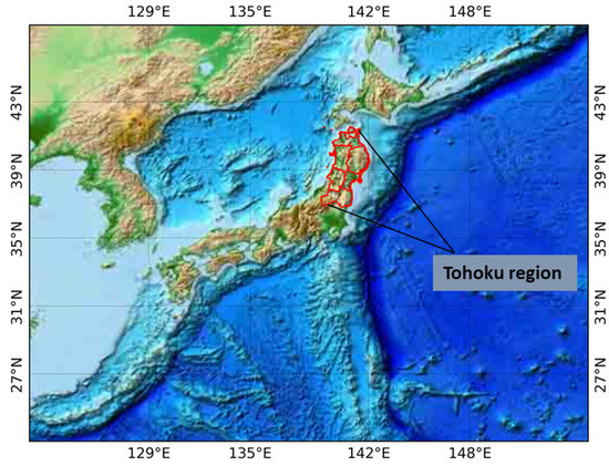
Figure 1.
Location of the study area (Tohoku region of Japan) shown by red polygons over the topographic map.
2.2. Enumeration of Dominant Plants
In Japan, plant communities have been surveyed at a national scale based on phytosociological units. With reference to existing field survey data, 126 dominant plant species were enumerated in the study area as shown in Table 1.

Table 1.
List of the dominant plant species of the Tohoku region enumerated in the research.
Geolocations (longitudes and latitudes) of the dominant species were prepared with reference to existing survey data, visual interpretation of time-lapse images available in Google Earth, and confirmation with field observations. For each dominant species, 30–90 sample points were collected as the ground truth data from a homogenous area of at least 30 × 30 m and were distributed throughout the study area. The distribution of the ground truth data in the Tohoku region is shown in Figure 2.
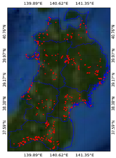
Figure 2.
Distribution of the ground truth data (red points) in the Tohoku region (blue polygon).
2.3. Genus-Physiognomy-Ecosystem (GPE) System
On the basis of field observations in different locations in the Tohoku region, the Genus-Physiognomy-Ecosystem (GPE) system has been conceived by introducing the genus and physiognomy/ecosystem inferences on the dominant species. The GPE is an intermediate level between the physiognomy/ecosystem and the dominant species for organizing plant communities. The GPE system is more detailed than the physiognomy/ecosystem level but simpler and more practical than the dominant species level. Table 2 describes the implementation of genus and physiognomy/ecosystem inferences on the dominant species.
Table 2.
Implementation of genus and physiognomy/ecosystem inferences on the dominant species.
Still, the GPE system is capable of distinguishing a wider variety of plant (ecological) communities, such as Quercus Evergreen Broadleaf Forest (EBF) (subtropical to warm temperate), Quercus Deciduous Broadleaf Forest (DBF) (cool temperate), and Quercus Shrub (alpine). Furthermore, the GPE system offers several benefits over the dominant species system. For example, the same Quercus crispula in the dominant species system can be organized into two different communities (Quercus DBF and Quercus Shrub) under the GPE system. The Quercus Shrub, namely Miyamanara (in Japanese), is a noticeable shrub community in the alpine region.
The GPE system included all dominant tree genera (deciduous/evergreen and conifer/broadleaf). However, only shrub and herbaceous genera, prominent in large patches, were organized separately, such as Rhododendron Shrub and Miscanthus Herb. It seems complicated to identify prominent patches of all shrub and herbaceous genera and more difficult to discriminate them from the satellite images. Therefore, shrub and herbaceous communities were mostly organized with physiognomy/ecosystem inferences rather than the genus inference. Interestingly, physiognomy/ecosystem inferences are more relevant to the shrub and herbaceous communities from the viewpoint of ecological and conservation significance, such as Wetland Herb and Alpine Herb.
2.4. Processing of Landsat 8 Data
Landsat 8 data offer optical imagery in visible, near infrared, and shortwave and thermal infrared wavelengths. Standard terrain corrected (Level 1T) Landsat 8 Operational Land Imager (OLI) and Thermal Infrared Sensor (TIRS) scenes available from 2017 to 2019 over the Tohoku region of Japan were utilized. The Digital Numbers (DNs) delivered as 16-bit unsigned integers were calibrated into Top-Of-Atmosphere (TOA) spectral reflectance and brightness temperature (K) values for the OLI and TIRS respectively using the rescaling coefficients available in the metadata file. The clouds were removed by using separate Quality Assessment (QA) band information. Seven spectral bands (blue, green, red, near infrared, mid infrared, shortwave infrared, and thermal infrared) were extracted. The spectral bands were composited by calculating monthly median values pixel by pixel. In this way, 84 features (12 months × 7 bands) were generated for machine learning and classification.
2.5. Machine Learning and Cross-Validation
The potential of satellite remote sensing data for the classification of plant communities at three hierarchical levels—(i) physiognomy, (ii) Genus-Physiognomy-Ecosystem (GPE), and (iii) dominant species—was evaluated by employing a machine learning technique. The pixel values, corresponding to the ground truth (geolocation points) data, were extracted for the dominant species organization of plant communities. The ground truth data were merged for other organizations of plant communities. The number of ground truth data available for dominant species organization varied from 30 to 90 for each class. However, much larger numbers of ground truth data were available for the classification at higher levels (physiognomy and GPE) because they were supersets of the lower levels. The random forests classifier was employed for the classification of satellite images with the support of ground truth data. The classification performance was assessed by utilizing a 10-fold cross-validation method. The parameters of the model were fine-tuned with reference to the cross-validation accuracy. Accuracy metrics such as kappa coefficient and f1-score were utilized for the quantitative evaluation.
3. Results
3.1. Classification at Physiognomy Level
The confusion matrix computed with the 10-fold cross-validation approach is shown in Figure 3. The classification of plant communities at the physiognomy level showed higher accuracy in terms of the kappa coefficient (0.834) and f1-score (0.879).
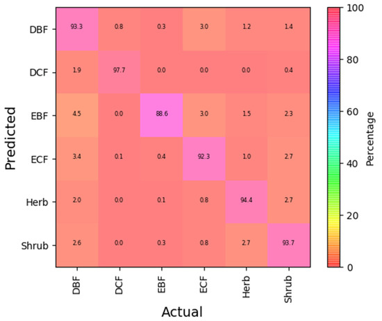
Figure 3.
Confusion matrix of the physiognomy level classification of plant communities.
The class-wise accuracy of the physiognomy level classification of plant communities is summarized in Table 3. For the class-wise accuracy, the kappa coefficients varied from 0.613 to 0.912, and the f1-scores varied from 0.615 to 0.904.
Table 3.
Class-wise performance of the physiognomy level classification of plant communities.
3.2. Classification at Dominant Species Level
The classification of dominant species (126 classes) with the 10-fold cross-validation approach showed both a kappa coefficient and f1-score of 0.820. The overall accuracy is slightly lower than the physiognomy level classification. However, the class-wise accuracy analysis (Table 4) showed poor performance of the dominant species level classification for many dominant plants. Out of 126 dominant species, 45 species showed accuracy (kappa) lower than 80%, while nine species showed accuracy (kappa) lower than 60%. The classification of plant communities at the dominant species level introduced many misclassifications and undermined its application for the operational mapping of plant communities.
Table 4.
Class-wise performance of dominant species level classification of plant communities. The numerical classes (1–126) correspond to the list of plant species enumerated and shown in Table 1.
3.3. Classification at GPE Level
Table 5 shows the class-wise performance of the Genus-Physiognomy-Ecosystem (GPE) classes introduced in the research. Besides two classes (Pterocarya DBF and Carex Herb), at least 71% accuracy (kappa) was obtained for all GPE classes. Moreover, only five classes among 51 GPE classes showed accuracy (kappa) lower than 80%. The overall accuracy (kappa = 0.872; f1-score = 0.877) was also higher than that of dominant species level classification (kappa = 0.820; f1-score = 0.820).
Table 5.
Class-wise performance of GPE level classification of plant communities.
Among the classification of six Acer species (Table 4, rows 5–10), only three species were classified with more than 80% accuracy, whereas the accuracy was very low (ranging from 0.370 to 0.747) for the other three species. These Acer species exhibit similar phenology and are difficult to discriminate separately from the spectral reflectance. When they are merged by the inference of common genus, an accuracy of 0.891 was achieved for Acer DBF (Table 5, row 2). A similar trend was obtained in almost all cases. The class-wise performance sounds important for operational mapping. The merging of similar species by the inference of genus also improved the classification of other genera with single species. For example, the average classification performance of Juglans mandshurica and Fraxinus mandshurica (Table 4) was 0.748, whereas Juglans DBF and Fraxinus DBF (Table 5) showed an average performance of 0.83.
4. Discussion
The collection of ground truth data for the supervised classification of dominant plant species is time-consuming and expensive. Plant species are mixed at the community level and finding a homogenous community of dominant species for use as the ground truth data is difficult. On the other hand, classification accuracy generally reduces with the large number of similar classes involved. Given the satellite features, the merging of similar classes can improve the performance, while the machine learning classifier cannot discern similar classes. To lessen the complexities associated with the mapping of plant communities at the dominant species level, the Genus-Physiognomy-Ecosystem (GPE) system was conceived in the research to organize the plant communities according to genus and physiognomy/ecosystem inferences.
Satellite remote sensing deals with the spectral reflectance obtained from the whole land surface, which is composed of vegetative, non-vegetative, topographic, and climatic characteristics. It should be easier to discriminate between two similar species (for example, Fagus crenata and Fagus japonica) located in different places rather than similar species located nearby, as satellite-based signals are also affected by topographic and climatic variations. Therefore, higher classification accuracies of plant communities obtained in the research might not be met during operation mapping, which has to deal with the discrimination of nearby pixels. Moreover, operational mapping involves the application of the machine learning model tuned with the given set of ground truth data to unseen new data, which may reduce the performance further.
It should be noted that the purpose of this research was not merely to extract (merge) similar classes/species as dictated by higher (lower) performance of machine learning classifiers. The overarching purpose of vegetation mapping is to discover the extent and distribution of plant communities within a geographical area of interest to meet conservation and management goals. Therefore, the GPE system involves the organization of plant communities according to ecological and conservation significance by introducing appropriate genus and physiognomy/ecosystem inferences. However, it is a flexible system in that the classes can be increased further in the future by expanding/shrinking genus/ecosystem inferences when the characteristics (spatial, spectral, and temporal resolutions) of satellite imagery and machine learning techniques advance along with the capability of improved classification and mapping. Nationwide mapping of plant communities on the basis of the GPE system is our plan for the immediate future.
5. Conclusions
This research evaluated the potential of satellite remote sensing data for the classification of plant communities at three hierarchical levels (physiognomy, Genus-Physiognomy-Ecosystem, and dominant species). The classification of 126 dominant plant species with multi-temporal satellite data in the Tohoku region of Japan showed that 45 dominant species could not be classified with accuracy (kappa) higher than 80%, while nine dominant species showed accuracy (kappa) lower than 60%. However, the GPE organization of plant communities, newly introduced in the research, showed that at least 71% accuracy (kappa) was obtained for all GPE classes besides two classes, while only 5 out of 51 classes showed accuracy (kappa) lower than 80%. The overall accuracy (kappa = 0.872; f1-score = 0.877) was also higher than that of the dominant species level classification (kappa = 0.820; f1-score = 0.820). The GPE system therefore provides a practical and easy-to-understand approach for the operational mapping and monitoring of plant communities, particularly on a broad scale.
Funding
This research was conducted with the Japan Society for the Promotion of Science (JSPS) Research Fellowship. Preparation of the ground truth data was supported by commissioned research of the Ministry of the Environment, Centre for Biodiversity and Asia Air Survey Co., Ltd. (Sarawak, Malaysia). The research was also partially supported by JSPS KAKENHI (Grant-in-Aid for Scientific Research) JP19H04320.
Institutional Review Board Statement
Not applicable.
Informed Consent Statement
Not applicable.
Data Availability Statement
Not applicable.
Acknowledgments
Keitarou Hara is greatly appreciated for invaluable advices and supports provided during the research. The Landsat 8 data were available from the United States Geological Survey (USGS). The author is thankful to the anonymous reviewers and the editors of the journal for their constructive comments.
Conflicts of Interest
The author declares no conflict of interest.
References
- Klanderud, K.; Vandvik, V.; Goldberg, D. The Importance of Biotic vs. Abiotic Drivers of Local Plant Community Composition Along Regional Bioclimatic Gradients. PLoS ONE 2015, 10, e0130205. [Google Scholar] [CrossRef] [PubMed]
- Trivellone, V.; Bougeard, S.; Giavi, S.; Krebs, P.; Balseiro, D.; Dray, S.; Moretti, M. Factors shaping community assemblages and species co-occurrence of different trophic levels. Ecol. Evol. 2017, 7, 4745–4754. [Google Scholar] [CrossRef]
- Mitchell, R.M.; Bakker, J.D.; Vincent, J.B.; Davies, G.M. Relative importance of abiotic, biotic, and disturbance drivers of plant community structure in the sagebrush steppe. Ecol. Appl. 2017, 27, 756–768. [Google Scholar] [CrossRef] [PubMed]
- Aggemyr, E.; Cousins, S.A.O. Landscape structure and land use history influence changes in island plant composition after 100 years: Revisiting 27 islands after 100 years. J. Biogeogr. 2012, 39, 1645–1656. [Google Scholar] [CrossRef]
- Rodríguez-Echeverry, J.; Echeverría, C.; Oyarzún, C.; Morales, L. Impact of land-use change on biodiversity and ecosystem services in the Chilean temperate forests. Landsc. Ecol. 2018, 33, 439–453. [Google Scholar] [CrossRef]
- Oliver, T.H.; Morecroft, M.D. Interactions between climate change and land use change on biodiversity: Attribution problems, risks, and opportunities: Interactions between climate change and land use change. Wiley Interdiscip. Rev. Clim. Chang. 2014, 5, 317–335. [Google Scholar] [CrossRef]
- Guo, F.; Lenoir, J.; Bonebrake, T.C. Land-use change interacts with climate to determine elevational species redistribution. Nat. Commun. 2018, 9, 1315. [Google Scholar] [CrossRef] [PubMed]
- Miyawaki, A.; Fujiwara, K. Vegetation Mapping in Japan. In Vegetation Mapping; Küchler, A.W., Zonneveld, I.S., Eds.; Springer: Dordrecht, The Netherlands, 1988; pp. 427–441. [Google Scholar] [CrossRef]
- Fanelli, F.; Bianco, M.; D’Angeli, D.; De Sanctis, M.; Sauli, A.S.; Testi, A.; Pignatti, S. Remote sensing in phytosociology: The map of vegetation of the Provincia of Rome. Ann. Bot. 2005, 5, 173–184. [Google Scholar]
- Xie, Y.; Sha, Z.; Yu, M. Remote sensing imagery in vegetation mapping: A review. J. Plant Ecol. 2008, 1, 9–23. [Google Scholar] [CrossRef]
- Chiarucci, A.; Araújo, M.B.; Decocq, G.; Beierkuhnlein, C.; Fernández-Palacios, J.M. The concept of potential natural vegetation: An epitaph? J. Veg. Sci. 2010, 21, 1172–1178. [Google Scholar] [CrossRef]
- Levavasseur, G.; Vrac, M.; Roche, D.M.; Paillard, D. Statistical modelling of a new global potential vegetation distribution. Environ. Res. Lett. 2012, 7, 044019. [Google Scholar] [CrossRef]
- Hengl, T.; Walsh, M.G.; Sanderman, J.; Wheeler, I.; Harrison, S.P.; Prentice, I.C. Global mapping of potential natural vegetation: An assessment of machine learning algorithms for estimating land potential. PeerJ 2018, 6, e5457. [Google Scholar] [CrossRef]
- Johansen, K.; Coops, N.C.; Gergel, S.E.; Stange, Y. Application of high spatial resolution satellite imagery for riparian and forest ecosystem classification. Remote Sens. Environ. 2007, 110, 29–44. [Google Scholar] [CrossRef]
- Meroni, M.; Ng, W.; Rembold, F.; Leonardi, U.; Atzberger, C.; Gadain, H.; Shaiye, M. Mapping Prosopis juliflora in West Somaliland with Landsat 8 Satellite Imagery and Ground Information. Land Degrad. Dev. 2017, 28, 494–506. [Google Scholar] [CrossRef]
- Wang, D.; Wan, B.; Qiu, P.; Su, Y.; Guo, Q.; Wang, R.; Sun, F.; Wu, X. Evaluating the Performance of Sentinel-2, Landsat 8 and Pléiades-1 in Mapping Mangrove Extent and Species. Remote Sens. 2018, 10, 1468. [Google Scholar] [CrossRef]
- Burai, P.; Deák, B.; Valkó, O.; Tomor, T. Classification of Herbaceous Vegetation Using Airborne Hyperspectral Imagery. Remote Sens. 2015, 7, 2046–2066. [Google Scholar] [CrossRef]
- Fu, B.; Wang, Y.; Campbell, A.; Li, Y.; Zhang, B.; Yin, S.; Xing, Z.; Jin, X. Comparison of object-based and pixel-based Random Forest algorithm for wetland vegetation mapping using high spatial resolution GF-1 and SAR data. Ecol. Indic. 2017, 73, 105–117. [Google Scholar] [CrossRef]
- Langford, Z.L.; Kumar, J.; Hoffman, F.M.; Breen, A.L.; Iversen, C.M. Arctic Vegetation Mapping Using Unsupervised Training Datasets and Convolutional Neural Networks. Remote Sens. 2019, 11, 69. [Google Scholar] [CrossRef]
- Adagbasa, E.G.; Adelabu, S.A.; Okello, T.W. Application of deep learning with stratified K-fold for vegetation species discrimation in a protected mountainous region using Sentinel-2 image. Geocarto Int. 2019, 1–21. [Google Scholar] [CrossRef]
- Tuxen, R. Die huetige potentielle naturliche Vegetation als Gegestand der Vegetationskarierung. Angew. Pflanz. 1956, 13, 5–42. [Google Scholar]
- Sharma, R.C.; Hara, K.; Tateishi, R. High-Resolution Vegetation Mapping in Japan by Combining Sentinel-2 and Landsat 8 Based Multi-Temporal Datasets through Machine Learning and Cross-Validation Approach. Land 2017, 6, 50. [Google Scholar] [CrossRef]
- Dobremez, J. Le Népal Ecologie et Biogeography; Editions du Centre National de la Recherche Scientifique: Paris, France, 1976. [Google Scholar]
- Ohsawa, M.; Shakya, P.R.; Numata, M. Distribution and Succession of West Himalayan Forest Types in the Eastern Part of the Nepal Himalaya. Mt. Res. Dev. 1986, 6, 143. [Google Scholar] [CrossRef]
- Gianguzzi, L.; Papini, F.; Cusimano, D. Phytosociological survey vegetation map of Sicily (Mediterranean region). J. Maps 2016, 12, 845–851. [Google Scholar] [CrossRef]
- Köppen, W. Das geographische System der Klimate, Handbuch der Klimatologie; Band, I., Teil, C., Eds.; Gebruder Borntraeger: Berlin, Germany, 1936; p. 46. [Google Scholar]
- Metzger, M.J.; Bunce, R.G.H.; Jongman, R.H.G.; Sayre, R.; Trabucco, A.; Zomer, R. A high-resolution bioclimate map of the world: A unifying framework for global biodiversity research and monitoring: High-resolution bioclimate map of the world. Glob. Ecol. Biogeogr. 2013, 22, 630–638. [Google Scholar] [CrossRef]
- Bailey, R.G. Ecosystem Geography: From Ecoregions to Sites; Springer: New York, NY, USA, 2009. [Google Scholar]
- Küchler, A.W. A physiognomic classification of vegetation. Ann. Assoc. Am. Geogr. 1949, 39, 201–210. [Google Scholar] [CrossRef]
- Beard, J.S. The Physiognomic Approach. In Classification of Plant Communities; Whittaker, R.H., Ed.; Springer: Dordrecht, The Netherlands, 1978; pp. 33–64. [Google Scholar]
- Grossman, D.; Faber-Langendoen, D.; Weakley, A.; Anderson, M.; Bourgeron, P.; Crawford, R.; Goodin, K.; Landaal, S.; Metzler, K.; Patterson, K. International Classification of Ecological Communities: Terrestrial Vegetation of the United States; The Nature Conservancy: Arlington, VA, USA, 1998. [Google Scholar]
- Dengler, J. Phytosociology. In International Encyclopedia of Geography: People, the Earth, Environment and Technology; Richardson, D., Castree, N., Goodchild, M.F., Kobayashi, A., Liu, W., Marston, R.A., Eds.; John Wiley & Sons, Ltd.: Oxford, UK, 2017; pp. 1–6. [Google Scholar] [CrossRef]
- Whittaker, R.H. Evolution and measurement of species diversity. Taxon 1972, 21, 213–251. [Google Scholar] [CrossRef]


Publisher’s Note: MDPI stays neutral with regard to jurisdictional claims in published maps and institutional affiliations. |
© 2021 by the author. Licensee MDPI, Basel, Switzerland. This article is an open access article distributed under the terms and conditions of the Creative Commons Attribution (CC BY) license (https://creativecommons.org/licenses/by/4.0/).