Seismically Isolating a Structure: A Rational Approach for Feasibility Assessment and Definition of Basic Parameters

Abstract

Although conceptually simple, the application of seismic isolation can pose dangerous pitfalls. It is based on decoupling the dynamic response of a structure from the ground motion by inserting isolation devices at its base. Significant displacements of the devices are typically required in return for increasing the oscillation period and reducing seismic accelerations in the building. To avoid blind guessing, the suitable values for damping and the period of vibration should be defined. The vibration period can vary in a range that depends on the capacity of the superstructure, which influences the maximum allowable acceleration, and the boundary conditions, which limit the maximum allowable displacement. In this regard, a simple and effective procedure is proposed for assessing the feasibility of seismic isolation and providing a preliminary yet reliable evaluation of the basic parameters, such as damping and the isolation period. This procedure could also highlight the need for changing the seismic protection strategy. Some application examples, aimed at including a wide range of design cases, are also provided.

1. Introduction

Seismic isolation increases the fundamental period of vibration, thereby significantly reducing the seismic action that affects the superstructure. This remains in the elastic range, preserving the construction and its content [1,2]. The numerous applications in Italy and around the world have demonstrated that seismic isolation is one of the most effective strategies for protecting structures against earthquakes [3,4,5,6,7,8,9,10].

The concept of decoupling the motion of the structure from the motion of the ground was already known in antiquity [11,12]. However, the very first isolation device appeared only in 1868, when Stevenson proposed a system with spherical rollers in niches to protect lighting systems in Japan [13]. This so-called “aseismatic joint” had the same operating principle as the modern curved surface sliders. In 1870, Touaillon proposed a similar conceptual system of spherical rollers in niches between the superstructure and the foundations [14,15]. The elliptical geometry of the housing system guaranteed the return to the initial position.

A few years later, in 1909, Mario Viscardini designed a new isolation system based on spherical rollers in niches to be used in the reconstruction of Messina and Reggio Calabria following the devastating earthquake of 1908 [16]. The new concepts seemed ready for wide use. Still, the Italian Royal Commission, established to provide advice on reconstruction, deemed it unsuitable for large-scale implementation, even if it was considered a valid alternative. Therefore, traditional techniques were used, confirming confidence in Vitruvius’ concept of firmitas, and the new ideas were abandoned.

In 1963, unreinforced rubber bearings were first used for the reconstruction of a school building in Skopje, Macedonia [17]. Excessive displacement of the devices and an undesired pitch were observed during earthquakes. Finally, rubber–steel devices were developed and realized in England in the early 1970s.

Several studies have demonstrated the convenience of seismic isolation, even considering the construction cost alone, for both reinforced concrete and masonry buildings [18,19]. The widespread adoption of seismic isolation is also linked to the availability of reliable procedures for the optimal design when the vibration period has been selected [20,21].

The design of isolation systems conceals some insides that can affect their effectiveness, both in the case of near-fault earthquakes [22] and far-fault ones. With reference to the latest, it is worth reminding that while the effectiveness of HDRB systems has been demonstrated also under low-energy earthquakes, even with significant changes in the resonance frequencies [23,24], the influence of friction on the onset of motion has been pointed out for CSS isolation systems [25,26] as well as for HDRB + SD isolation systems [27]. The effective behavior of these devices was analyzed during low-energy earthquakes, underling the importance of selecting a suitable friction value to enable the onset of motion of the devices, also during low-energy earthquakes [28,29].

These issues must be taken into account in both new constructions [30] and the retrofit of existing ones [31,32]. Therefore, a definition of a simple, reliable, easily understandable, and verifiable design procedure is essential to reduce the costs and promote the adoption of seismic isolation to mitigate seismic actions.

In this article, a rational approach to the practical application of seismic isolation in structures is proposed. A simple procedure for assessing the feasibility of seismic isolation is provided, along with criteria for selecting the isolation damping factor ξ_is and period T_is. Some examples illustrate the various cases that can occur and validate the effectiveness of the proposed procedure. This work represents a fundamental step in the optimization analysis of a seismic isolation system and, therefore, in the selection of the most suitable type of device.

2. Preliminary Considerations

Consider the recommended type 1 acceleration elastic spectrum, as defined in Eurocode 8 [33]. This assumption does not affect the validity of the study. The spectrum is defined in the range [0, 4.0 s] of the period (Figure 1). The four intervals are individualized by the period values T_B and T_C, both of which depend on the soil type, and T_D = 2.0 s. The spectrum is characterized by its maximum value for a damping ratio ξ = 0.05:

$$S_{e,\max }=a_{g}S{F}_0$$

(1)

where a_g = maximum horizontal acceleration on rigid soil (type A), F₀ = maximum spectral amplification factor, and S = soil factor, relative to the range [T_B, T_C], while in the intervals of interest for seismic isolation, the relations are:

$$\begin{gathered} S_e(T)=S_{e,\max }{\displaystyle \frac{T_C}{T}} \mathrm{for} T_C<T<T_D \\ {S}_e(T)=S_{e,\max }{\displaystyle \frac{T_C{T}_D}{T^2}} \mathrm{for} T\ge T_D \end{gathered}$$

(2)

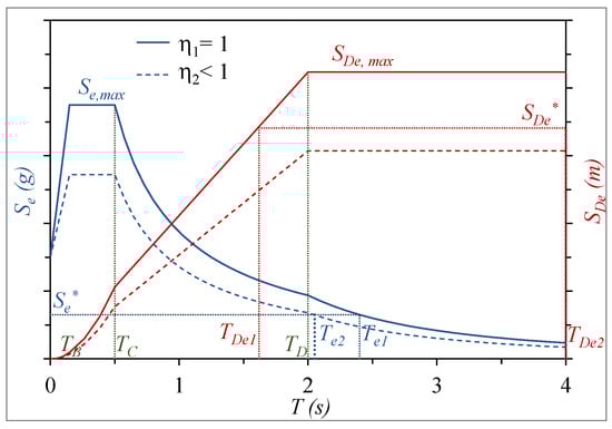
Figure 1. Elastic acceleration (blue lines) and displacement (red lines) response spectra for two values of damping, η₁ = 1 (solid lines) and η₂ < 1 (dashed lines).

For values of damping higher than 0.05, Equations (1) and (2) must be multiplied by a coefficient η, related to the damping ratio ξ by the relation $\eta =\sqrt{10/\left(5+\xi \cdot 100\right)}$. This relation is valid in the range [η_min, 1], where η_min = 0.55 (i.e., ξ_max = 0.28) according to Eurocode 8. Furthermore, for seismic isolation, a maximum value η_max is usually suggested to reduce the dynamic response in both terms of acceleration and displacement. A suitable value is η_max = 0.816, which corresponds to a minimum value of the damping factor ξ_min = 0.10. Although it is not a limit imposed by codes, it will be used in the examples illustrated in this paper.

The elastic displacement spectrum, in the same range of the period [0, 4.0 s], is obtained from the acceleration elastic spectrum S_e, dividing it by the square of pulsation and amplifying it by the factor γ_x = 1.2, which accounts for the particular importance of the devices in seismically isolated structures:

$$S_{De}(T)={\gamma }_x{S}_e\cdot {\left(T/2\pi \right)}^2$$

(3)

It reaches its maximum constant value for T ≥ T_D and depends on the soil type through T_C:

$$S_{De,\max }={\gamma }_x{S}_{e,\max }\cdot T_C{T}_D/{\left(2\pi \right)}^2$$

(4)

The design of a seismic isolation system is dictated by the need to reduce the acceleration in the superstructure while simultaneously limiting the maximum displacement of the isolation devices. Therefore, the following spectral thresholds must be fixed (Figure 1):

• The highest allowed value of the spectrum acceleration $S_e^{\ast }$: It is related to the maximum seismic action that the superstructure can withstand within the elastic range and is chosen based on economic considerations or a vulnerability analysis in the case of existing structures. $S_e^{\ast }$ corresponds to a value T_e of the period in the spectrum.
• The highest allowed value of the spectrum displacement $S_{De}^{\ast }$: It is related to the maximum seismic displacement $d_E^{\ast }$ consistent with the boundary conditions. $S_{De}^{\ast }$ corresponds to a value T_De of the period in the spectrum.

Both the previous maximum acceleration and displacement values are fixed considering that these are the effects of the main seismic component. These effects must be added to those of the horizontal orthogonal component and, when requested, of the vertical one. According to Eurocode 8, both the horizontal orthogonal and vertical components are reduced to 30% of their characteristic values.

A suitable value of the isolation period T_is must respect the relation:

$$T_e\le T_{is}\le T_{De}$$

(5)

Therefore, it must be T_e ≤ T_De. This is guaranteed only for values of the damping ξ_is higher than a specific value.

The problem simplifies when considering that the spectral displacement remains constant for a period higher than T_D = 2.0 s. Furthermore, it is usually assumed that T_is ≥ 2.0 s to obtain a significant reduction in seismic action, as well as a suitable dynamic decoupling between the superstructure and the substructure. Therefore, if the maximum spectral displacement $S_{De}(T_D)$ is not higher than the threshold value $S_{De}^{\ast }$, the condition on the displacement is certainly satisfied, and T_De is not defined. In this case, any value of T_e in the spectrum validity range can be accepted, and T_is ≥ T_e. The need for more accurate evaluations comes when the space around the building is limited and the highest allowed value of displacement requires an isolation period T_is < T_D.

Given the above, a procedure is proposed in the following section, which enables the establishment, in a preliminary feasibility analysis, of whether the isolation strategy is feasible and effective according to the specific design conditions and allows for selecting the basic design parameters, i.e., the damping factor and isolation period.

3. Characteristic Values for Damping

The damping value must be defined to satisfy the requirements concerning the maximum admissible acceleration in the superstructure and the maximum displacement consistent with the boundary conditions. The sections below analyze the ranges within which the damping value can be selected, depending on the region of the elastic response spectrum being considered.

3.1. The Characteristic Value η′

From the condition $S_{De}(T_D)\le S_{De}^{\ast }$, the following upper bound for η_is (i.e., a lower bound for ξ_is) can be deduced, which depends on the spectral displacement $S_{De}^{\ast }/S_{De,\max }$ only:

$${\eta }^{\prime }={\displaystyle \frac{S_{De}^{\ast }}{S_{De,\max }}}={\displaystyle \frac{{\left(2\pi \right)}^2}{S_{e,\max }{T}_C{T}_D}}{\displaystyle \frac{S_{De}^{\ast }}{{\gamma }_x}}$$

(6)

If η′ ≥ η_min (i.e., the corresponding damping factor ξ′ ≤ ξ_max), then a suitable value η_is in the range [η_min, η′] can be chosen.

When η_is has been fixed, the period T_e can subsequently be determined using one of the two following relations:

$$\begin{gathered} T_e={\displaystyle \frac{S_{e,\max }{T}_C}{S_e^{\ast }}}{\eta }_{is} \mathrm{if} T_e<T_D \\ {T}_e=\sqrt{{\displaystyle \frac{S_{e,\max }{T}_C{T}_D}{S_e^{\ast }}}{\eta }_{is}} \mathrm{if} T_e\ge T_D \end{gathered}$$

(7)

At this point, any value T_is ≥ T_e can be assumed for the isolation period without any restrictions due to T_De.

3.2. The Characteristic Value η″

If η′ < η_min (i.e., ξ′ > ξ_max), the relation $S_{De}(T_D)\le S_{De}^{\ast }$ cannot be satisfied. Therefore, a suitable value of the isolation period T_is must be searched in the range [T_C, T_D[, where the relations for T_e and T_De are, respectively:

$$T_e={\displaystyle \frac{S_{e,\max }{T}_C}{S_e^{\ast }}}\eta T_{De}={\displaystyle \frac{{\left(2\pi \right)}^2}{S_{e,\max }{T}_C}}{\displaystyle \frac{S_{De}^{\ast }}{{\gamma }_x}}{\displaystyle \frac{1}{\eta }}$$

(8)

The condition T_e ≤ T_De gives a new upper bound for η_is, which also depends on the spectral acceleration $S_e^{\ast }/S_{e,\max }^{\ast }$:

$${\eta }^{″}=\sqrt{{\displaystyle \frac{S_e^{\ast }}{S_{e,\max }}}{\displaystyle \frac{S_{De}^{\ast }}{S_{De,\max }}}{\displaystyle \frac{T_D}{T_C}}}={\displaystyle \frac{\left(2\pi \right)}{S_{e,\max }{T}_C}}\sqrt{S_e^{\ast }{\displaystyle \frac{S_{De}^{\ast }}{{\gamma }_x}}}$$

(9)

If η″ > η_min, then any value η_is in the range [η_min, η″] can be assumed, and an isolation period T_is between T_e and T_De, corresponding to η_is, can be freely set.

If both η′ and η″ are lower than the minimum value η_min, then one or both of the thresholds $S_e^{\ast }$ and $S_{De}^{\ast }$ must be modified. As a last resort, the isolation strategy is not pursuable.

4. Procedure to Rationally Approach a Seismic Isolation Design

4.1. Feasibility Assessment

Setting η′ ≥ η_min in Equation (6) and η″ > η_min in Equation (9), the following inequalities are obtained, respectively, in which $S_{De}^{\ast }$ is expressed as a function of $S_e^{\ast }$ in non-dimensional form (with respect to the $S_{e,\max }$ and $S_{De,\max }$, respectively, obtained for η = 1):

$${\displaystyle \frac{S_{De}^{\ast }}{S_{De,\max }}}\ge {\eta }_{\min } {\displaystyle \frac{S_{De}^{\ast }}{S_{De,\max }}}\ge {\displaystyle \frac{{\left({\eta }_{\min }\right)}^2}{S_e^{\ast }/S_{e,\max }}}{\displaystyle \frac{T_C}{T_D}}$$

(10)

The curves corresponding to the two equalities are plotted in Figure 2 (continuous lines) and represent a lower boundary for the admissible couples of values ( $S_{De}^{\ast }$, $S_e^{\ast }$). It is worth noting that the first Equation (10) gives a constant value equal to η_min, while the second depends on T_C, i.e., on the soil type (A, B, C, or D, according to the Eurocode 8 definitions). The diagrams are dimensionless with respect to the seismicity of the area, which, therefore, does not affect them.

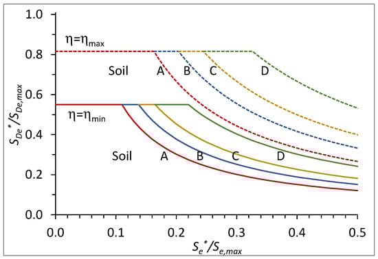
Figure 2. $S_{De}^{\ast }$ as a function of $S_e^{\ast }$ in non-dimensional forms for η = η_min (solid lines) and η = η_max (dashed lines).

The curves relative to η_max are also plotted in the same figure (dotted lines). Each pair of curves relative to the same soil type individualizes a feasibility area, i.e., a portion of the plane of admissible values for the couples $S_e^{\ast }$ and $S_{De}^{\ast }$.

If the couple of values ( $S_e^{\ast }$, $S_{De}^{\ast }$) corresponds to a non-admissible point, one or both thresholds should be increased. The diagram helps identify the closest solution to be achieved, for example, by what ratio the threshold values should be increased. It allows for determining whether the isolation strategy is feasible.

Once it has been established that the isolation strategy is feasible, the next step involves designing the basic parameters, specifically the damping ratio and the isolation period.

4.2. Choosing Damping Ratio and Isolation Period

Suppose that the elastic spectra at the site for η = 1 are known and the fixed spectral thresholds $S_e^{\ast }$ and $S_{De}^{\ast }$ correspond to an admissible point. Then, the choice of T_is is oriented at obtaining the following:

• A spectral acceleration $S_e(T_{is})\le S_e^{\ast }$, which guarantees a suitable reduction of the seismic action in the superstructure.
• A spectral displacement $S_{De}(T_{is})\le S_{De}^{\ast }$ (the displacement spectrum being amplified by γ_x) for which the value reached for seismic displacement d_E under the design seismic actions is not higher than the allowed one $d_E^{\ast }$. In the absence of other effects, it can be assumed that $d_E=S_{De}^{\ast }\sqrt{1+{0.3}^2}\approx 1.05\cdot S_{De}^{\ast }$.

In addition to the previously discussed constraints on T_is, it is necessary to consider that the isolation period should be at least three times the vibration period T_fb of the superstructure supposedly fixed at its base to achieve suitable dynamic decoupling between the superstructure and the substructure.

Taking into account what has been said in the previous paragraph, once η′ and η″ have been computed, a procedure aimed at choosing ξ_is and T_is could be organized as follows.

Consider first the case in which η′ ≥ η_min (i.e., ξ′ ≤ ξ_max), shown in Figure 3a. Assume a suitable value of η_is in the range [η_min, η′] and determine the corresponding damping factor ξ_is. With T_De being indefinite and not affecting the eligibility of T_is, calculate the value of T_e and assume T_is ≥ T_e. Two situations can occur:

• If η_is = η′ and T_is ≥ T_D, then $S_{De}\left(T_{is}\right)=S_{De}^{\ast }$, and the effective total displacement d_E is equal to $d_E^{\ast }$.
• If η_is < η′ or T_is < T_D, then $S_{De}\left(T_{is}\right)<S_{De}^{\ast }$, and d_E is less than $d_E^{\ast }$.

Figure 3. Graphical description of the design cases: (a) η′ ≥ η_min; (b) η′ < η_min; (c) η″ ≥ η_min; (d) η″ < η_min. Elastic acceleration and displacement response spectra are given in blue and red lines, respectively.

If η′ < η_min (i.e., ξ′ > ξ_max), the two spectral thresholds could be incompatible with each other, as is the case in Figure 3b, whatever the value of η_is in the range [η_min, η_max]. The isolation period T_is will be searched in the range [T_C, T_D], and a check on η″ is required.

If η″ ≥ η_min (Figure 3c), assuming a value of η_is in the range [η_min, η″], a suitable T_is can be found in the range [T_e, T_De], defined by Equation (8). In more detail:

• If η_is = η″, it will be T_e = T_De < T_D. Therefore, there will be just one solution for the isolation period, i.e., T_is = T_e, corresponding to $S_e(T_{is})=S_e^{\ast }$ and $S_{De}(T_{is})=S_{De}^{\ast }$.
• If η_is < η″, it will be T_e < T_De. Suppose T_is = T_De; then, $S_{De}(T_{is})=S_{De}^{\ast }$, but $S_e(T_{is})<S_e^{\ast }$. If we assume T_is = T_e, then $S_e(T_{is})=S_e^{\ast }$, but $S_{De}(T_{is})<S_{De}^{\ast }$.

If η″ < η_min as well (Figure 3d), we would fall into the case classified as non-admissible in the feasibility check.

4.3. The Capacity Spectrum Approach

The previous considerations can be effectively represented by using the $S_e-S_{De}$ capacity spectrum (Figure 4). Consider the spectrum for η = 1 (ξ = 0.05, sky blue line), which sets the maximum spectral values $S_{e,\max }$ and $S_{De,\max }$. Then, consider the spectra for η = η_max (ξ = ξ_min, blue line) and η = η_min (ξ = ξ_max, red line). These spectra represent the higher and lower limits for the S_e–S_De pairs of values, respectively. All the spectra are characterized by their portions with constant and maximum acceleration $\eta S_{e,\max }$ and with constant and maximum displacement $\eta S_{De,\max }$, while the curve between them is relative to the maximum constant velocity $\eta S_{Ve,\max }$. The half-lines starting from the origin, relating to the periods T_C, T_D, and T = 4 s, are identified.

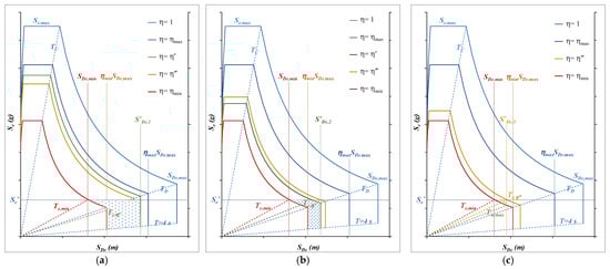
Figure 4. The three situations that can occur, analyzed in the capacity spectrum : (a) η′ > η″ > η_min, (b) η″ > η′ > η_min, and (c) η″ > η_min > η′.

Suppose the value $S_e^{\ast }$ is fixed. Three situations can occur, relative to different values of $S_{De}^{\ast }$, denoted by subscripts 1, 2, and 3, respectively. For each of them, the values of η′ and η″ can be evaluated.

In the first case ( $S_{De}^{\ast }=S_{De,1}^{\ast }$, Figure 4a), it is η′ > η″ > η_min, and an admissible value of η′ (≥ η_min) exists for which $S_{De,1}^{\ast }={\eta }^{\prime }{S}_{De,\max }$. The lines $S_e=S_e^{\ast }$ and $S_{De}=S_{De,1}^{\ast }$ define, with the spectrum η_min, the blue dotted area of the admissible pairs $S_{De}-S_e$. The spectrum η″ does not influence the result. For points in the area between lines $S_e=S_e^{\ast }$ and T = T_D and the spectrum η_min, it is T_e < T_D. For each η, T_is must be between T_e and 4 s.

In the second case ( $S_{De}^{\ast }=S_{De,2}^{\ast }$, Figure 4b), it is η″ > η′ > η_min. The lines $S_e=S_e^{\ast }$ and $S_{De}=S_{De,2}^{\ast }$ and the spectrum η′ define, with the spectrum η_min, the blue dotted area of the admissible pairs $S_{De}-S_e$. Furthermore, the spectrum η″ defines the dotted yellow area (between lines $S_e=S_e^{\ast }$ and $S_{De}=S_{De,2}^{\ast }$, the spectrum η′, and the spectrum η_min) characterized by a value of η between η′ and η″. For points in this area, it is T_e < T_D and $S_{De}<\eta S_{De,\max }$. For each η, T_is must be between T_e and 4 s.

In the third case ( $S_{De}^{\ast }=S_{De,3}^{\ast }$, Figure 4c), it is η″ > η_min > η′. The blue area does not exist. The lines $S_e=S_e^{\ast }$ and $S_{De}=S_{De,2}^{\ast }$ define, with the spectrum η_min, the yellow dotted area of the admissible pairs $S_{De}-S_e$. Points in this area belong to spectra with η between η_min and η″. The spectrum η″ passes through the point ( $S_e^{\ast }$, $S_{De,3}^{\ast }$). For points in this area, it is T_e < T_D. For each η, T_is must be between T_e and a maximum value of T < 4 s.

If $S_{De}^{\ast }<S_{De,\min }$, there is no solution. The point at which the spectrum relative to η = η_min assumes a value $S_e^{\ast }$ defines the minimum value for the period T_e.

The capacity spectrum is an optimal tool for graphically deducing the basic parameters of the isolation system, as each point uniquely identifies a damping ratio and a period. Once spectra corresponding to the relevant values of η, given above, are plotted and the space vertically and horizontally bounded through $S_e^{\ast }$ and $S_{De}^{\ast }$, respectively, the area including all possible solutions is clearly defined. This is shown through some examples in the following paragraph.

5. Examples

In the following numerical applications, the values η_min = 0.55 and η_max = 0.816 are assumed. Suppose that the maximum spectral acceleration for a site on soil type B, i.e., the value between T_C = 0.5 s and T_D = 2.0 s for ξ = 0.05, is:

$$S_{e,\max }=1.05\mathrm{g}$$

(11)

The maximum spectral displacement, which occurs for T > T_D, can be deduced:

$$S_{De,\max }=0.313\mathrm{m}$$

(12)

Consider the eight case studies summarized in Table 1, which considers two threshold values for $S_e^{\ast }$. The first, equal to 0.10 g, is often assumed in the seismic retrofit of existing structures; the second, equal to 0.20 g, can be considered as a suitable value for newly built buildings. For each of them, four threshold values for $S_{De}^{\ast }$ (150, 200, 250, and 300 mm, respectively) have been considered.

Table 1. Cases with $S_e^{\ast }$ = 0.10 g and $S_e^{\ast }$ = 0.20 g, for different values of $S_{De}^{\ast }$. Two solutions, marked as a and b, are given.

Case	1.1		1.2		1.3		1.4
$S_e^{\ast }$ (g)	0.10
$S_{De}^{\ast }$ (mm)	150		200		250		300
η′	0.479		0.639		0.798		0.958
ξ′ (%)	38.6		19.5		10.7		5.9
η″	0.427		0.493		0.552		0.604
ξ″ (%)	49.8		36.1		27.9		22.4
Solution	-	-	a	b	a	b	a	b
ξis (%)	-	-	19.5	25.0	10.7	17.0	10.0	17.0
ηis	-	-	0.639	0.577	0.798	0.674	0.816	0.674
Tis = Te (s)	-	-	2.59	2.46	2.90	2.66	2.93	2.66
Se,is (g)	-	-	0.10	0.10	0.10	0.10	0.10	0.10
SDe,is (mm)	-	-	200	181	250	211	256	211
Case	2.1		2.2		2.3		2.4
$S_e^{\ast }$(g)	0.20
$S_{De}^{\ast }$(mm)	150		200		250		300
η′	0.479		0.639		0.798		0.958
ξ′ (%)	38.6		19.5		10.7		5.9
η″	0.604		0.698		0.780		0.854
ξ″ (%)	22.4		15.5		11.4		8.7
Solution	a	b	a	b	a	b	a	b
ξis (%)	22.4	25.0	15.5	20.0	10.7	17.0	10.0	17.0
ηis	0.604	0.577	0.698	0.632	0.798	0.674	0.816	0.674
Tis = Te (s)	1.59	1.52	1.83	1.66	2.05	1.77	2.07	1.77
Se,is (g)	0.20	0.20	0.20	0.20	0.20	0.20	0.20	0.20
SDe,is (mm)	150	137	200	164	250	187	256	187

The feasibility check consists of superimposing the couples of spectral thresholds onto the plane of admissible values, as shown in Figure 5, to determine whether the isolation strategy is feasible or not. It is immediately evident that case 1.1 corresponds to a non-admissible point and requires one or both thresholds to be increased.

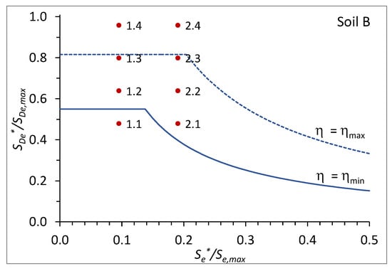
Figure 5. Feasibility check: couples of spectral thresholds superimposed on the plane of admissible values.

This can also be viewed in Table 1, where the characteristic parameters η’ and η″ and the corresponding values of the damping ratios are reported.

The considered cases cover all the possible situations that can occur. Let us analyze them with the help of the normalized capacity spectra (Figure 6), in which the values of $S_e/S_e^{\ast }$ and $S_{De}/S_{De}^{\ast }$ are reported. For each case, the capacity spectra relative to η’ and η″ are plotted in addition to those relative to η = η_min and η = η_max. The admissible values are to be searched in the area limited by the straight lines $S_e/S_e^{\ast }$ = 1, $S_{De}/S_{De}^{\ast }$ = 1, and T = 4 s and the spectrum relative to η = η_min. This area is gray colored in the figures. The bisector line represents the pairs of values ($S_e/S_e^{\ast }$ and $S_{De}/S_{De}^{\ast }$) for which T_e = T_De. The following typical situations can be distinguished:

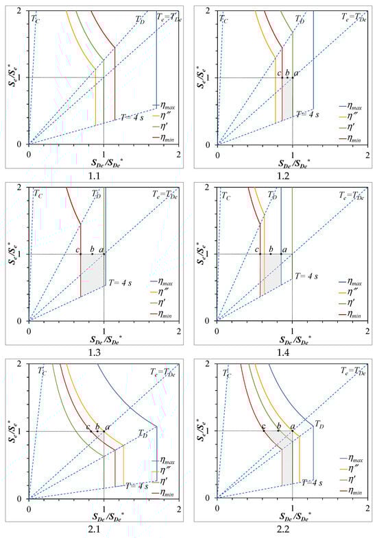
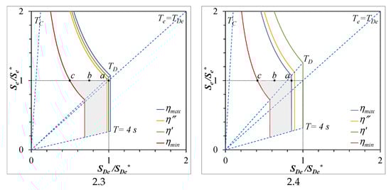
Figure 6. Normalized capacity spectra for the eight considered cases. Grey area delimits the area of admissible values for basic parameters η_is and T_is.

• In case 1.1, it is η″ < η’ < η_min, and no solutions respect the spectral thresholds, as already pointed out by the feasibility check.
• In cases 1.2, 1.3, and 2.3, it is η_min < η’ < η_max, and η″ < η’. The value of η_is can be chosen between η_min and η’.
• In cases 1.4 and 2.4, it is η_min < η_max < η’ and η″ < η’. The value of η_is can be chosen between η_min and η_max.
• In case 2.1, it is η’ < η_min < η″ <η_max. The value of η_is can be chosen between η_min and η″.
• In case 2.2, it is η_min < η’ < η″ <η_max. The value of η_is can be chosen between η_min and η″.

It is interesting to note that for low values of $S_e^{\ast }$ (cases 1.2, 1.3, and 1.4) or high values of $S_{De}^{\ast }$ (cases 2.3 and 2.4), the period T_e = T_De is greater than T_D, but T_De is in reality not limited. In these cases, the point $S_e/S_e^{\ast }=S_{De}/S_{De}^{\ast }=1$ is no longer on the spectrum of η″ but on the extrapolation of its constant velocity section to periods greater than T_D. The point $S_e/S_e^{\ast }=S_{De}/S_{De}^{\ast }=1$ will be on the spectrum of η’. In this case, it is η″ < η’.

For each case, three possible solutions have been highlighted in the figures, marked as a, b, and c, respectively. The corresponding basic parameters are reported in Table 1. All solutions respect the condition $S_e/S_e^{\ast }$ = 1, but among them, the following are true:

• Solution a represents the solution with the lower value of damping ξ_is and the highest value of T_is. Greater values of T_is can be considered as moving along a vertical straight line for a, obtaining $S_e<S_e^{\ast }$.
• Solution c is relative to η_is = η_min and corresponds to the maximum value of damping ξ_is = ξ_max. It is associated with the lowest value of T_is and $S_{De}<S_{De}^{\ast }$.
• Solution b represents an intermediate situation between the previous ones, in which it is certainly $S_{De}<S_{De}^{\ast }$.

The previous considerations influence the choice of the isolation type to use. On the other hand, the optimum solution depends on the devices used.

6. Application to Real Isolation Systems

Once T_is has been fixed, the total mass M being known with a good approximation, the total stiffness of the isolation system can be deduced:

$$k_{esi}={\left({\displaystyle \frac{2\pi }{T_{is}}}\right)}^2\cdot M$$

(13)

It is equal to the sum of the stiffness of all devices. Regarding curved surface sliders (CSSs), the stiffness varies for each isolator, even if they are all the same in terms of geometry and materials, because it depends on the mass m, i.e., on the vertical load N acting on each device.

As shown in the previous paragraph, numerous solutions can be found if remaining in the gray area, which applies regardless of the type of isolation device. The final choice in terms of damping ξ_is and period T_is will depend on the type of seismic isolator that you intend to use. Some points are summarized below.

In the case of an isolation system composed of high damping rubber bearings (HDRBs) and sliding devices (SDs), once the number of elastomeric devices has been determined, the stiffness of the individual isolator is derived from Equation (13). Taking into account the required displacement and the maximum vertical load acting on the individual device, it can be designed in compliance with the standard specifications. In this phase, the final value of the period T_is may be established to meet optimum or commercial dimensions of the diameter and thickness of the rubber.

In the case of CSSs, the values of damping and the isolation period, freely chosen within the gray area, may result in friction coefficient and equivalent radius values that are not satisfactory. Generally, it is best to fix the friction coefficient and then calculate the corresponding radius, keeping the damping constant. In this case, both the period T_is and the seismic displacement can vary. Therefore, the final solution must be sought through an iterative process.

7. Conclusions

In this paper, a methodology for preliminarily evaluating the feasibility of a seismic isolation strategy under assigned design conditions and selecting the basic parameters of the isolation system, i.e., the damping parameter η_is and the isolation period T_is, has been proposed. The design conditions are given in terms of the highest spectrum acceleration $S_e^{\ast }$, the highest spectrum displacement $S_{De}^{\ast }$, and the seismicity of the area.

The main findings can be summarized as follows:

• A feasibility area on the plane ( $S_e^{\ast }$, $S_{De}^{\ast }$) can be individualized, which allows for checking immediately if a pair of threshold values ( $S_e^{\ast }$, $S_{De}^{\ast }$) is admissible or whether one or both of them should be increased (Figure 2).
• For any admissible pair, two parameters related to damping, namely η’ and η″, can be defined based on the design conditions (Equations (6) and (9)).
• The analysis of these parameters and the comparison of them with the maximum and minimum values, η_min and η_max, allow for defining the range of admissible values for η_is and T_is.
• If η′ > η″ > η_min, a wide admissible area can be defined on the ( $S_e^{\ast }$, $S_{De}^{\ast }$) plane. A value of η between η_min and η′ and isolation periods between T_e and 4 s can be chosen.
• If η″ > η′ > η_min, values of η between η′ and η″ allow for enlarging the admissible area, but for these points, the isolation period will be lower than T_D.
• If η″ > η_min > η′, values of η between η″ and η_min can be chosen. It is T_e < T_D, and T_e must be between T_e and a maximum value of T < 4 s.
• If both η′ and η″ are lower than η_min, $S_e^{\ast }$ and $S_{De}^{\ast }$ are inconsistent with each other, and the design conditions must be changed to pursue the isolation strategy.

The proposed procedure has been tested in a few demonstrative examples, spanning a wide range of spectral thresholds $S_e^{\ast }$ and $S_{De}^{\ast }$. A graphical approach has also been provided through capacity spectra aimed at delimiting the space of solution.

The described considerations influence the final choice of the devices to be used. On the other hand, the design values and performance optimization of the system depend on the seismic device you intend to use, i.e., on additional factors also, such as material savings and simplification of the manufacturing process. These aspects will be the subjects of future developments.

References

- Naeim, F.; Kelly, J.M. Design of Seismic Isolated Structures: From Theory to Practice; John Wiley & Sons, Inc.: Hoboken, NJ, USA, 1999. [Google Scholar]
- Skinner, R.I.; Robinson, W.H.; McVerry, G.H. An Introduction to Seismic Isolation; John Wiley & Sons Ltd.: Hoboken, NJ, USA, 1993. [Google Scholar]
- Clemente, P. New Challenges in the Development and Application of Seismic Isolation. In Earthquake Resistant Design, Protection, and Performance Assessment in Earthquake Engineering, Proceedings of the AERS 2023, Baku, Azerbaijan, 26–28 April 2023; Kasimzade, A., Erdik, M., Kundu, T., Sucuoğlu, H., Clemente, P., Eds.; Geotechnical, Geological and Earthquake Engineering; Springer: Cham, Switzerland, 2024; Volume 54, pp. 44–60. [Google Scholar] [CrossRef]
- Saito, T. Learning from the Past: The Resilient Design and Performance of Seismically Isolated Buildings in Japan. In Seismic Isolation, Energy Dissipation and Active Vibration Control of Structures, Proceedings of the 18th World Conference on Seismic Isolation, Antalya, Turkey, 6–10 November 2023; Lecture Notes in Civil Engineering; Springer: Cham, Switzerland, 2024; Volume 533, pp. 255–269. [Google Scholar] [CrossRef]
- Zhou, F.; Tan, P.; Chen, Y.; Liu, Y. Recent Development and Application on Seismic Isolation, Energy Dissipation and Vibration Control in China. In Seismic Isolation, Energy Dissipation and Active Vibration Control of Structures, Proceedings of the 17th World Conference on Seismic Isolation, Turin, Italy, 11–16 September 2022; Lecture Notes in Civil Engineering; Springer: Cham, Switzerland, 2023; Volume 309, pp. 59–73. [Google Scholar] [CrossRef]
- Aiken, I.; Black, C. Recent Developments and Applications of Seismic Isolation in North America. In Seismic Isolation, Energy Dissipation and Active Vibration Control of Structures, Proceedings of the 17th World Conference on Seismic Isolation, Turin, Italy, 11–16 September 2022; Lecture Notes in Civil Engineering; Springer: Cham, Switzerland, 2023; Volume 309, pp. 74–85. [Google Scholar] [CrossRef]
- Saito, T. Efforts Toward International Harmonization of Seismic Isolation Design Code and Current Status in Japan. In Seismic Isolation, Energy Dissipation and Active Vibration Control of Structures, Proceedings of the 17th World Conference on Seismic Isolation, Turin, Italy, 11–16 September 2022; Lecture Notes in Civil Engineering; Springer: Cham, Switzerland, 2023; Volume 309, pp. 47–58. [Google Scholar] [CrossRef]
- Sadan, B. State of the Art in Application of Seismic Isolation and Energy Dissipation in Turkey. In Seismic Isolation, Energy Dissipation and Active Vibration Control of Structures, Proceedings of the 17th World Conference on Seismic Isolation, Turin, Italy, 11–16 September 2022; Lecture Notes in Civil Engineering; Springer: Cham, Switzerland, 2023; Volume 309, pp. 17–25. [Google Scholar] [CrossRef]
- Dutu, A.; Iordachescu, A.; Mocanu, D.; Soveja, L. Seismic Isolation Applications in Romania. In Seismic Isolation, Energy Dissipation and Active Vibration Control of Structures, Proceedings of the 17th World Conference on Seismic Isolation, Turin, Italy, 11–16 September 2022; Lecture Notes in Civil Engineering; Springer: Cham, Switzerland, 2023; Volume 309, pp. 26–46. [Google Scholar] [CrossRef]
- Boroschek, R.; Retamales, R. Seismic Isolation in Chile: An Opportunity for Model Codes. In Seismic Isolation, Energy Dissipation and Active Vibration Control of Structures, Proceedings of the 17th World Conference on Seismic Isolation, Turin, Italy, 11–16 September 2022; Lecture Notes in Civil Engineering; Springer: Cham, Switzerland, 2023; Volume 309, pp. 86–99. [Google Scholar] [CrossRef]
- Carpani, B. Base isolation from a historical perspective. In Proceedings of the 16th World Conference on Earthquake Engineering, Santiago, Chile, 9–13 January 2017; IAEE & ACHISINA: Santiago, Chile, 2017. [Google Scholar]
- Clemente, P. Seismic isolation: Past, present and the importance of SHM for the future. J. Civ. Struct. Health Monit. 2017, 7, 217–231. [Google Scholar] [CrossRef]
- Stevenson; Douglass; Lloyd, W.; Pole, W.; Abernethy; Woods; Beaumont; Brunton; Cay, W.D.; Coleman, J.J. Discussion. The Japan lights. Minutes Proc. Inst. Civ. Eng. 1877, 47, 26–41. [Google Scholar] [CrossRef]
- Harvey, P.S.; Kelly, K.C. A review of rolling-type seismic isolation: Historical development and future directions. Eng. Struct. 2016, 125, 521–553. [Google Scholar] [CrossRef]
- Makris, N. Seismic isolation: Early history. Earthq. Eng. Struct. Dyn. 2019, 48, 269–283. [Google Scholar] [CrossRef]
- Calvi, P.M.; Fagà, G.; Calvi, G.M. Historical development of friction-based seismic isolation systems. Progett. Sismica 2018, 10, 13–39. [Google Scholar] [CrossRef]
- Marioni, A. Early Applications of Anti-seismic Measures. In Anti-Seismic Devices; Springer: Cham, Switzerland, 2024. [Google Scholar] [CrossRef]
- Clemente, P.; Buffarini, G. Base isolation: Design and optimization criteria. J. Seism. Isol. Prot. Syst. 2010, 1, 17–40. [Google Scholar] [CrossRef]
- Clemente, P.; Bontempi, F.; Boccamazzo, A. Seismic Isolation in Masonry Buildings: Technological and economic issues. In Brick and Block Masonry: Trends, Innovation and Challenges, Proceedings of the 6th International Conference IB2MAC, Padua, Italy, 26–30 June 2016; Modena, C., da Porto, F., Valluzzi, M.R., Eds.; CRC Press: Boca Raton, FL, USA; Taylor & Francis Group: London, UK, 2016; pp. 2207–2215. [Google Scholar] [CrossRef]
- Tripepi, C.; Clemente, P. Graphic Procedure for the Optimum Design of Elastomeric Isolators. Pract. Period. Struct. Des. Constr. 2021, 26, 04020058. [Google Scholar] [CrossRef]
- Feng, D.; Saito, T.; Wu, H.; Liu, W. Seismic Isolation Design Comparison of Japan, China, USA and Eurocode. In Seismic Isolation, Energy Dissipation and Active Vibration Control of Structures, Proceedings of the 17th World Conference on Seismic Isolation, Turin, Italy, 11–16 September 2022; Lecture Notes in Civil Engineering; Springer: Cham, Switzerland, 2023; Volume 309, pp. 317–325. [Google Scholar] [CrossRef]
- Erdik, M.; Sadan, B.; Tüzün, C.; Demircioglu-Tumsa, M.B.; Ülker, Ö.; Harmandar, E. Near-Fault Earthquake Ground Motion and Seismic Isolation Design. In Seismic Isolation, Energy Dissipation and Active Vibration Control of Structures, Proceedings of the 17th World Conference on Seismic Isolation, Turin, Italy, 11–16 September 2022; Lecture Notes in Civil Engineering; Springer: Cham, Switzerland, 2023; Volume 309, pp. 117–152. [Google Scholar] [CrossRef]
- Clemente, P.; Bongiovanni, G.; Buffarini, G.; Saitta, F.; Castellano, M.G.; Scafati, F. Effectiveness of HDRB isolation systems under low energy earthquakes. Soil Dyn. Earthq. Eng. 2019, 118, 207–220. [Google Scholar] [CrossRef]
- Clemente, P.; Di Cicco, A.; Saitta, F.; Salvatori, A. Seismic Behaviour of Base Isolated Civil Protection Operative Centre in Foligno, Italy. J. Perform. Constr. Facil. 2021, 35, 04021027. [Google Scholar] [CrossRef]
- Clemente, P.; Bongiovanni, G.; Buffarini, G.; Saitta, F.; Scafati, F. Monitored Seismic Behavior of Base Isolated Buildings in Italy. In Seismic Structural Health Monitoring; Limongelli, M., Çelebi, M., Eds.; Springer Tracts in Civil Engineering; Springer: Cham, Switzerland, 2019; pp. 115–137. [Google Scholar] [CrossRef]
- Scafati, F.; Ormando, C.; Clemente, P.; Bongiovanni, G. Observed behavior of buildings seismically isolated with CSSs under a low energy earthquake. J. Civ. Struct. Health Monit. 2022, 12, 225–243. [Google Scholar] [CrossRef]
- Salvatori, A.; Bongiovanni, G.; Clemente, P.; Ormando, C.; Saitta, F.; Scafati, F. Observed seismic behaviour of a HDRB and SD isolation system under far fault earthquakes. Infrastructures 2022, 7, 13. [Google Scholar] [CrossRef]
- Gandelli, E.; Quaglini, V. Effect of the Static Coefficient of Friction of Curved Surface Sliders on the Response of an Isolated Building. J. Earthq. Eng. 2018, 24, 1361–1389. [Google Scholar] [CrossRef]
- Saitta, F.; Clemente, P.; Bongiovanni, G.; Buffarini, G.; Salvatori, A.; Grossi, C. Base isolation of buildings with curved surface sliders: Basic design criteria and critical issues. Adv. Civ. Eng. 2018, 2018, 1569683. [Google Scholar] [CrossRef]
- Clemente, P. Applications and recent studies on seismic isolation in Italy. In Seismic Isolation, Energy Dissipation and Active Vibration Control of Structures, Proceedings of the WCSI 2022, Turin, Italy, 11–16 September 2022; Cimellaro, G.P., Ed.; Lecture Notes in Civil Engineering; Springer: Cham, Switzerland, 2023; Volume 309, pp. 3–16. [Google Scholar] [CrossRef]
- De Stefano, A.; Clemente, P. Structural health monitoring of historical structures. In Structural Health Monitoring of Civil Infrastructure Systems; Karbhari, V.M., Ansari, F., Eds.; Woodhead Publishing Ltd.: Cambridge, UK, 2009; Chapter 13; pp. 412–434. [Google Scholar] [CrossRef]
- Clemente, P.; De Stefano, A. Application of seismic isolation in the retrofit of historical buildings. In WIT Transactions on The Built Environmen; WIT Press: Southampton, UK, 2011; Volume 120, pp. 41–52. [Google Scholar] [CrossRef]
- CEN. Eurocode 8: Design of Structures for Earthquake Resistance (EC8)—Part 1: General Rules, Seismic Actions and Rules for Buildings; European Standard: Brussels, Belgium, 2003. [Google Scholar]
Disclaimer/Publisher’s Note: The statements, opinions and data contained in all publications are solely those of the individual author(s) and contributor(s) and not of MDPI and/or the editor(s). MDPI and/or the editor(s) disclaim responsibility for any injury to people or property resulting from any ideas, methods, instructions or products referred to in the content. |
© 2026 by the authors. Licensee MDPI, Basel, Switzerland. This article is an open access article distributed under the terms and conditions of the Creative Commons Attribution (CC BY) license.