Abstract
A comprehensive understanding of large elastic deformation, characterized by its nonlinear strain and stress properties, is vital for examining tectonic deformation across geological timescales. We employ the PFELAC software 2.2 platform to automate the generation of parallel elastic large deformation finite element codes. By writing only a minimal amount of fundamental finite element language rooted in the principle of virtual work, we significantly enhance the program development efficiency. The accuracy of the finite element method is rigorously validated through comparisons with analytical solutions from two idealized models. Furthermore, we investigate the influences of mesh density and CPU core count on computational performance. As the number of cores increases, the parallel speedup ratio rises, but the parallel efficiency decreases. For 16 cores, the speedup ranges from 11.36 to 12.24, with a parallel efficiency between 0.71 and 0.77. In contrast, for 64 cores, the speedup is between 24.70 and 34.78, while the parallel efficiency drops to between 0.39 and 0.43. The program’s application to simulate crustal fold deformation reveals marked distinctions between large and small deformation theories, emphasizing the critical importance of large deformation theory in tectonic studies.
1. Introduction
Large deformation theory is essential for understanding the stress–strain behavior inherent in geotectonic processes and for enhancing the safety and stability of engineering structures. The accurate modeling of significant deformations improves the prediction and management of geohazards and engineering failures. Such deformations occur frequently in natural formations, as well as in engineered slopes and tunnels [1,2,3,4,5], underscoring the necessity of studying both theoretical and numerical methods for scientific and engineering progress.
Unlike small deformation theory, which assumes infinitesimal and linear deformations [6,7], large deformation theory, also known as finite deformation theory, addresses the behavior of materials under substantial nonlinear deformations. This framework employs formulations that effectively capture the nonlinear relationships between displacements, strains, and stresses [8]. This is particularly important in disciplines such as solid mechanics, structural engineering, and biomechanics, where materials frequently experience significant or complex deformations.
In large deformation theory, strain and stress measures appropriate for nonlinear deformations are utilized, including the deformation gradient tensor, Green strain tensor, and Cauchy stress tensor. To accurately predict material behavior under large deformations, it is essential to develop robust constitutive models [9]. The application of large deformation theory spans several critical areas, including but not limited to the following:
Landslides and Slope Stability: This theory is essential for analyzing slope stability and predicting landslides by effectively modeling large deformations in soil and rock masses. It facilitates the assessment of key factors such as soil strength, pore pressure, and slope geometry, which are crucial for evaluating the stability of both natural and engineered slopes [10,11,12].
Tectonic Plate Motion and Earthquake Dynamics: Large deformation theory models how tectonic plates deform, providing valuable insights into seismic activity, fault behavior, and the generation of earthquake nucleations. It was employed to calculate the displacement gradient tensor and the Lagrangian finite strain tensor based on the off-fault deformation observed during the 2019 Ridgecrest earthquake sequence [13].
Geotechnical Engineering and Underground Construction: The theory is also utilized in analyzing underground structures such as tunnels and mines. By modeling the large deformations and stress distributions in surrounding rock masses, engineers can design effective support systems, evaluate ground movements caused by excavation, and ensure the safety of underground infrastructure [14].
Theories of large deformation for elastoplastic [15,16,17,18], viscoelastic [19], and viscoplastic [20] constitutive models have been extensively developed. Numerical methods, particularly finite element analysis incorporating large deformation theory, have also advanced significantly [20,21,22,23,24,25,26,27,28,29,30,31]. Systematic research by He Manchao’s team has contributed to the understanding of large deformations in soft rock engineering, including the development of large deformation finite element software. This software has been successfully applied to various cases in tunnel and slope engineering [32,33,34,35].
This paper presents the development of a parallel finite element program for elastic large deformation using the PFELAC 2.2 software platform (Element Computing Technology Co., Ltd., Tianjin, China). The program’s accuracy is validated through two conceptual models, and the differences between small and large deformations are demonstrated with a simple fold deformation simulation.
2. Methods and Models
2.1. Reference Coordinate System for Large Deformations
In describing large deformations in elastomers, let X represent the initial coordinate of any point, x represent the coordinate after deformation, and u represent the displacement. The relationship among these variables is as follows [6,31]:
The component form of Equation (1) is as follows [6,31]:
where , , are the displacement components of the elastic large deformation, are the pre-deformation coordinates, and are the post-deformation coordinates. The line element dX before deformation changes to dx after deformation, as illustrated in Figure 1.
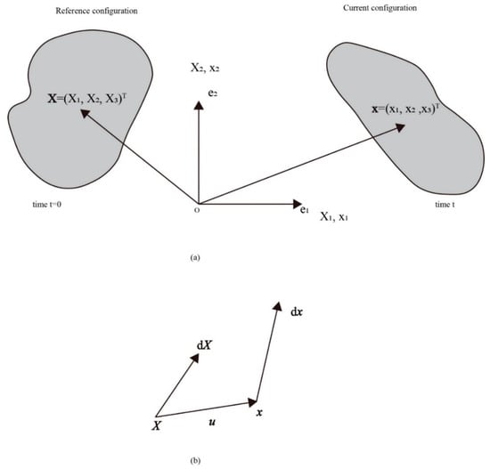
Figure 1.
Reference (undeformed) and current (deformed) configurations (modified from [6,31]). (a) Deformation of infinitesimal elements; (b) Deformation of the line element.
The deformation gradient tensor F describes the transformation of a material point from its undeformed reference configuration into its deformed configuration. It is mathematically defined as the gradient of the displacement field [6,31], as follows:
In component form, as follows:
Using Equations (1) and (2), F is the Jacobi matrix. It can be abbreviated as follows:
where is the displacement vector, is the displacement gradient tensor, and is the identity tensor.
The deformation gradient tensor F in matrix form is as follows:
The Jacobian determinant J of F is as follows:
It describes the volumetric change during deformation [6,31].
Key concepts in large deformation theory include the Green strain tensor and the Cauchy stress tensor, which are suited for nonlinear deformations. Constitutive equations must also be developed to accurately capture material behavior under large deformations. This theory is crucial for predicting the mechanical responses of materials and structures in scenarios involving significant, nonlinear deformations, with a wide applicability in real-world engineering problems.
2.2. Green Strain Tensor and Cauchy Stress Tensor
The squared difference in length between the undeformed element dX and deformed element dx defines the Green strain tensor E, as follows [6,31]:
where dS and ds are the lengths of the undeformed and deformed elements, respectively. The Green strain tensor E, referenced to the undeformed configuration, is given by the following [6,31]:
Expanding this:
In component form, this becomes the following:
The second Piola–Kirchhoff stress tensor is related to the Green strain tensor E by the following:
where λ and μ are the Lamé constants, related to the elastic modulus E and Poisson’s ratio as and . δij are the Kronecker delta tensor representing an identical matrix.
For large elastic deformations, the Cauchy stress tensor σ must be used, and its relationship with the second Piola–Kirchhoff stress tensor P is expressed as follows [6,31]:
The second Piola–Kirchhoff stress P represents the virtual stress in the undeformed configuration and is considered to be a pseudo-stress tensor. The expanded form of the Cauchy stress tensor σ is as follows:
The index notation expression for the Cauchy stress tensor is as follows:
2.3. Parallel Finite Element Implementation of Elastic Large Deformation Theory
Due to the nonlinearity of the Green strain tensor and the Cauchy stress tensor with respect to displacement, implementing elastic large deformation theory via the finite element method is more challenging than for small deformations. To simplify, the Green strain tensor is split into a linear part and a nonlinear part [36,37,38,39,40,41,42].
For convenience in the finite element formulation, the large displacement vector is denoted as , v and the undeformed coordinates as . The linear strain part is expressed as follows:
or in component form as follows:
To express the nonlinear part and derive the virtual work equation for elastic large deformation, we define the following [40,41]:
The Green strain tensor is, thus, written as follows:
The weak form of the finite element equation for large elastic deformations is as follows [40,41]:
The operator F is defined as follows [40,41]:
The final weak solution is as follows [40,41]:
where w is the displacement to be solved for the linear equation after linearization by Newton’s method, u is the known displacement of the last iteration step after linearization, and δu represents the virtual displacement. and denote the body force and surface force on the stress boundary in the study region, respectively, and denotes the linear elastic material matrix. denotes the volume integral of the inner product of the two quantities to the left and right of the semicolon in a finite element cell or the area integral in a boundary cell, and can be used to conveniently characterize the weak form of a finite element equation. The final weak solution Equation (23) can be easily generated automatically in the PFELAC 2.2 software platform as a parallel finite element program in the C language version [40,41].
The PFELAC software platform can automatically generate parallel programs based on elastic large deformation finite element formulations [42,43,44,45]. We developed a parallel finite element program for elastic large deformation analysis based on the principle of virtual work, using the PFELAC 2.2 platform [40,41,42]. The program utilizes a domain decomposition approach for parallelization, with a master process responsible for assembling the global stiffness matrix and load vector, while multiple sub-processes handle the computation of element-level stiffness matrices and load vectors. Parallel computing is implemented using the domain decomposition method, which divides the task into a main process and several sub-processes [42]. Using “test” as the project name, the complete set of parallel elastic large deformation programs is generated, with the architecture illustrated in Figure 2.
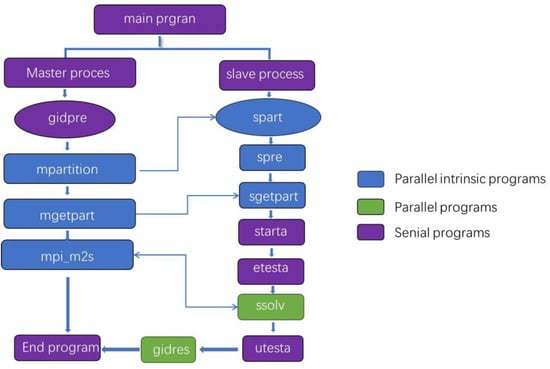
Figure 2.
PFELAC 2.2 parallel program architecture for elastic large deformation analysis [43,44].
The FELAC software platform outputs each partition individually. For example, if the project name is “test” and it is computed in three partitions, the post-processing files with mesh grids and displacement and stress results generated are the following:
- test1.post.msh, test2.post.msh, test3.post.msh…
- test1.post.res, test2.post.res, test3.post.res…
These partitioned results can be merged using GID (12.0.6) software to view the complete post-processing output.
The PFELAC software platform has several advantages over FEPG [43,44], as follows:
- (1)
- It offers a better stability and maintainability with C language compared to Fortran.
- (2)
- The main program flow is simpler, requiring automatic generation only for different problems.
- (3)
- PFELAC includes features for controlling nonlinear problems, providing more flexibility than FEPG’s communication methods.
- (4)
- Point-to-point communication in PFELAC is more efficient than FEPG’s master–slave approach.
- (5)
- PFELAC reduces computation time by eliminating the need to send result data back to the main process.
- (6)
- The results are partition-specific, with no need to consolidate them in the main process.
- (7)
- The parallel computing workflow is streamlined, removing the need for data conversion and additional pre/post-processing steps. After uploading the source code to the server, it simply needs to be compiled and executed.
We employed the bi-conjugate gradient stabilization (BiCGSTAB) method, a variant of the bi-conjugate gradient (BiCG) method, for solving nonsymmetric matrices. The iterative algorithm terminated when the relative residuals were below . For the same situation, the number of CPU cores is 1, 4, 16 and 64 respectively. The simulations were run on Huawei’s TaiShan 200 (2280) server (Huawei Technologies Co., Ltd., Shenzhen, China), equipped with two 48-core Kunpeng 920 processors (Huawei Technologies Co., Ltd., Shenzhen, China), four 32 GB DDR4 RDIMM modules (Huawei Technologies Co., Ltd., Shenzhen, China), and four 1200 GB general-purpose hard drives (Unisplendour Co., Ltd., Beijing, China).
3. Parallel Finite Element Program Verification: Two Ideal Cases of Elastic Large Deformation
In this study, we selected two idealized models of elastic large deformation [34], incorporating rotational, tensile, and shear deformations with known analytical solutions to validate our independently developed parallel finite element program. This program, built on the PFELAC 2.2 platform and written in C language, was optimized for parallel computation, unlike the previous Fortran-based version [34].
3.1. Case 1: Elastic Large Deformation with 45° Stretching and Rotation
The initial configuration is a 1 m × 1 m × 0.01 m square sheet (dashed lines in Figure 3). The sheet undergoes large elastic deformation with a constant thickness. First, it is stretched in both directions, increasing the side length by a factor of . Then, the sheet is rotated 45° counterclockwise, resulting in the final configuration (solid lines in Figure 3). The material properties are a Young’s modulus of and Poisson’s ratio of 0.25.
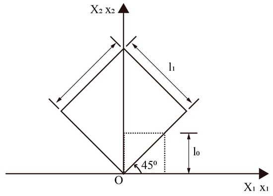
Figure 3.
Schematic of the ideal model for tensile and rotational elasticity in parallel program testing [34]. The side lengths of the square before and after deformation are l0 = 1 m and l1 =, respectively.
The relationship between the post-deformation coordinates and the pre-deformation coordinates for the 45° rotational tensile elastic deformation is given by the following [34]:
The displacement gradient matrix for this model is as follows:
The determinant of , J, is as follows:
The Green strain tensor is as follows:
Using a Young’s modulus E = and Poisson’s ratio ν = 0.25, we find λ = µ = . The Piola–Kirchhoff stress tensor is as follows:
The Cauchy stress tensor is as follows:
The displacement vector at the center of the model is as follows:
We establish a parallel elastic finite element model (Model A) with a residual accuracy of based on Case 1 (Figure 3). Figure 4 presents contour plots of the total displacement and nonzero stress components from Model A’s intermediate section. The color scale’s upper and lower limits represent the maximum and minimum computational values. The displacement results indicate a 45-degree rotation and stretching of the square plate (Figure 4a). The stress components are all homogeneous (Figure 4b–d).
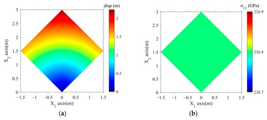
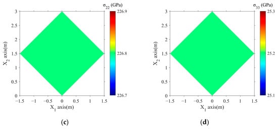
Figure 4.
Total displacement and nonzero stress components from Model 3. (a) Total displacement, (b) normal stress , (c) normal stress , and (d) normal stress .
To examine the influences of node count and parallel partitions on large elastic deformation, we developed four parallel elastic finite element models (Models 1–4) based on Case 1 (Figure 3). Models 1, 2, and 3, each with four parallel partitions, contained 20,000, 2 million, and 8 million nodes, respectively. Model 4, with 24 parallel partitions, also contained 8 million nodes.
We compared the displacement components and the six components of the Cauchy stress tensor at the center point from the simulations of Models 1, 2, 3, and 4 with the analytical solutions (Table 1). Both the displacement and stress fields showed excellent agreement with the analytical results.

Table 1.
Comparison of center point displacements and stresses and parallel calculation time from parallel finite element Models 1–4 with analytical solutions for 45° tensile and rotational elastic large deformation (Case 1). Serial calculations in the larger groupings of the models (Models 2–4) could not be run at this time, so there is no corresponding runtime.
3.2. Case 2: Elastic Large Deformation Under Simple Shear
In Case 2, a 1 m × 1 m × 0.01 m square thin plate (outlined by dashed lines in Figure 5) undergoes elastic large deformation [34]. The lower boundary is fixed while the upper boundary experiences simple shear, resulting in a shear angle of α = 45°, transforming the square into a parallelogram (outlined by solid lines in Figure 5). The elastic material properties are a Young’s modulus of and Poisson’s ratio of 0.25.
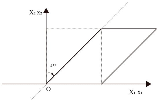
Figure 5.
Schematic of a simple shear ideal model for parallel program testing. (α = 45°, [34]).
The relationship between the post-deformation coordinates and the pre-deformation coordinates for the simple shear elastic large deformation model (with ) is given by the following [34]:
The displacement gradient matrix F for this model is as follows:
with a determinant of J = 1. The Green strain tensor E is as follows:
With a Young’s modulus E = and Poisson’s ratio ν = 0.25, we find λ = µ = .
The stress tensor P is computed as follows:
The Cauchy stress tensor is as follows:
For validation, the displacement vector at the model’s center is as follows:
We establish a parallel elastic finite element model (Model B) with a residual accuracy of based on Case 2 (Figure 5). Figure 6 shows contour plots of the total displacement and nonzero stress components for the intermediate sections from the simulations of Model B. The color scale limits represent the maximum and minimum values of each result. The displacement field confirms a 45-degree simple shear deformation (Figure 6a). The four nonzero stress components () are uniform across the model (Figure 6b–e).
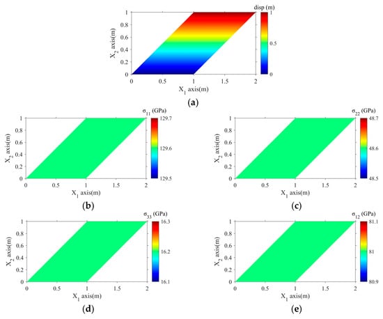
Figure 6.
Results from Model 7: (a) total displacement magnitude, (b) normal stress , (c) normal stress , (d) normal stress , and (e) shear stress .
To analyze the effects of node count and partitioning on large deformations, we developed four parallel finite element models (Models 5–8) for Case 2 (Figure 5). Models 5, 6, and 7 used four parallel partitions with node counts of 2 × 100 × 100, 2 × 1000 × 1000, and 2 × 2000 × 2000, respectively. Model 8 used 24 parallel partitions with 2 × 2000 × 2000 nodes.
We compared the displacement components at the center point and the six components of the Cauchy stress tensor from Models 5, 6, 7, and 8 with the corresponding analytical solutions (Table 2). The displacement and stress fields of the parallel finite element models showed excellent agreement with the analytical results.
Table 2.
Comparison of center point displacements and stresses and parallel calculation time with analytical solutions for parallel Models 5, 6, 7, and 8 under simple shear large deformation.
For Models 1, 2, 3, and 4 of Case 1, the parallel running times are 7.67, 773, 3160, and 739 s, respectively, and for Models 5, 6, 7, and 8 of Case 2, the parallel running times are 7.66, 776, 3210, and 755 s, respectively.
In parallel computing, Speedup and Efficiency are two important performance metrics [46,47]. Speedup is defined as follows [47]:
where is Speedup, is the running time of the serial algorithm while executing the task, and is the running time of the serial algorithm while executing the same task using p processors.
Efficiency is defined as follows [47]:
where is Efficiency and the rest of the variables are the same as in the above equation.
Table 3 gives the computation time, Speedup (), and Efficiency () for different numbers of cores (1, 4, 16, and 64) for Models 1–3 and Models 5–7. It is found that the greater the number of cores, the greater the parallel acceleration ratio, which is in the range of 3.70–3.80 for 4 cores, 11.36–12.24 for 16 cores, and 24.70–34.78 for 64 cores. This indicates that the computation time of the same task can be greatly reduced by using multi-core parallel computation, compared with single-core serial computation. In addition, the 4-core parallel efficiency is the highest, at up to 0.93–0.94, the 64-core parallel efficiency is the lowest, at 0.39–0.43, and the 16-core parallel efficiency is more than 0.5, in the range of 0.71–0.77, which is a very good parallel efficiency in general.
Table 3.
Comparison of calculation time, Speedup, and Efficiency for Serial (1 core) and Parallel (4, 16, and 64 cores) for different models (the values in the table are calculation time (in seconds), Speedup, and Efficiency, respectively).
4. Real-World Application
Fold deformation over geological time typically involves significant crustal shortening, leading to large rather than small deformations. We modeled a vertical profile with a thickness of 1 km, spanning 6 km in length and 2.5 km in depth, featuring two layers of folds at the top and bottom (Figure 7). The two yellow bands represent crustal folds at different depths, with a Young’s modulus of and a Poisson’s ratio of 0.25, while the green area represents the surrounding stratigraphic medium with a Young’s modulus of and the same Poisson’s ratio. The right and bottom boundaries have zero normal displacement constraints and allow for free sliding tangentially, while the left boundary applies horizontal compressive displacement, vertical free sliding, and an unconstrained ground surface.
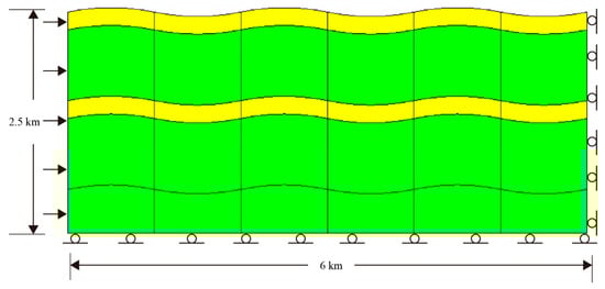
Figure 7.
Geometric model illustrating fold deformation over geological time. The model has a length of 6 km and a depth of 2.5 km, featuring two layers of folds above and below. The yellow bands represent crustal folds at varying depths, while the green area denotes the surrounding stratigraphic medium. The left boundary experiences uniform horizontal compression with free sliding in tangent direction, as indicated by a transverse arrow. The upper boundary is unconstrained, while the other boundaries prevent normal displacement and allow tangential sliding, represented by planar rollers.
To compare the effects of large and small elastic deformations on fold belt evolution, we built four models with identical geometry, material properties, and boundary conditions, differing only in their left boundary displacement. In Models C and D, the left boundary underwent 1 km of horizontal compression with a tectonic shortening rate of 1/6, representing large deformation. Displacement and stress fields were calculated using large and small deformation theories, respectively. In Models E and F, the left boundary experienced 6 m of compression with a shortening rate of 1/1000, characteristic of small deformation, with both large and small deformation theories applied for comparison.
Model C for elastic small deformation and Model D for elastic large deformation were used to compare the differences in the displacement and stress fields simulated by the elastic large deformation model and the elastic small deformation model (the left boundary underwent 1 km of horizontal compression with the same large tectonic shortening rate of 1/6). A comparison of the displacement and stress fields highlights the characteristics and advantages of the large deformation model (Figure 8 and Figure 9). The displacement components u and v show minor differences between Models C and D, while the vertical component w exhibits significant variation (Figure 8). The differences in the nonzero stress components () are substantial, whereas remain near zero (Figure 9). This comparison demonstrates that, for large elastic deformations, such as a horizontal shortening of 1/6, large deformation theory is essential for accurate results. Using small deformation theory would lead to significant errors in both displacement and stress fields.
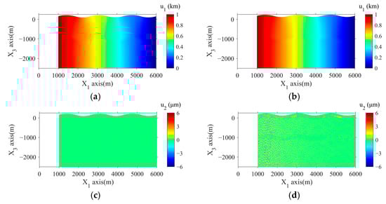
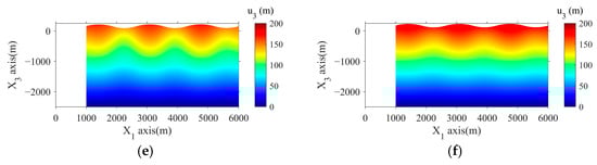
Figure 8.
Comparison of displacement fields between the elastic large deformation model (Model C, elastic large deformation theory) and the elastic small deformation model (Model D, elastic small deformation theory) with the same large tectonic shortening rate of 1/6. Left column: displacement u, v, and w components by Model C (panels (a,c,e)). Right column: u, v, and w components by Model D (panels (b,d,f)).
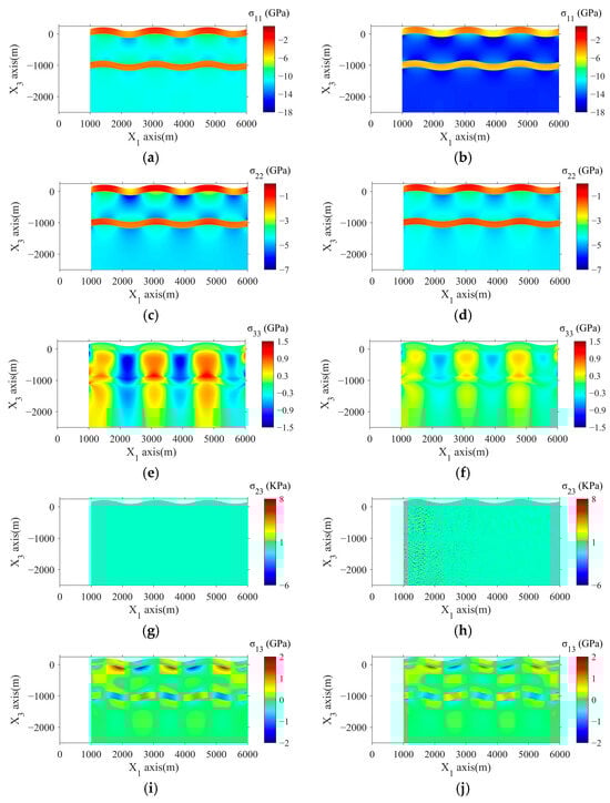
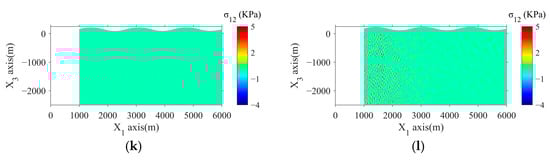
Figure 9.
Comparison of stress fields between the elastic large deformation model (Model C) and the elastic small deformation model (Model D). Left column: stress components by Model C (panels (a,c,e,g,i,k)), Right column: stress components by Model D (panels (b,d,f,h,j,l)).
5. Discussion and Conclusions
When the strain is minimal, the results from large deformation theory closely align with those from small deformation theory. However, with substantial strain, discrepancies between the two theories become pronounced, particularly in stress results. This underscores the critical role of large deformation theory in studying crustal deformation over geological timescales (~Ma). Relying solely on small deformation theory for such studies could lead to significant inaccuracies in stress predictions (Figure 10). Note that the color bar units of the corresponding pictures on the left and right sides of Figure 10 are sometimes different, e.g., the unit of Figure 10e is m while the unit of Figure 10f is mm, and the unit of Figure 10g is GPa while the unit of Figure 10h is MPa.
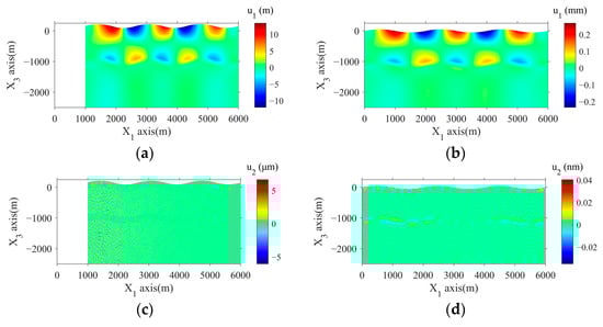
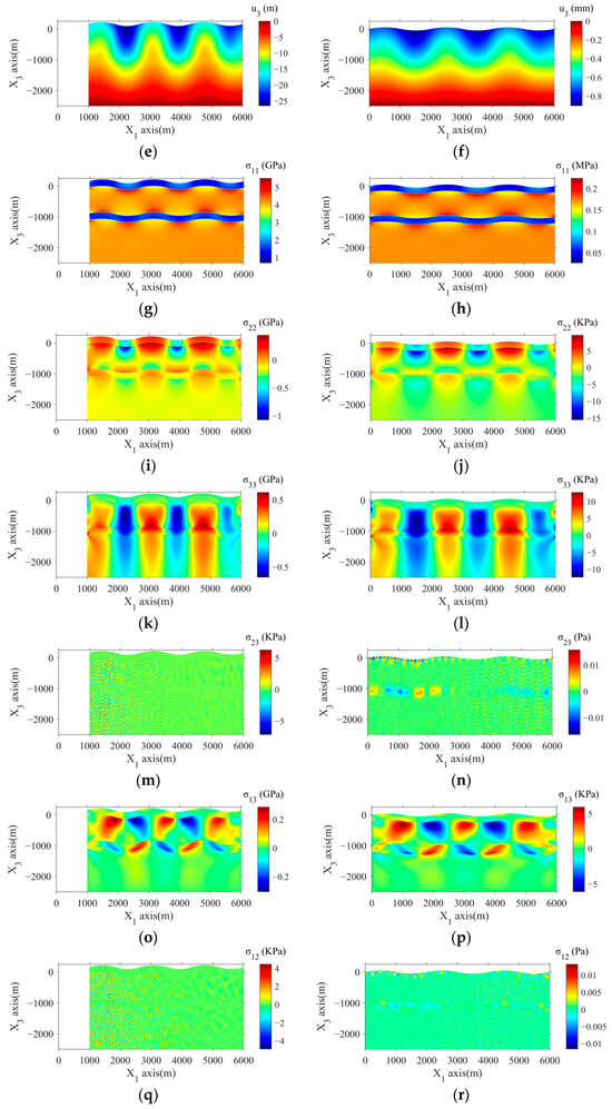
Figure 10.
Differences in results between large and small deformation models for compressions of 1000 m (1/6) and 6 m (1/1000). Left column: displacement components u, v, w, and stress components by Models C and D (panels (a,c,e,g,i,k,m,o,q)), Right column: displacement components u, v, w, and stress components by Models E and F (panels (b,d,f,h,j,l,n,p,r)).
Figure 10 compares the displacement and stress components from numerical simulations of large and small deformations. The left column shows the results for Models C and D with a shortening rate of 1/6, while the right column shows the results for Models E and F with a shortening rate of 1/1000. The differences in the displacement (u and w) and stress components () are significantly larger in Models C and D than in Models E and F. These results indicate that when the structural shortening reaches the large deformation threshold (e.g., 1/6), large deformation theory must be used for accurate calculations. In contrast, for smaller deformations (e.g., 1/1000), the differences are minimal, allowing for the use of small deformation theory to reduce computational cost.
Elastic large deformation is prevalent in crustal and geo-engineering contexts, garnering increasing attention [35]. Unlike linear elastic small deformation, elastic large deformation is characterized by nonlinear geometric equations [6,31]. Key to this theory is the Green strain tensor, coupled with the Cauchy stress tensor, both of which exhibit nonlinear relationships with displacement [6,31]. The finite element formulation for large deformations is inherently nonlinear and requires iterative solutions [36,40,41,42]. We compared the computation times of 1, 4, 16, and 64 cores from different models and quantitatively evaluated the Speedup and parallel Efficiency of our parallel finite element program for elastic large deformation.
The sources of numerical error in the finite element calculations primarily include the finite nature of the mesh (up to 8 million cells), interpolation errors arising from the choice of shape functions, and the truncation errors associated with the nonlinear iterative algorithm. The numerical error in the displacement field is generally smaller, whereas the error in the stress field is larger due to the least squares method used for stress computation, which does not yield absolute accuracy in the simulated stress values at the nodes. The application case of crustal tectonic shortening is chosen because it is a common geological phenomenon that effectively illustrates the differences between large and small deformation theories. This case serves as a valuable research tool for the numerical simulation of tectonic deformation in more complex scenarios, such as globally distributed folded thrust belts.
Finally, we draw the following three conclusions:
- In this study, we developed a parallel finite element program for elastic large deformation using the PFELAC software platform. We validated this program by comparing its results with analytical solutions from the following two conceptual models: a 45-degree rotated tensile large deformation model and a simple shear large deformation model.
- The comparison with results from the small deformation theory, exemplified by a fold-large deformation case, demonstrated the necessity of accounting for geometric nonlinearity in real crustal deformation studies. The Green strain tensor’s nonlinear relation to displacements highlighted its significance when paired with the Cauchy stress tensor.
- The higher the number of cores, the greater the parallel acceleration ratio, but the lower the parallel efficiency. For 16 cores, the acceleration ratio was 11.36–12.24 and the parallel efficiency was 0.71–0.77, and for 64 cores, the acceleration ratio was 24.70–34.78 and the parallel efficiency was 0.39–0.43. The parallel acceleration ratios and parallel efficiencies of our parallel resilient large model program were excellent.
Author Contributions
Conceptualization, C.H.; Methodology, C.H. and H.Z.; Software, Y.C., C.H. and H.Z.; Validation, Y.C. and C.H.; Writing—original draft, Y.C. and C.H.; Writing—review & editing, Y.C. and H.Z.; Visualization, Y.C.; Project administration, C.H. and H.Z.; Funding acquisition, C.H. and H.Z. All authors have read and agreed to the published version of the manuscript.
Funding
This research was funded by the National Key Research and Development Program of China (Grant Nos. 2023YFF0804300, 2023YFF0804301), National Natural Science Foundation of China (Grant No. 42374116) and Fundamental Research Funds for the Central Universities (E2ET0413X2).
Data Availability Statement
The original contributions presented in the study are included in the article, further inquiries can be directed to the corresponding authors.
Acknowledgments
Parallel finite element calculations were run on the GeoModeling Cluster at UCAS and Beijing Super Computing Center. We thank Yuanze Zhou and Yongfa Zhou for some useful discussions on numerical simulation.
Conflicts of Interest
The authors declare no conflict of interest.
References
- Wang, D.; Jiang, Y.; Sun, X.; Luan, H.; Zhang, H. Nonlinear Large Deformation Mechanism and Stability Control of Deep Soft Rock Roadway: A Case Study in China. Sustainability 2019, 11, 6243. [Google Scholar] [CrossRef]
- Liu, W.; Chen, J.; Chen, L.; Luo, Y.; Shi, Z.; Wu, Y. Nonlinear Deformation Behaviors and a New Approach for the Classification and Prediction of Large Deformation in Tunnel Construction Stage: A Case Study. Eur. J. Environ. Civ. Eng. 2020, 26, 1–29. [Google Scholar] [CrossRef]
- Sui, Q.; He, M.; He, P.; Xia, M.; Tao, Z. State of the Art Review of the Large Deformation Rock Bolts. Undergr. Space 2022, 7, 465–482. [Google Scholar] [CrossRef]
- Ma, D.; Tan, Z.; Bian, L.; Zhang, B.; Zhao, J. Research on Deformation and Loose Zone Characteristics of Large Cross Section Tunnel in High Geo-Stress Soft Rock. Appl. Sci. 2023, 13, 9009. [Google Scholar] [CrossRef]
- Tang, L.; Zhang, Z. Prediction and Classification of Large Deformations in Deep Tunnels Based on Stress Inversion Method. Geotech. Geol. Eng. 2023, 41, 2343–2358. [Google Scholar]
- Malvern, L.E. Introduction to the Mechanics of a Continuous Medium; Prentice-Hall, Inc.: Englewood Cliffs, NJ, USA, 1969; p. 713. [Google Scholar]
- Jeremic, B.; Runesson, K.; Sture, S. Finite Deformation Analysis of Geomaterials. Int. J. Numer. Anal. Meth. Geomech. 2001, 25, 809–840. [Google Scholar] [CrossRef]
- Hashiguchi, K.; Yamakawa, Y. Introduction to Finite Strain Theory for Continuum Elasto-Plasticity; John Wiley & Sons, Ltd.: Hoboken, NJ, USA, 2013. [Google Scholar] [CrossRef]
- Shabana, A.A. Computational Continuum Mechanics, 3rd ed.; Wiley: Hoboken, NJ, USA, 2018; pp. 1–350. [Google Scholar]
- Soga, K.; Alonso, E.; Kumar, K.; Bandara, S. Trends in Large-deformation Analysis of Landslide Mass Movements with Particular Emphasis on the Material Point Method. Géotechnique 2016, 3, 248–273. [Google Scholar] [CrossRef]
- Zhang, X.; Sheng, D.; Sloan, S.W.; Bleyer, J. Lagrangian Modelling of Large Deformation Induced by Progressive Failure of Sensitive Clays with Elastoviscoplasticity. Int. J. Numer. Meth. Eng. 2017, 112, 963–989. [Google Scholar] [CrossRef]
- Liu, B.; Wang, W.; Liu, Z.; Ouyang, N.; Mao, K.; Zhou, F. Study on Large Deformation of Soil–rock Mixed Slope Based on GPU Accelerated Material Point Method. Sci. Rep. 2024, 14, 6983. [Google Scholar] [CrossRef]
- Milliner, C.; Donnellan, A.; Aati, S.; Avouac, J.P.; Zinke, R.; Dolan, J.F.; Wang, K.; Burgmann, R. Bookshelf Kinematics and the Effect of Dilatation on Fault Zone Inelastic Deformation: Examples from Optical Image Correlation Measurements of the 2019 Ridgecrest Earthquake Sequence. J. Geophys. Res. Solid Earth 2021, 126, e2020JB020551. [Google Scholar] [CrossRef]
- He, M.C.; Xie, H.P.; Peng, S.P.; Jiang, Y.D. Study of Rock Mechanics in Deep Mining Engineering. Chin. J. Rock Mech. Eng. 2005, 16, 2803–2813. (In Chinese) [Google Scholar] [CrossRef]
- Mcivor, M.; Anderson, W.J.; Buak-Zochowski, M. An Experimental Study of the Large Deformation of Plastic Hinges. Int. J. Solids Struct. 1977, 13, 53–61. [Google Scholar] [CrossRef][Green Version]
- Lubliner, J. Normality Rules in Large-deformation Plasticity. Mech. Mater. 1986, 5, 29–34. [Google Scholar] [CrossRef]
- Sakai, Y.; Yamasita, A. Elastic-plastic Large Deformation Analysis Using SPH. In Computational Methods; Liu, G.R., Tan, V.B.C., Han, X., Eds.; Springer: Berlin/Heidelberg, Germany, 1986; pp. 1515–1519. [Google Scholar]
- Guo, Z.; Watanabe, O. Study on Accuracy of Finite-Element Solutions in Elastoplastic Large Deformation. JSME Int. J. Ser. A 1996, 39, 99–107. [Google Scholar]
- Levin, V.A.; Taras’ev, G.S. One Variant of the Model of a Viscoelastic Body at Large Deformations. Sov. Appl. Mech. 1983, 19, 615–618. [Google Scholar] [CrossRef]
- Chandra, A.; Mukherjee, S. Boundary Element Formulations for Large Strain-large Deformation Problems of Viscoplasticity. Int. J. Solids Struct. 1984, 20, 41–53. [Google Scholar] [CrossRef]
- Pai, P.F.; Palazotto, A.N. Large-deformation Analysis of Flexible Beams. Int. J. Solids Struct. 1996, 33, 1335–1353. [Google Scholar] [CrossRef]
- Takanoa, N.; Ohnishia, Y.; Zakoa, M.; Nishiyabu, K. The Formulation of Homogenization Method Applied to Large Deformation Problem for Composite Materials. Int. J. Solids Struct. 2000, 37, 6517–6535. [Google Scholar] [CrossRef]
- Akhundov, V.M. A 4D Composite Reinforced along Cube Diagonals with a Small Content of Yarns under Large Tensile Deformations. Mech. Compos. Mater. 2002, 38, 197–210. [Google Scholar]
- Akhundov, V.M. A 4D Composite Reinforced along Cube Diagonals with a Small Content of Yarns under Large Shear Deformations. Mech. Compos. Mater. 2002, 38, 215–222. [Google Scholar] [CrossRef]
- Gu, Y.T. An Adaptive Local Meshfree Updated Lagrangian Approach for Large Deformation Analysis of Metal Forming. Adv. Mater. Res. 2010, 97–101, 2664–2667. [Google Scholar] [CrossRef]
- Chekhov, V.V. Matrix FEM Equation Describing the Large-strain Deformation of an Incompressible Material. Int. Appl. Mech. 2011, 46, 1147–1153. [Google Scholar] [CrossRef]
- Wu, Y.Z.; Zhu, Y.P.; Dui, G.S. Influence of Small-strain and Large-strain Methods on Mechanical Behaviors in Shape Memory Alloys. Adv. Mater. Res. 2011, 328–330, 1556–1559. [Google Scholar] [CrossRef]
- Kumar, R.; Singh, I.V.; Mishra, B.K.; Singh, A. Numerical Simulation of Large Deformation Problems by Element Free Galerkin Method. Key Eng. Mater. 2013, 535–536, 85–88. [Google Scholar] [CrossRef]
- Davydov, R.L.; Sultanov, L.U. Numerical Algorithm for Investigating Large Elasto-plastic Deformations. J. Eng. Phys. Thermophys. 2015, 88, 1280–1288. [Google Scholar] [CrossRef]
- Ma, Y.; Zhou, Y. Hybrid Natural Element Method for Large Deformation Elastoplasticity Problems. Chin. Phys. B 2015, 24, 030204. [Google Scholar] [CrossRef]
- Iai, S. Developments in Earthquake Geotechnics. Geotech. Geol. Earthq. Eng. 2018, 43, 367–409. [Google Scholar] [CrossRef]
- He, M. High Slope Engineering of Open Pit Mine; China Coal Industry Publishing House: Beijing, China, 1991. (In Chinese) [Google Scholar]
- He, M. General Theory of Soft Rock Tunnel Engineering; China University of Mining and Technology Press: Xuzhou, China, 1993. (In Chinese) [Google Scholar]
- He, M.; Chen, X.; Liang, G.; Qian, H.; Zhou, Y.; Zhuang, X. Software System for Large Deformation Mechanical Analysis of Soft Rock Engineering at Great Depth. Chin. J. Rock Mech. Eng. 2007, 26, 934–943. (In Chinese) [Google Scholar]
- He, M.; Sui, Q.; Tao, Z. Excavation Compensation Theory and Supplementary Technology System for Large Deformation Disasters. Deep Undergr. Sci. Eng. 2023, 2, 105–128. [Google Scholar] [CrossRef]
- Yin, Y. Introduction to Nonlinear Finite Elements in Solid Mechanics; Peking University Press: Beijing, China, 2007. [Google Scholar]
- Hu, C. A New Method to Study Earthquake Triggering and Continuous Evolution of Stress Field. Ph.D. Thesis, Peking University, Beijing, China, 2009. [Google Scholar]
- Hu, C.; Zhou, Y.; Cai, Y.; Wang, C. Study of Earthquake Triggering in a Heterogeneous Crust Using a New Finite Element Model. Seismol. Res. Lett. 2009, 80, 799–807. [Google Scholar] [CrossRef]
- Hu, C.; Cai, Y.; Wang, Z. Effects of Large Historical Earthquakes, Viscous Relaxation, and Tectonic Loading on the 2008 Wenchuan Earthquake. J. Geophys. Res. Solid Earth 2012, 117, B06410. [Google Scholar] [CrossRef]
- Liang, G.P.; Zhou, Y.F. Finite Element Language and Its Application I; Science Press: Beijing, China, 2015. [Google Scholar]
- Liang, G.P.; Zhou, Y.F. Finite Element Language and its Application II; Science Press: Beijing, China, 2015. [Google Scholar]
- Shi, M.; Meng, S.; Hu, C.; Shi, Y. Crustal Heterogeneity Effects on Coseismic Deformation: Numerical Simulation of the 2008 MW 7.9 Wenchuan Earthquake. Front. Earth Sci. 2023, 11, 1245677. [Google Scholar] [CrossRef]
- Xu, M.; Li, H.; Song, Z.; Xu, Q.; Zhang, X.; Fu, P. An Electric-thermal-solid Physical Fields Coupling Calculation based on FELAC Platform, 2022. In Proceedings of the IEEE 5th International Conference on Electronics Technology, Chengdu, China, 13–16 May 2022; pp. 532–536. [Google Scholar] [CrossRef]
- Element Computing Technology Co., Ltd. Fundamentals and Applications of Finite Element Analysis of FELAC; Element Computing Technology Co., Ltd.: Tianjin, China, 2018; pp. 48–59. (In Chinese) [Google Scholar]
- Element Computing Technology Co., Ltd. Parallel Architecture of FELAC; Element Computing Technology Co., Ltd.: Tianjin, China, 2018; pp. 8–14. (In Chinese) [Google Scholar]
- Amdahl, G.M. Validity of the Single Processor Approach to Achieving Large Scale Computing Capabilities. AFIPS Conf. Proc. 1967, 30, 483–485. [Google Scholar]
- Grama, A.; Gupta, A.; Karypi, G.; Kumar, V. Introduction to Parallel Computing, 2nd ed.; Addison Wesley: Boston, MA, USA, 2003; pp. 1–664. [Google Scholar]


Disclaimer/Publisher’s Note: The statements, opinions and data contained in all publications are solely those of the individual author(s) and contributor(s) and not of MDPI and/or the editor(s). MDPI and/or the editor(s) disclaim responsibility for any injury to people or property resulting from any ideas, methods, instructions or products referred to in the content. |
© 2025 by the authors. Licensee MDPI, Basel, Switzerland. This article is an open access article distributed under the terms and conditions of the Creative Commons Attribution (CC BY) license (https://creativecommons.org/licenses/by/4.0/).