Abstract
In the field of modern drive technology, conventional form-fit shaft-hub connections, such as the standardized keyway connection, are reaching their mechanical limits due to the space-saving design. The trochoidal profiles are elegant modern shaft-hub connections with a compact design for high-power transmission. This article deals with an analytical approach to determining the stress state in trochoidal profiles under shear bending. The solution completes the existing analytical attempts at the load cases of pure bending and torsion. Similar to the torsional loading case, a conformal mapping must be found that can completely transform the unit circle to the non-circle profile area. The conformal mapping function is deduced from the contour equation of the profile. To check the analytical results, in addition, numerical investigations were carried out. The results of the complementary numerical studies show very good agreement with the analytical solutions. The equations derived for the maximum stresses enable a reliable and cost-effective design of the profile shafts subjected to shear force loading.
1. Introduction
The non-circular profiles are an elegant alternative to the conventional shaft-hub connections. These profiles have significant mechanical advantages compared to other form-fit connections such as splined shafts [1]. In recent years, trochoidal profiles have been used due to their higher load-bearing capacity and a clean mathematical description with continuous functions [2,3]. In addition to standard CNC manufacturing processes, simple epitrochoids can be manufactured very economically using the double-spindle turning process [4]. Figure 1 shows some examples produced by [5] using this process.
Figure 1.
Epitrochoidal inner and outer contours for shaft-hub connections produced using the twin-spindle process. Source: Iprotec: Guido Kochsiek [5].
The so-called hypotrochoids, which are related to epitrochoids, also have industrial applications and are standardized according to DIN 3689-1 [6].
The dynamically loaded contact elements often fail inside the connection due to fretting fatigue [7]. In many cases of failure of the non-circular shaft-hub connections, however, failure occurs in the shaft beyond the connection depending on the load magnitude. This issue is discussed for hybrid trochoids in [8].
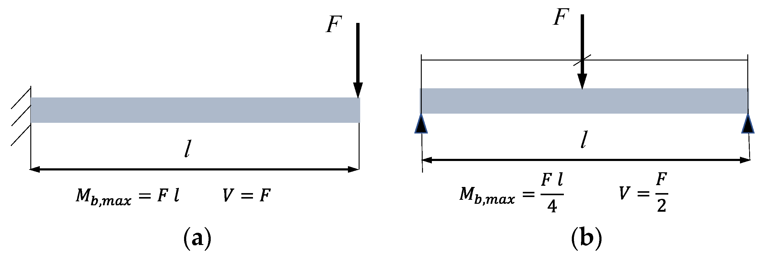
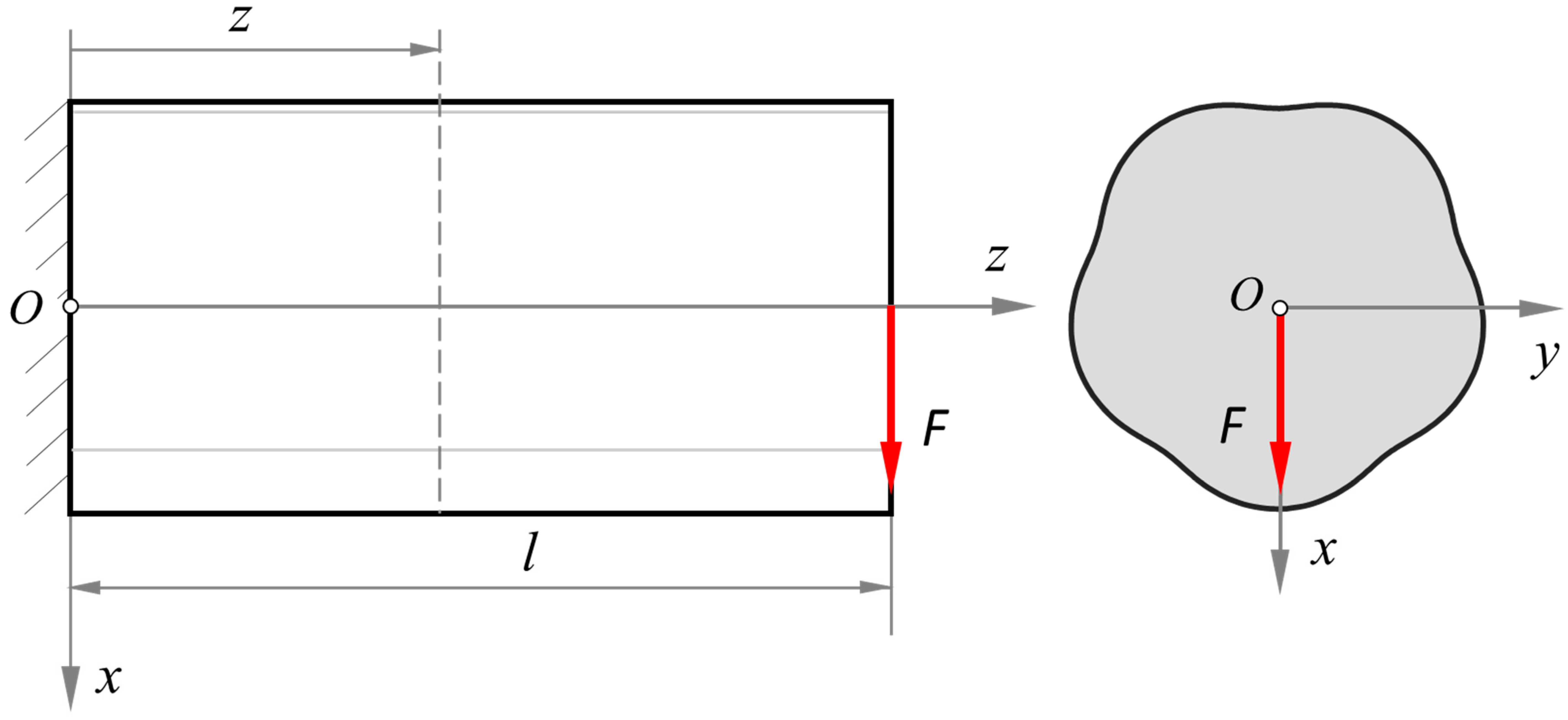
General Considerations of the Lateral Shear Loading
For the design of circular cross-sections, often only the torsional and bending loads are considered and the effects of shear stresses are neglected (see [9]). In non-circular profile shafts, however, the shear stress also has an important influence on the stress state in the shaft. This is particularly the case with short shafts so that the smaller the length ratio , the greater the ratio of the shear stress . For a given length ratio, the relation of shear to bending stress can be determined as a function of the cross-section geometry. For example, the author in [10] determines the ratio / = for a cantilever beam with a square cross-section as shown in Figure 2a. Here, is the side size of the cross-section. This ratio means /, if the length ratio . A similar way can be used to determine the ratio / = for a symmetrically loaded beam with a round cross-section and simple supported as shown in Figure 2b. Here, it means /, if the length ratio . Therefore, for the small design-related length ratios, the transverse shear stresses play a non-negligible role in the strength of the component.
Figure 2.
Effect of support conditions on internal loadings in cantilever beam (a) and in simply supported beam (b).
In many industrial applications in drive technology, the case on the right of Figure 2 is used, where the length ratios can also be in the range of 2.0 to 3.0. In such applications, the magnitude and effects of the transverse shear stresses should be checked.
The classical approach for calculating the lateral shear stress is based on Zhuravsky’s shear model, which was first published around 1855 [11]. Figure 3 shows an example of Zhuravsky’s model for a trochoidal cross-section with three sides, where the distribution of shear stress is assumed to be uniform on the lines parallel to the y-axis.
Figure 3.
Zhuravsky’s model for the example of an epitrochoid with three sides.
The shear stress is determined as a function of the distance x to the neutral axis (y-axis) as follows:
Here, is the first moment of area of the partial surface below the position line and denotes the width of the cross-section at the distance .
The assumption of a uniform distribution of shear stress leads to errors in the solution of the shear stress. The model violates the boundary condition of the free lateral surface as Figure 4a shows (see also [12]), so that a deviation of up to 10% can occur, depending on the Poisson’s ratio for circular cross-sections. Figure 4b shows the real distribution of the shear stress.
Figure 4.
Distribution of shear stress according to the classical parallel distribution approach (a); real shear distribution (b).
In [13], the author introduces a shape coefficient and improves Zhuravsky’s shear model. The effects of Poisson’s ratio are also considered. However, the shape coefficient is dependent on the cross-section geometry and cannot be easily obtained for epitrochoidal cross-sections. Therefore, other more complete and more accurate analytical approaches were applied in this work to determine the shear stresses.
2. Geometrical Description
The non-circular contours used in technical applications are often developed based on general cycloids or trochoids. These curves are also referred to and classified in the technical literature as trochoids [14] and wheel lines [15]. Cycloids can be generated by rolling a circle on a path curve (usually also a circle). Depending on the rolling side, epicycloids, hypocycloids, and hybrid cycloids are produced. If the resulting curve is used as the base curve for a new trochoid, the secondary curve is referred to as a higher-level trochoid. This, in turn, can be used as a new base for further trochoids, whereby the level of the trochoid is increased accordingly.
The general representation and classification of higher-step trochoids is described in detail in [16].
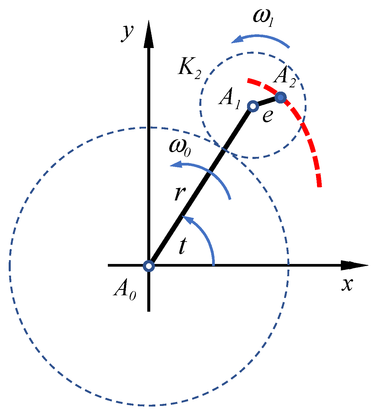
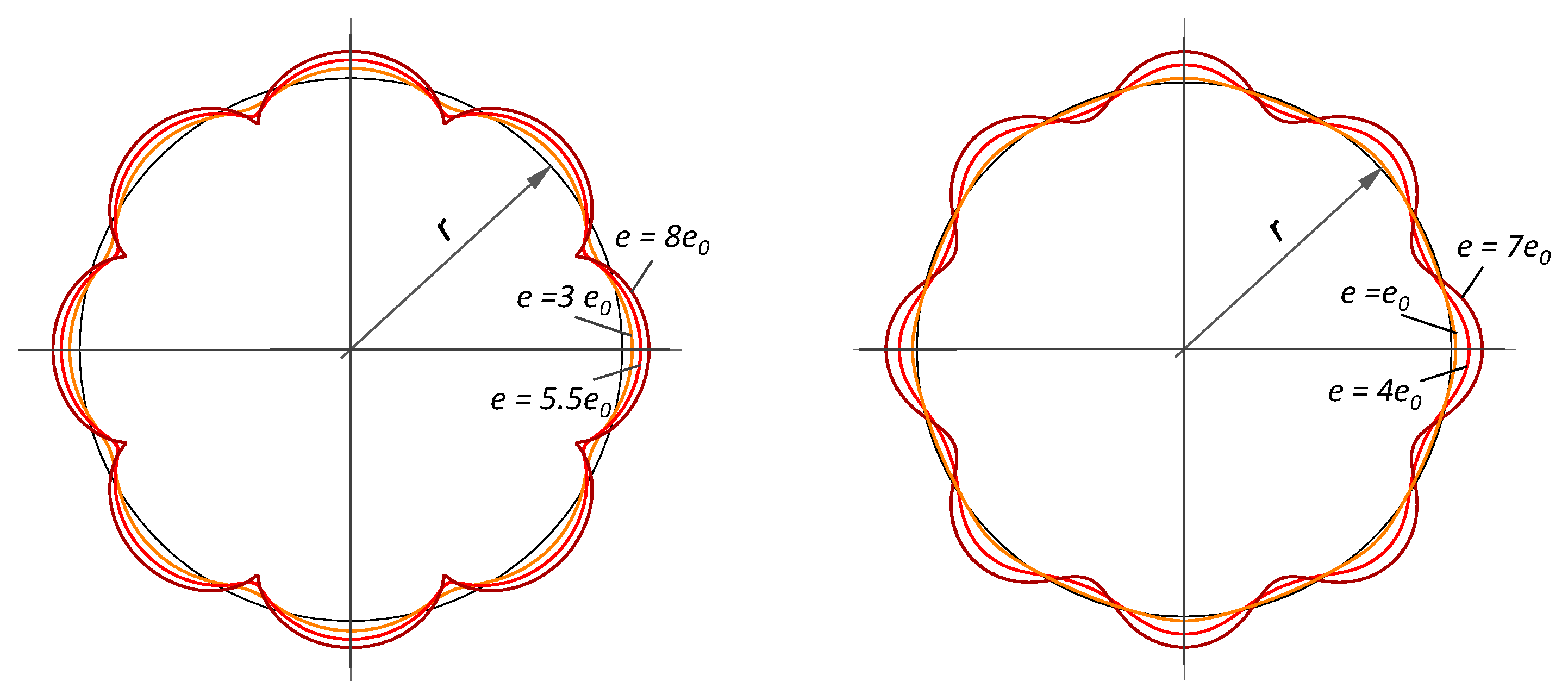
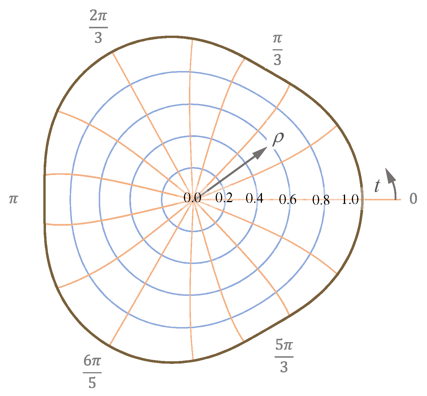
2.1. Simple Epicycloids
Figure 5 shows the generation of a simple epicycloid or a second-stage wheel line. Here, a circle rolls from the outside on a base circle, and point generates a simple epitrochoid with the eccentricity .
Figure 5.
Generation of simple epicycloids.
The geometry of the movement of the generating point can be described as follows:
Here, denotes the nominal radius, the eccentricity, and the periodicity (number of sides) of the cycloids. Equation (1) can be represented as follows by using the complex function:
where and with . If the generation point lies on the circumference of the rolling circle , the path describes a limiting case where the curve begins to cut itself. The eccentricity limit at the intersection of the profile contour is
For an epitrochoid with a flat point (on the flank), the following applies according to [17]:
The epitrochoid with a flat point with was used for the first time in industry as a non-circular polygonal shaft-hub connection. These profiles became known as K-profiles [18] and were the basis of the later standardized P3G profiles [19].
Equation (2) can “conformally” map a unit circle to the profile cross-section. This property plays an important role in determining the stress state in a profile shaft [18].
Figure 6 shows simple epitrochoids with different numbers of flanks based on parametric Equation (1).
Figure 6.
Epitrochoids with different numbers of sides and eccentricities according to Equation (1).
If the rolling circle is on the inside of the base circle, the so-called hypotrochoid results.
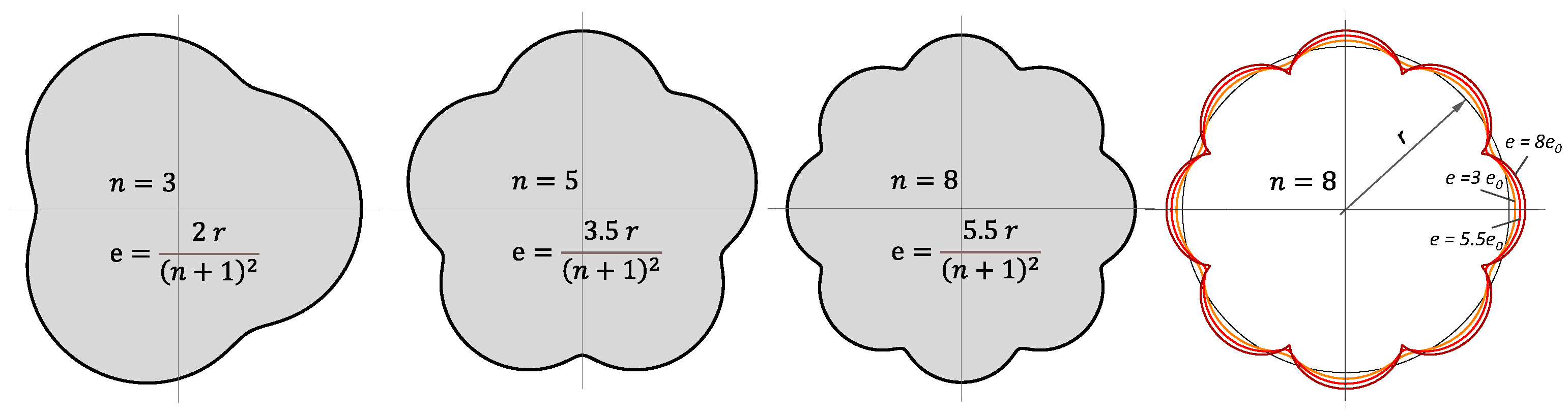
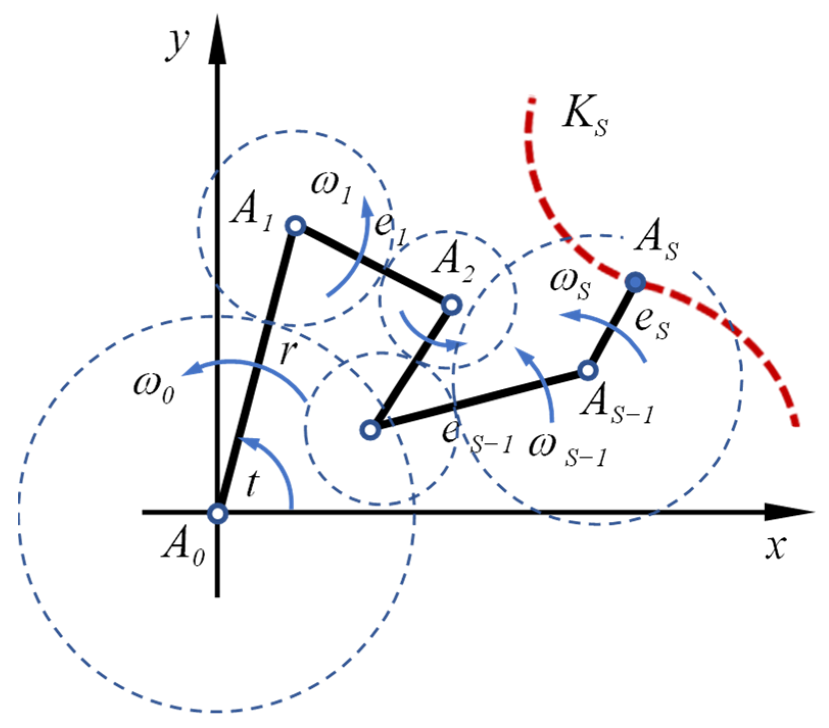
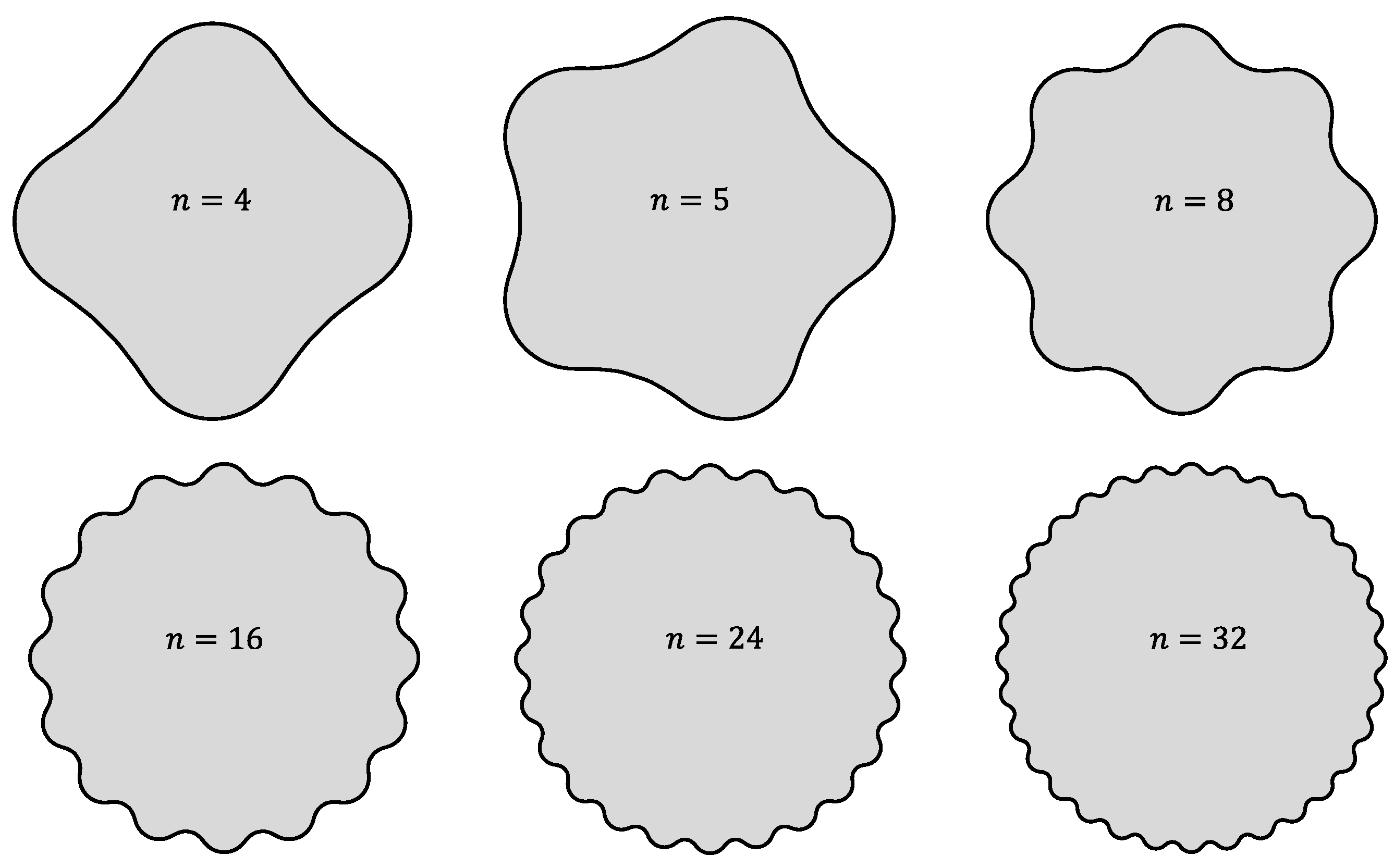
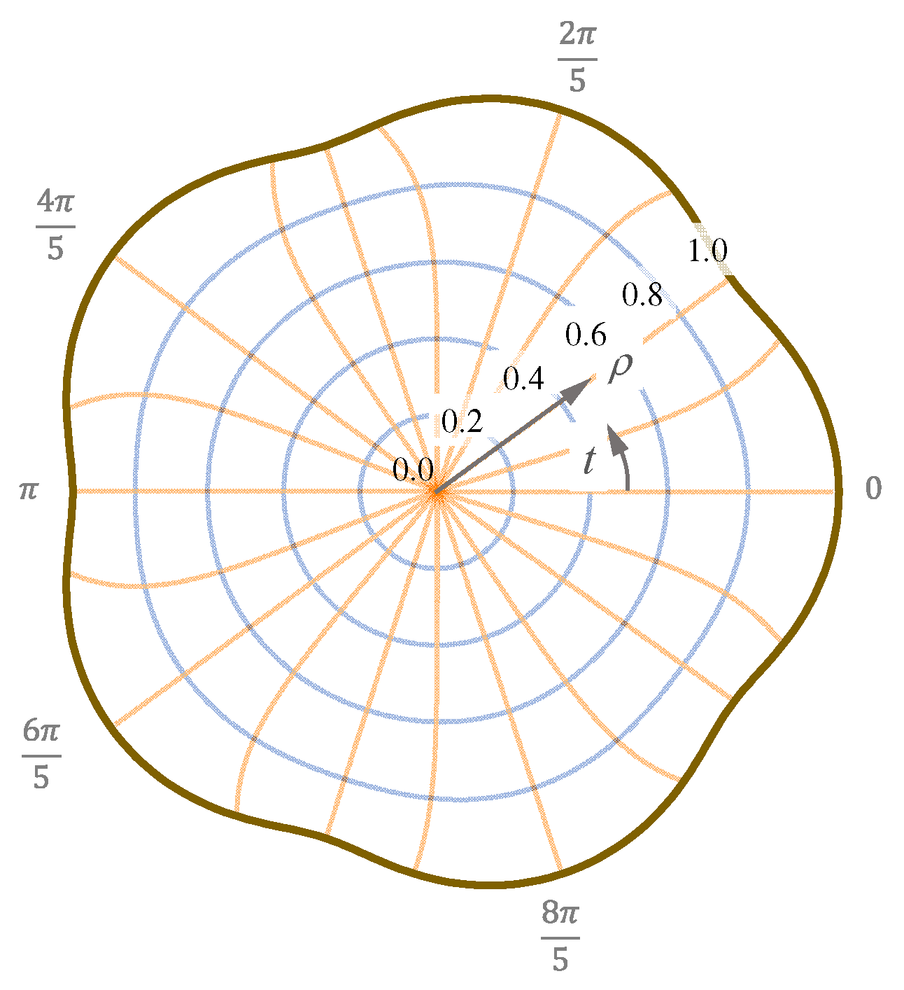
2.2. Higher Epitrochoids
The higher rolling curves were systematically treated for the first time by Wunderlich in [15] with the aid of complex functions. This allows the two-parameter equations to be combined into one complex equation and reduces the mathematical effort. This procedure was also used in [14] for the representation of plane curves. According to Figure 7, the higher epitrochoid is defined by the planetary motion of several levers with the corresponding angular velocities . The position of the creation point is determined by the sum of the vectors , , … and can be determined as follows.
Figure 7.
Generation of the higher epitrochoids.
The following conditions apply to the higher epitrochoids [20]:
Angular velocities, , all act in the same direction and in the positive direction.
where is arbitrary and an integer.
The higher trochoids are described in detail in [20]. The profiles generally have the following parameter descriptions:
In a complex form, Equation (5) can be combined into a single equation:
If and the associated are inserted into Equation (6), the following equation can be obtained to describe the higher epitrochoid:
Figure 8 shows examples of a class of higher epitrochoids with four eccentricities from the generalized Equation (7) for different numbers of flanks, using the following values for nominal radii and eccentricities:
Figure 8.
Examples of higher epitrochoids.
Figure 9 compares a simple epitrochoid with one eccentricity and a higher epitrochoid with four eccentricities, according to Equations (7) and (8). The figure shows that the higher epitrochoid (on the right) has a larger radius of curvature when the eccentricity is increased. This results in advantages from a manufacturing point of view, as well as a smaller shape number (stress factor) in terms of the profile when compared to a simple epitrochoid (left in Figure 9).
Figure 9.
Comparison of the simple and higher epitrochoids.
2.3. State of the Art
Using the conformal mapping with an elastic formulation of the non-circular profile shaft, the torsional load and pure bending load have been investigated in [21] and solutions for the trochoidal profile cross-sections have been determined.
2.3.1. Torsional Loading
A torsional function was found using a suitable mapping that transforms the area enclosed by the unit circle to conform to the profile base area, and the torsional stresses and deformations were determined based on this.
This applies with . The functions and are the so-called torsion functions and conjugate to each other. The real part of the torsion function can be used to determine the torsional moment of inertia and the stress components. The method is discussed in detail in [21].
In [22], the torsionally loaded non-circular profile cross-sections were treated in detail with the aid of conformal mapping. Suitable mapping functions were found using the successive approximation for hypotrochoidal profiles and torsional stresses, and deformations were determined on this basis.
2.3.2. Pure Bending Load
For the case of pure bending, it is assumed that the plane cross-sections remain plane after loading (see [23]). This means the following for the stresses:
Based on this, the task is reduced to determining the bending moment of inertia, , of the profile cross-section. The procedure is described in detail in [8], and solutions for the M-sections were derived.
The method was used in [23], specifically and in detail, for the hypotrochoidal profiles standardized according to DIN 3689, and the so-called stress factors were determined and presented in tabular form.
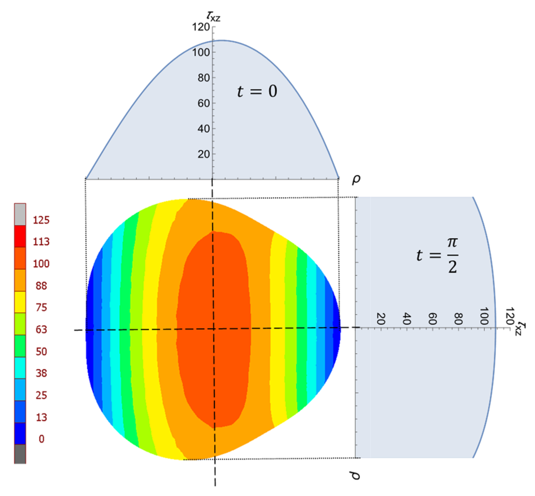
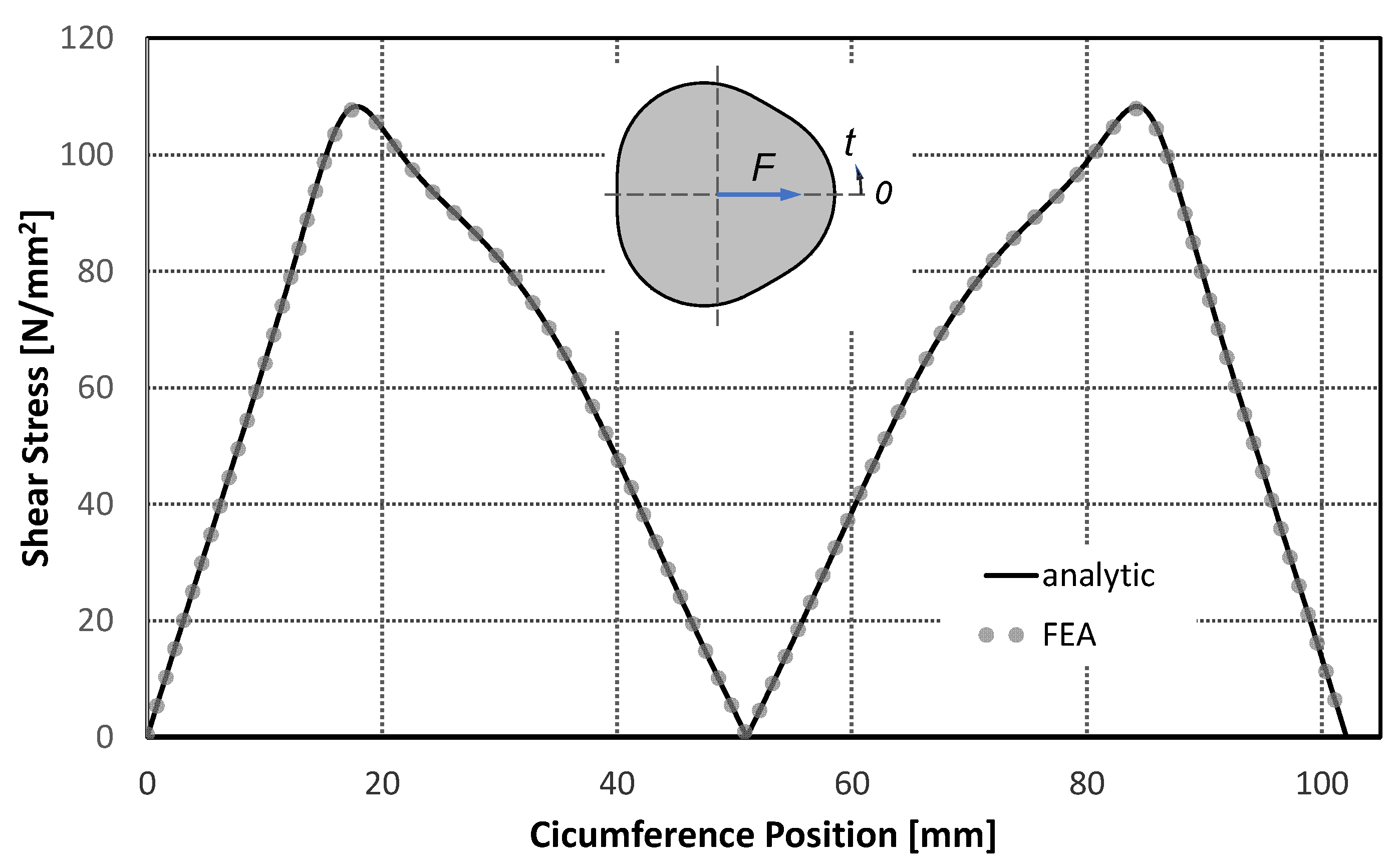
2.4. Shear Force Bending and Formulation
The general formulation for shear force bending is presented in [24,25] based on the elasticity behavior of the material. The method is described in more detail in [21], but a corresponding practical application is complex, as four stress functions must first be determined as a function of the profile contour. The method is, therefore, no longer suitable for practical applications. In contrast, the procedure described in [24] is presented in a more compact form. However, this also requires a complex bending stress as a function of the profile geometry. Based on the latter formulation, a general procedure was developed in the present work from a parametric profile description, according to Equations (3) and (4). The application was demonstrated in more detail using several test examples.
To analyze the transverse shear stresses, the origin of the coordinate is placed in the center of gravity of the profile surface, as shown in Figure 10. Force F is applied on the right side at the center of the cross-section and in the -direction.
Figure 10.
Definition of the coordinate system.
At any axial point at distance from the coordinate origin , the resulting bending moment in relation to the -axis is as follows:
where is the length of the beam. However, in the case of shear force bending, and no longer disappear, as the shear force causes a shear stress on the cross-section. The following equations are, hence, valid:
If we insert these values into the equilibrium conditions, we obtain
The first two parts of the equation mean that and are not dependent on .
For the further procedure, a complex stress function for bending is required, which satisfies the corresponding compatibility conditions of the deformations as well as the boundary conditions (load-free profile contour). It has the following general form:
where describes the real and the imaginary part of the -function. Both functions are dependent on the contour geometry of the profile (e.g., Equations (1) and (3)). If the variable of is transformed into ζ, Equation (5) can be presented as follows:
Here, and are conjugate to each other, i.e.,
is labeled as a bending stress function. If a conformal mapping for transforming the unit circle on the cross-sectional area is available (Figure 11), a solution of for the entire profile cross-section can be determined from the boundary condition for on the profile contour. If it is not possible to derive a conformal map directly from the contour equations, the successive methods in [26] can be used to approximate a proper mapping function. The corresponding procedure is described in more detail below using an example.
Figure 11.
Illustration of the conformal mapping of the unit circle () on the cross-sectional area, which is exemplary for an epitrochoid with four sides ().
The boundary condition on the profile contour, can be derived as follows [24]:
Due to the closed profile contour, the constant value on the right side of Equation (8) disappears. If the function is known, or can be determined using Cauchy’s integral formula.
Procedure for Determining
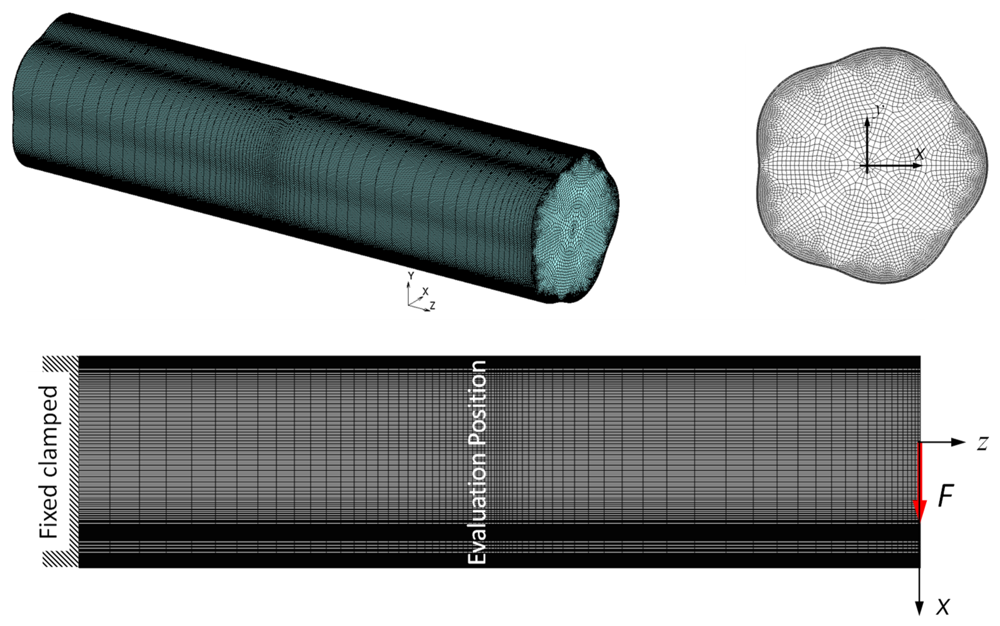
If the contour geometry has been described by parametric equations with “cos” and “sin” terms (e.g., Equation (1) or (3)), the cos and sin functions are first rewritten as expressions of :
where e is the Euler number. If these expressions are inserted into the parametric equations, the variables and can be represented as functions of . is the edge of the unit circle and corresponds to the profile contour in the real plane. Based on this, Equation (8) is represented as follows:
This can be used to determine or using Cauchy’s integral formula:
and are the real and imaginary parts of the complex bending stress function in the so-called model or ζ plane. The stress components can be determined using Equations (4) and (5) as follows:
For the partial derivatives of occurring in Equation (21), is also required:
where , and denote the corresponding derivatives according to parameter .
is the moment of inertia around the -axis and can be determined from the following relationship according to [22]:
The deformations can then also be determined as follows [19]:
The displacement in the z-direction (the 3rd equation in (24)) consists of a -dependent component, , which represents the rotation of the cross-section (Equation (25)), and a warping, , which is caused by the distribution of the shear stress. is independent of and can be determined from Equation (26):
The deflection is obtained from the first equation in (24), where and are equal to zero:
In the following, the procedures are first applied to the circular cross-section as a well-known classic example, and the results are compared with the solutions known from the technical literature. Then, the epitrochoidal profile cross-sections are also investigated.
3. Applications
To establish a basis for checking the analytical results, in addition numerical investigations were carried out by means of the finite element analysis (FEA), in which the results for some examples were compared with the analytical results.
Numerical models
For the numerical investigations, as in [23], the MSC-Marc program system was used. Figure 12 shows the mesh structure and the corresponding boundary conditions exemplary for an epitrochoidal cross-section with five sides. The profiled shaft is fixed on the left side. The shear force is transferred to the shaft’s right side via a reference node using RBE2 (Rigid Body Element, Form 2). The shear stresses were evaluated in the middle of the bar with a proper distance to the boundaries. To ensure that the results on the profile cross-section were as accurate as possible, the surface of the profile was meshed sufficiently fine and uniformly. The limit was determined by a convergence study on the FE model. The FE mesh in Figure 12 contains 504,430 hexahedral elements with full integration, type 7 according to the Marc Element Library [27], and 535,094 nodes.
Figure 12.
FE mesh and boundary conditions for the E-profile with five sides.
The FE meshes were generated with the help of software written in Python 3 language at the Chair of Machine Elements at the West Saxon University of Zwickau. The FE meshes were then transferred to the MSC-Marc program system and integrated into the pre-processing.
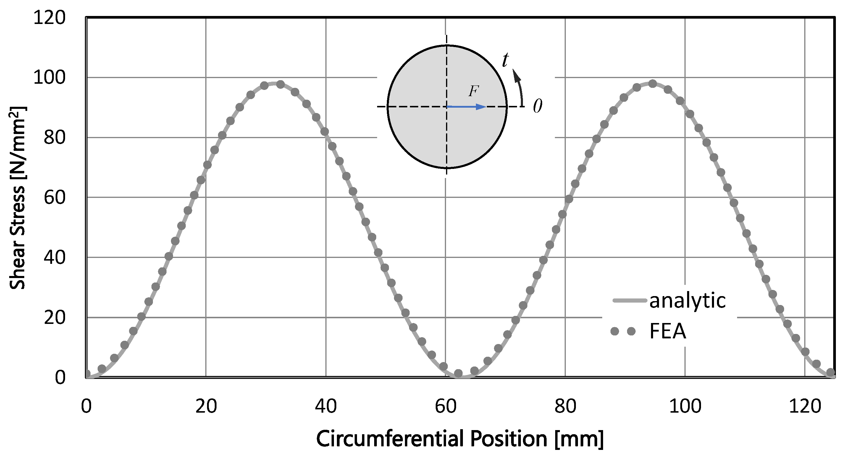
3.1. Circular Cross-Section
The following conformal mapping applies to a circular cross-section:
This function forms the unit circle conformally and completely on the cross-section of the shaft. The contour edge can be described as parametric:
If Equation (18) is inserted into (29) and the results for and are inserted into Equation (19), the function for the contour can be obtained. Based on this, the complex stress function is determined from Equation (20). If is inserted into , the real part can be determined as follows:
Here, assumes values between 0 and 1. Substitute from Equation (30) into Equation (21) and replace and with the following relationships:
Thus, the equations for the shear stress components are obtained:
The resulting shear stress can then be determined as the vectorial sum of the two components:
With , the shear stress components can be determined as follows:
The stress distribution on the cross-section is shown in Figure 13. This is the result of the shear stress component from the numerical investigations (FEA) for a round cross-section with mm and . The material chosen for the shaft was steel with and a Poisson’s ratio of . According to Equation (32), the analytical solutions for the two-parameter angle positions and are also shown, where the agreement of the results can be traced by observing the color scale.
Figure 13.
Distribution of the shear stress component on a circular cross-section from FEA and Equation (32).
A more concrete comparison can be made using the stress distributions on the lateral surface, where applies. If is inserted into Equations (32)–(34), the following relationships are obtained:
The resulting shear stress can be determined from (34) as follows:
Figure 14 shows the course of on the contour of the cross-section. A very good agreement between the numerical results and the analytical solution—according to Equation (37)—can be seen from the figure.
Figure 14.
Distribution of the shear stress component on the round profile contour from FEA and Equation (37).
The maximum stress of the contour occurs at and can be determined according to the following equation:
The maximum shear stress occurs at the center of the cross-section (0, 0). At , is maximum and = 0; therefore,
For a Poisson’s ratio of (steel), the maximum shear stress at the center point can be determined from Equation (41), and the maximum shear stress on the profile outline from Equation (40) is as follows:
Compared with existing solutions
The solution for circular cross-sections known from the literature is based on the formulation of the classical theory of elasticity, which always depends on finding a suitable real shear function. This shear function should satisfy the corresponding equilibrium and compatibility conditions depending on the profile geometry. Therefore, solutions are only available for some specific profile geometries such as a circle, ellipse, or quadrilateral. Timoshenko [28] presents such a solution for the circular cross-section. Here, a real stress function is given in Cartesian coordinates, which leads to the same results from Equations (32) and (33):
is here the radius of the cross-section. The same results from (42) and (43) are obtained in [28].
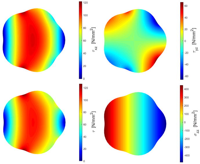
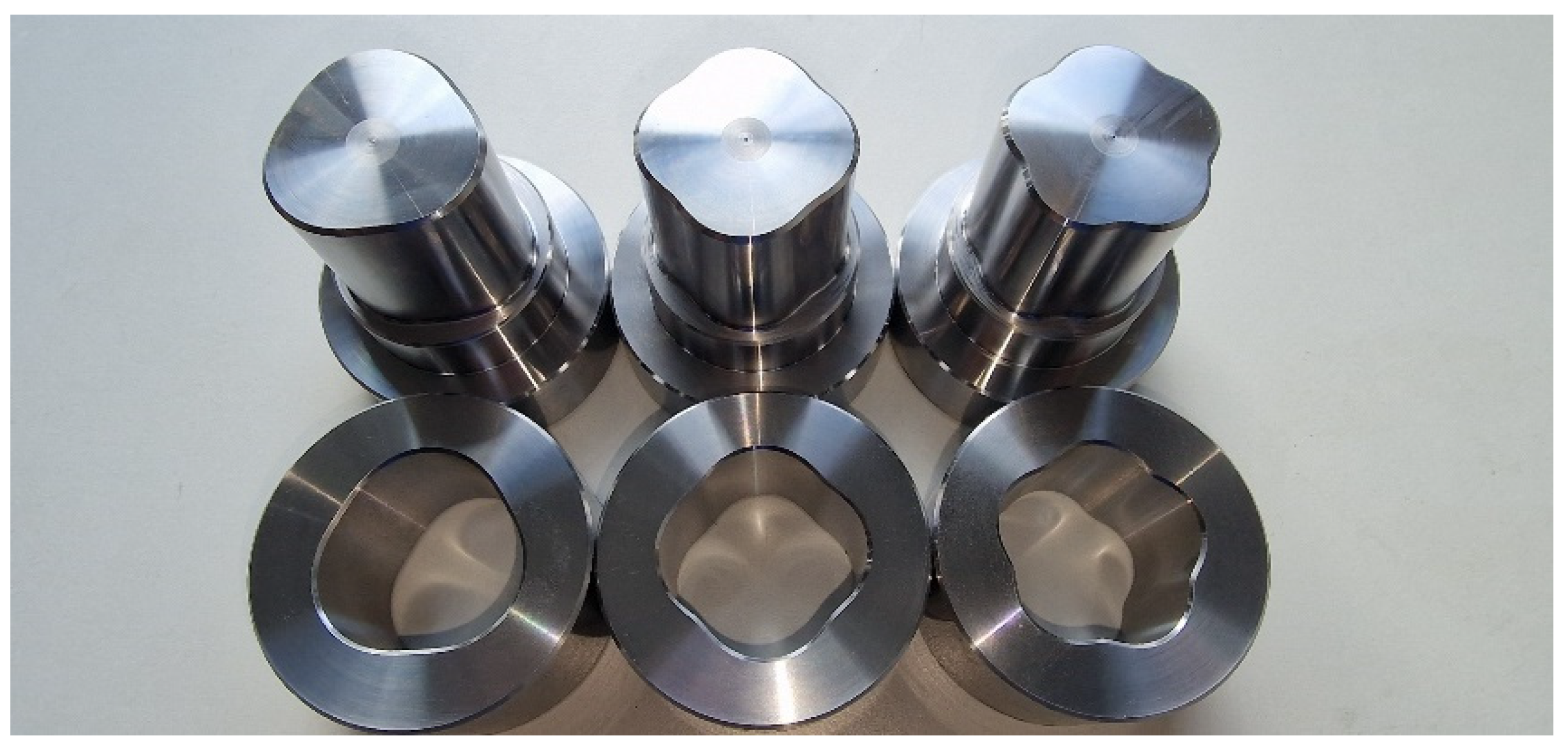
3.2. Epitrochoidal Profile Cross-Sections
For the epitrochoidal cross-section, the conformal mapping, according to Equation (2), applies, where is the number of sides of the profile. This function maps the unit circle conformally and completely on the profile cross-section (see Figure 11). This guarantees the solution over the entire profile cross-section according to Equation (20). In the following, is replaced by because there is only one eccentricity.
The contour in Equation (1) can be rewritten as follows (see Equation (18)):
Substituting Equation (45) into Equation (19) gives the function for the profile contour. Based on this, the complex stress function can be determined from Equation (20) using Cauchy’s integral Formula (20). If is inserted into , the real part of the stress function can be determined. Substituting into Equation (21) and replacing and with the following relations for the entire profile cross-section yields
The components of the shear stresses can be determined for the entire profile cross-section. Here, takes values between 0 and 1 ().
Because of the size of the equation, the general solution is not shown here. This can be found in the Appendix A.
In the following, two application examples for (Figure 1 in the left side) and n = 5 (Figure 1 in the right side) are presented, and the results are compared with the FE analysis.
Example 1.
with flat flanks.
For an epitrochoid with three sides, the following mapping function applies, which conformally transforms the unit circle on the epitrochoid:
If is inserted into Equation (44), the epitrochoid with three flat point flanks is obtained:
Figure 15 shows the iso- and lines for this profile with .
Figure 15.
and -constant lines for the epitrochoid with and , according to Equation (48).
If and are inserted into Equation (A4) in the Appendix A, the following relationship is obtained for the stress function:
If is also used for steel, the following function for the distribution of the shear stress component on the profile cross-section is obtained from (A6):
Furthermore, the following equation for the shear stress component results from (A7):
Figure 16 shows the distribution of the shear stress from the numerical FE investigations for the epitrochoidal cross-section with , mm, ( mm), and kN (for a load). The material chosen for the bar was steel with and a Poisson’s ratio of . Analytical solutions according to Equation (48) for the two-parameter angle positions of and are also shown, where the agreement of the results can be traced by observing the color scale.
Figure 16.
Distribution of the shear stress component on the epitrochoidal cross-section with from FEA and Equation (50).
To determine the resulting shear stresses on the profile outline, is used in Equations (50) and (51). Equation (34) is used to obtain the following relationship for the total stress distribution on the contour of the shaft:
A comparison of Equation (52) with the numerical results is shown in Figure 17, where very good agreement can be recognized.
Figure 17.
Distribution of the total shear stress on the epitrochoidal profile contour with from FEA and Equation (52).
Maximum shear stress occurs at the center point of the cross-section :
Example 2.
.
For an epitrochoid with five sides, the following mapping function applies, which can conformally transform the unit circle on the epitrochoid area:
Figure 18 shows this profile for this example with . The iso- and lines are shown in the figure.
Figure 18.
- and -constant lines for the epitrochoid with and , according to Equation (54).
If and are inserted into Equation (A4), the following relationship is obtained for the stress function:
Furthermore, Equation (A5) yields the following relationship for :
Consequently, the following equation for the shear stress component on the profile cross-section can be obtained for (steel) from (A6):
Furthermore, the following relation follows from (A7) for :
Figure 19a shows the distribution of the shear stress components from the numerical FE investigations for the epitrochoidal cross-section with , mm, ( mm). A shear force of was applied, and the chosen material was steel with and a Poisson’s ratio of . Analytical solutions according to Equation (57) for the three-parameter angle positions , , and are also shown, where the agreement of the results can be identified using the color scale. The visualization of Equation (57) was carried out using a MATLAB [29] script. The outcome is shown in Figure 19b, where the agreement with the FEA result (on the left) can be recognized. The MATLAB script can be found in Appendix B with some more examples.
Figure 19.
Distribution of the shear stress on a five-sided epitrochoidal cross-section from FEA and Equation (57) (a), and Visualization of Equation (55) by using a MATLAB script (b).
The total shear stress is the vectorial sum of the two components according to Equations (57) and (58). Figure 20 shows the distribution of the resulting shear stresses over different -lines.
Figure 20.
Distribution of the resulting shear stress for different -lines on the epitrochoidal cross-section.
The shear stresses on the profile contour correspond to . This fact leads to the following equation for the distribution of the shear stress on the profile contour with :
The following then applies to the investigation case with and :
Equation (58) represents the curve with in Figure 19.
3.3. Bending Stress According to [20]
For the general case of bending stress, according to [20], the following relationship can be determined for the bending stress due to a shear force:
Here, denotes the angle of rotation of the shear force, , around the -axis. Variable accepts the value 0 for the center point (neutral axis) and the value 1 for the outer profile contour. Figure 21 shows the distribution of the bending stress, according to Equation (61), for different -lines.
Figure 21.
Distribution of the bending stress on the profile cross-section for different -lines.
3.4. Deformations
The deformations of the profile cross-section can be determined from (24) as functions of and with the known stress function . The results for the three displacement components in curvilinear coordinates are summarized in the Appendix A. If is inserted into Equations (A9)–(A11), the following equations are obtained for the deformation components:
The deflection, i.e., the deformation of the neutral axis, is determined from Equation (62) at (or from the first equation of (24) at ) as follows:
Figure 22 compares Equation (65) with the results of the FEA, where a good match can be recognized.
Figure 22.
Deflection according to Equation (65) compared with the FEA results.
4. Conclusions
This article deals with an analytical approach to determining the distribution of the shear stresses on non-circular profile cross-sections due to shear forces. The solution completes the existing analytical attempts at the load cases of pure bending and torsion. The approach was developed based on the complex theory of elasticity with the aid of conformal mapping, where solutions to the stress components can be derived in Cartesian, as well as in a curvilinear coordinate system corresponding to the contour geometry. The developed method was first applied to a round profile cross-section, and the results were compared to the solutions known from the literature, where a complete agreement was observed. Furthermore, two epitrochoidal profiles with three and five flanks were examined. The analytical stress results show very good agreement with the numerical investigations from FEA. The elastic deformation components were also determined for the examples. An equation for the deflection was derived from , for which very good agreement with the FEA was also observed. The obtained equations allow a quick design of the profiled shaft with the help of a simple pocket calculator without expensive FE analyses. The equations derived for the general case with flanks and an arbitrary eccentricity are put together in an Appendix A for both the stresses and the deformations. A MATLAB script was also written to enable visualization of the stress distributions on the profile cross-section, which is presented in a further Appendix B.
Funding
This research received no external funding.
Institutional Review Board Statement
Not applicable.
Informed Consent Statement
Not applicable.
Data Availability Statement
The original contributions presented in the study are included in the article, further inquiries can be directed to the corresponding author.
Acknowledgments
This work is dedicated to my doctoral supervisor Franz Gustav Kollmann on the occasion of his 90th birthday last August. The author wishes him good health and many more lucky years.
Conflicts of Interest
The author declares no conflict of interest.
Nomenclature
| Formula symbols: | ||
| mm2 | Area of profile cross-section | |
| e | mm | Profile eccentricity |
| e | - | Euler’s number |
| E | MPa | Young’s modulus |
| F | N | Shear force |
| mm | Deflection | |
| Torsiol stress function in the polygon coordinate system | ||
| Bending stress function in the polygon coordinate system | ||
| Bending stress function in the Cartesian coordinate system | ||
| , | mm4 | Area moment of inertia in the Cartesian coordinate system |
| l | mm | Length of profile shaft |
| Nm | Bending moment | |
| n | - | Profile periodicity (number of sides) |
| mm3 | First moment of area | |
| r | mm | Nominal or mean radius |
| t | - | Profile parameter angle |
| mm | Displacement components | |
| x, y, z | mm | Cartesian coordinates |
| Complex function of polygon contour | ||
| Greek formula symbols: | ||
| - | Relative eccentricity | |
| Rotation angle of the coordinate system | ||
| Real stress function in Cartesian coordinate system | ||
| - | Physical plane unit circle | |
| Poisson’s ratio | ||
| Real part of torsion function in polygon coordinate system | ||
| Real part of stress function in Cartesian coordinate system | ||
| Real part of stress function in polygon coordinate system | ||
| Imaginary part of torsion function in polygon coordinate system | ||
| Imaginary part of stress function in Cartesian coordinate system | ||
| Imaginary part of stress function in polygon coordinate system | ||
| Curvilinear polygonal coordinates | ||
| MPa | Bending stress (z-component of stress vector) | |
| MPa | Shear stress components | |
| MPa | Total shear stress | |
| - | Coformal mapping function | |
| - | Complex variable in model plane | |
Appendix A
Mapping function for “simple” epitrochoids:
Surface area:
Area moment of inertia:
Real part of the stress function:
Imaginary part of the stress function:
Stress component: :
Stress component: :
Bending stress:
Displacement in the x-direction:
Displacement in the y-direction:
Displacement in the z-direction:
Deflection:
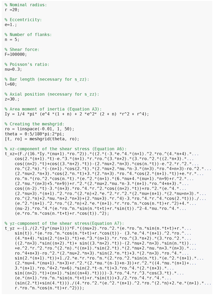
Appendix B. MATLAB Code for Visualization of the Stresses


The following applies: r = 20 mm, n = 5, e = 1 mm, nu = 0.3, and F = 100,000 N.

References
- DIN 5480-2:2015-03; Passverzahnungen mit Evolventenflanken und Bezugsdurchmesser—Teil 2: Nennmaße und Prüfmaße. DIN-Deutsches Institut für Normung e.V.: Berlin, Germany, 2015.
- Ziaei, M.; Selzer, M.; Sommer, S. Influence of a Shaft Shoulder on the Torsional Load-Bearing Behaviour of Trochoidal Profile Contours as Positive Shaft–Hub Connections. Eng 2024, 5, 834–850. [Google Scholar] [CrossRef]
- Selzer, M.; Ziaei, M.; Forbrieg, F. Einblick in die Festigkeitsberechnung nach DIN 3689 genormter hypotrochoidischer Welle-Nabe-Verbindungen unter reiner Torsionsbeanspruchung, Forschung im Ingenieurwesen. Forsch Ingenieurwes 2024, 88, 20. [Google Scholar] [CrossRef]
- Maximov, J.T.; Hristov, H. Machining of Hypocycloidal Surfaces by Adding Rotations around Parallel Axes, Part I: Kinematics of the Method and Rational Field of Application. Trakya Univ. J. Sci. 2005, 6, 1–11. [Google Scholar]
- Iprotec GmbH. Polygonverbindungen. Available online: www.iprotec.de (accessed on 22 October 2024).
- DIN 3689-1:2021-11; Shaft to Collar Connection—Hypotrochoidal H-Profiles—Part 1: Geometry and Dimensions. Beuth-Verlag: Berlin, Germany, 2021.
- Knabner, D.; Suchy, L.; Radtke, S.; Leidich, E.; Hasse, A. Fretting fatigue of cast iron and aluminium—A strength assessment method based on a worst-case assumption. Int. J. Fatigue 2024, 182, 108209. [Google Scholar] [CrossRef]
- Selzer, M.; Ziaei, M.; Brůžek, B. Optimierung der Hybriden Trochoiden für Serientaugliche Fertigungstechnologien auf Grundlage einer reinen Torsionsbeanspruchung. In Proceedings of the 10. VDI-Fachtagung “Welle-Nabe-Verbindungen”, Garching bei München, Germany, 6–7 November 2024. Contribution has already been accepted. [Google Scholar]
- Spura, C.; Fleischer, B.; Wittel, H.; Jannasch, D. Roloff/Matek Maschinenelemente Springer Fachmedien Wiesbaden, Normung, Berechnung, Gestaltung, 26th ed.; Springer Vieweg: Wiesbaden, Germany, 2023. [Google Scholar]
- Hagedorn, P. Technische Mechanik/Festigkeitslehre, 4., überarbeitete Auflage, Frankfurt am Main; Harri Deutsch Verlag: Thun, Switzerland, 2006. [Google Scholar]
- Dmitrii Ivanovich Zhuravskii. Available online: https://en.wikipedia.org/wiki/Dmitrii_Ivanovich_Zhuravskii (accessed on 18 October 2024).
- Hibbeler, R.C. Mechanics of Material, 8th ed.; Pearson, Prentice Hall: Hoboken, NJ, USA, 2011. [Google Scholar]
- Kharlab, V.D. On Elementary Theory of Tangent Stresses at Simple Bending of Beams. Procedia Struct. Integr. 2017, 6, 286–291. [Google Scholar] [CrossRef]
- Zwikker, C. The Advanced Geometry of Plane Curves and Their Applications, Dover Books on Advanced Mathematics; Courier Corporation: Chelmsford, MA, USA, 1963. [Google Scholar]
- Wunderlich, W. Ebene Kinematik; Bibliographisches Institut: Mannheim, Germany, 1968. [Google Scholar]
- Ziaei, M. Optimale Welle-Nabe-Verbindung mit mehrfachzyklischen Profilen, 5; VDI-Fachtagung “Welle-Nabe-Verbindungen”: Nürtingen, Germany, 2012. [Google Scholar]
- Frank, A.; Pflanzl, M.; Mayer, R. Vom K-Profil und Polygonprofil zu funktionsoptimierten Unrundprofilen—Eine österreichische Entwicklung. Fert. Präzision Spieg. 1992, 3, 42–48. [Google Scholar]
- Musyl, R. Die kinematische Entwicklung der Polygonkurve aus dem K-Profil. Wärmewirtschaft 1955, 10, 18–22. [Google Scholar]
- DIN 32711; Welle-Nabe-Verbindung—Polygonprofil P3G, Teil 1. Deutsches Institut für Normung e.V.: Berlin, Germany, 2009.
- Ziaei, M. Bending Stresses and Deformations in Prismatic Profiled Shafts with Noncircular Contours Based on Higher Hybrid Trochoids. Appl. Mech. 2022, 3, 1063–1079. [Google Scholar] [CrossRef]
- Ziaei, M. Analytische Untersuchung unrunder Profilfamilien und numerische Optimierung genormter Polygonprofile für Welle-Nabe-Verbindungen. Postdoctoral Thesis, Technische Universität Chemnitz, Chemnitz, Germany, 2002. [Google Scholar]
- Ziaei, M. Torsionsspannungen in Prismatischen, Unrunden Profilwellen mit Trochoidischen Konturen. Forsch. Ingenieurwesen 2021, 85, 985–995. [Google Scholar] [CrossRef]
- Ziaei, M. Bending and Torsional Stress Factors in Hypotrochoidal H-Profiled Shafts Standardised According to DIN 3689-1. Eng 2023, 4, 829–842. [Google Scholar] [CrossRef]
- Muskelishvili, N.I. Some Basic Problems of the Mathematical Theory of Elasticity; Springer: Dordrecht, The Netherlands, 1977. [Google Scholar]
- Sokolnikoff, I.S. Mathematical Theory of Elasticity; Robert E. Krieger Publishing Company: Malaba, FL, USA, 1983. [Google Scholar]
- Kantorovich, L.V.; Krylov, V.I. Approximate Methods of Higher Analysis; Translation Edition; Dover Publications: Dover, UK; Mineola, NY, USA, 2018. [Google Scholar]
- MSC Software Corporation. Marc 2020 Manual; Volume B (Element Library); MSC Software Corporation: Newport Beach, CA, USA, 2020. [Google Scholar]
- Timoshenko, S.P.; Goodier, J.N. Theory of Elasticity; McGraw-Hill Book Company: New York, NY, USA, 1985. [Google Scholar]
- MATLAB The MathWorks, Inc. MATLAB Version: 9.13.0 (R2022b). 2023. Available online: https://www.mathworks.com (accessed on 1 January 2023).
Disclaimer/Publisher’s Note: The statements, opinions and data contained in all publications are solely those of the individual author(s) and contributor(s) and not of MDPI and/or the editor(s). MDPI and/or the editor(s) disclaim responsibility for any injury to people or property resulting from any ideas, methods, instructions or products referred to in the content. |
© 2024 by the author. Licensee MDPI, Basel, Switzerland. This article is an open access article distributed under the terms and conditions of the Creative Commons Attribution (CC BY) license (https://creativecommons.org/licenses/by/4.0/).