Abstract
This study focusses on a method for estimating the urban recharge and evaluating the ground water quality for drinking and irrigation purposes. The study was carried out in the Liverpool Local Government Area of New South Wales, Australia, and it included year-long monitoring of four boreholes for the water table depth and water quality. Average depth of water table was in the range of 1 to 4 m from the land surface. The pattern of variations in the water table depth (WTD) varied across the four boreholes. The WTD variations between borehole 2 (BH2) and borehole 3 (BH3) were similar, but significantly different variations were exhibited in BH1 and BH 4, with BH1 showing a quicker response to rainfall events. The presence of lake appears to have influenced the recharge pattern in the adjacent area as reflected in the WTD variations in BH3 and BH4. The recharge rates for BH3 and BH4 was about 2 to 5 times higher than those observed for BH1 and BH2, which are located at a relatively greater distance from the lake. This indicates that the presence of urban lakes can influence recharge rate in the area. Water quality analysis indicated higher salt and turbidity levels, which may be attributed to the local geology (the Wianamatta group) present in the study area and/or possible saltwater intrusion. This has implications for the treatment cost associated with the supply of the groundwater for drinking and irrigation purposes. Pearson’s analysis indicated a significant correlation between EC, TDS, Turbidity and pH. The turbidity of groundwater varied between 33 and 530 NTU, indicating that the turbidity may have been affected by the dissolution of salt deposits via colloidal particles. Significant variations in groundwater quality during rainy periods, also, indicated the existence of groundwater recharge in the study area. This study highlights the issues associated with the groundwater recharge and quality management in urban landscapes and provides a basis for further research.
1. Introduction
1.1. Importance of Groundwater
Groundwater plays an important role in the urban society and rural environment, as it is used for agricultural, drinking and industrial purposes [1]. Groundwater plays three key roles in our environment: it provides base flow, which helps to keep most rivers flowing all year long, acts as a source for maintaining good river water quality by providing dilution to sewage and effluent discharges, and as an important source of water supply [2,3]. About half of the world’s urban population depends on groundwater as the major source of water supply [4], and its effective management is becoming critical in meeting urban water needs [5]. The urban aquifers are crucial to the long-term viability of many cities around the world [6]. However, land use changes, urban development or urbanisation may result in either increases or decreases in groundwater recharge [7].
There are negative consequences associated with uncontrolled use of groundwater such as aquifer depletion, water quality degradation [8], land subsidence [5,9], soil erosion [10] and saltwater intrusion from coastal areas. The two major threats to groundwater use are over-exploitation and increase in the pollution [11]. Both human and natural activities tend to impact the quality of groundwater and recharge [4,12,13,14,15]. The urban system is complex, and contamination can emanate from multitude of point sources that are widespread and diffuse, such that it becomes difficult to predict the exact source of contamination [4,6,16]. Cases abound where development of groundwater is carried out without adequate understanding of recharge and the relationship between the exploited aquifer and water sources. The implication of this act is that it leads to over-allocation and over-exploitation with its attendant consequences [17].
1.2. Estimation of Recharge
The estimation of recharge in an urban environment is more complex than in a rural setting due to a range of land uses and variation in recharge areas in the landscape. The urban environment is characterised by abundance of dense network of drainage channels, water supply networks and drains that carry away stormwater and sewage. Any leakages in these networks can add to the recharge of groundwater and these numerous pathways associated with urban environment make it difficult to quantify the recharge. Hence, various sources of recharge such as pathways for precipitation and routes for water supply and sewage should be identified prior to estimation of urban recharge [4,18]. The traditional method used to estimate urban recharge is a combination of water balance with groundwater modelling. However, due to the complexity of the urban environment, most studies do not consider all the sources and routes of recharge [19].
Flow through the unsaturated zone is mainly through the matrix, fissures, or a combination of both pathways. Matrix pore flow is very slow as a result of its low hydraulic conductivity and high porosity. Recharge delivery by fissure flow is more pronounced when the water table is shallow [20]. The time and intensity of groundwater recharge is influenced by fissures due to the alteration of the soil storage capacity and the infiltration processes. The rate of vertical infiltration is increased by fissures, which lead to increase rate of groundwater recharge. However, it can also lead to increased rate of drainage [21].
Several studies have been reported related to different methods used in recharge estimation such as the Water Table Fluctuation (WTF) [13,22,23,24], the water balance method [20], the chloride mass balance method [25] and the numerical modelling [26]. In some instances, a combination of methods has been used to estimate the recharge which yielded different outcomes. In the case of WTF method, specific yield has been determined by pumping test, aquifer tests, water-budget methods, water table response to recharge, field test, and laboratory method. The specific yield value, which is necessary in the computation of groundwater recharge by WTF method, varies greatly due to variations in geology and depth to water table [3].
Most studies on recharge estimation via WTF have not properly accounted for lateral flow and runoff [13,22,24,27]. Oliveira et al. [13] used WTF to evaluate the impact of land use and land cover on recharge estimate of Brazilian savannah. The mean value of laboratory determined specific yield (Sy) from research in the catchment was used to compute recharge. Crosbie, Binning and Kalma [23] adopted a modified time series WTF method by incorporating varying Sy with respect to depth to estimate groundwater recharge. The result was that groundwater recharge estimated using a constant Sy exceeds that obtained with varying Sy. Cai and Ofterdinger [24] used a similar time series WTF method but with a constant Sy to estimate annual recharge. Varni et al. [27] used the graphical method of fitting eighteen years record of rainfall values against water table rises to determine Sy and estimated the monthly and annual recharge which were similar with literature values of the area. Scanlon et al. [14] suggested that WTF method is a good tool to estimate recharge rates in areas not under severe impact of pumping.
1.3. Importance of Groundwater for Australia
The importance of groundwater in Australia cannot be overstated, as it is the driest inhabited continent on Earth and where surface-water resources are limited over large areas. It is estimated that the total water consumption in Australia is about 15,000 GL per annum and one-third of it is sourced from groundwater and the rest from surface-water sources [28]. Due to the severe drought recorded in many parts of New South Wales (NSW), extraction of groundwater has been identified as a viable drought response option that can help to secure and prolong Sydney’s water supply [29]. Many urban, rural and remote communities around Australia depend on groundwater resources to satisfy their water needs. Drinking water guideline values, are determined based on the impact of chemical components considered to pose a great health risk to humans at concentrations above the specified limits. It is imperative that public water supplies do not exceed the guideline values, and consumers are now more aware of the adverse health effect of drinking water polluted by toxic metals [30].
1.4. Objectives
In the current study, a micro level investigation was carried out in Wattle Grove area of New South Wales, Australia to estimate the daily groundwater recharge. Given that the urban catchment considered in this study is not affected by the extraction of groundwater, it was decided to use water table fluctuation (WTF) method to estimate the groundwater recharge. Additionally, the urban area considered is relatively new development (developed in 1990s [31]). As such, no leakage is expected from both water supply and wastewater collections systems. In this study, a heuristic method was used to estimate the lateral flow, which is then used to estimate the groundwater recharge. Hydrochemical analysis has been carried out to understand the suitability of the groundwater for the irrigation and drinking purposes. A systematic sampling, analyses and interpretation approach was adopted for the primary and secondary hydrogeological and hydrochemical data. The outcome of this study may help to understand the influence of land use/landcover on the groundwater recharge in coastal urban areas.
2. Materials and Methodology
2.1. Study Area
The study area is located between 33°56′57.7″ S to 33°56′56.2″ S latitude and 150°56′25.4″ E to 150°56′22.6″ E longitude in Wattle Grove Sydney of New South Wales, Australia (Figure 1). It is about 36 km south-west of the Sydney Central Business District (CBD) and approximately 5 km from the Liverpool CBD. In the period 2013–2018, in Wattle Grove area, minimum annual rainfall was around 557 mm in 2018, while the highest annual rainfall of 989 mm was recorded in 2016 [32]. The study area is located in mild to cool temperate climatic zones. The study area comprises of a total catchment area of about 95 hectares, with approximately 1022 residential properties [33,34].
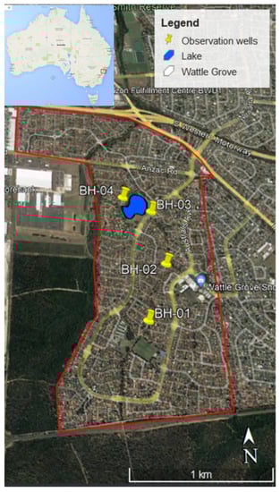
Figure 1.
Study area map showing borehole locations and Wattle Grove Lake (adopted from [35]).
2.2. Site Selection for Boreholes and Their Development
To determine the location of groundwater monitoring points, a literature review was conducted to find out information on geological and hydrogeological settings of areas surrounding the study area and available registered groundwater monitoring wells near Wattle Grove. Most of the registered wells (about 12) are situated on the north and north-west of the Wattle Grove Lake (WGL) but only one is situated on the south-east side of the lake. Four boreholes were identified based on reconnaissance survey, preliminary assessment of available topographical drawings and existing information on regional hydrogeology in literature (Figure 1). BH4 is located downstream of the lake and it is about 3 m from the edge of the lake. The other three (BH3, BH2 and BH1) are located at approximately 10 m, 500 m and 900 m upstream of the lake, respectively. The borewells were constructed using Sectional Flight Auger (SFA) method and were developed by using a Twister pump to empty their content which ensures maximum hydraulic connection between the bores and the formation. More details regarding the boreholes are given in Table 1. Soil classification of all boreholes indicated that they are in an alluvium zone (Section 3.2). Additionally, site investigations did not reveal any major groundwater recharge points.

Table 1.
Borehole locations and descriptions.
2.3. Hydrogeology
The study area is underlain by alluvial sands, silts and clays overlying shale of the Wianamatta Group and Hawkesbury Sandstone [36]. Groundwater can be inferred to be present in the alluvium and shale [37]. The alluvial deposits are characterised as shallow, discontinuous and relatively permeable [37,38]. Alluvial deposits have conductivity in the range of 10 m/day to 239 m/day. The thickness of aquifer in saturated zones of alluvium ranges from 3 to 17 m and increases downstream [38]. The result of hydraulic testing performed in the alluvium along Georges River shows that hydraulic conductivities range from 0.003 to 0.1 m/day [38].
The Wianamatta Group consists of three units namely the Ashfield Shale, the Minchinbury Sandstone and the Bringelly Shale, with the Minchinbury Sandstone of negligible thickness. The typical maximum thicknesses of this group are in the range of 100 to 150 m. The sedimentary rocks of Wianamatta Group have extreme low matrix porosity, and groundwater storage and transmission are achieved through secondary structures such as fracture and joints. The groundwater in the boreholes installed within the Wianamatta Group was generally found to be too saline (31,750 mg/L of TDS) [39].
The Hawkesbury sandstone is a dual porosity regional aquifer system found across the whole of the Sydney Basin. Groundwater flow is variable throughout the Hawkesbury sandstone and is generally dominated by secondary porosity and fracture flow such as faults and fracture zones [40]. Due to the poor transmitting capability of the Hawkesbury Sandstone, the local hydro-geological conditions may activate the aquifer as confined, unconfined or intermediate conditions. The hydraulic conductivities of Hawkesbury Sandstone have been reported to range from 0.5 m/day at the surface to 0.01 m/day at 50 m depth based on 370 packer tests conducted around the Sydney metropolitan area [41]. Figure 1 shows the geologic features of the aquifer in the study area and their associated thicknesses.
2.4. Soil Sampling and Analysis
The soil samples were collected at different depths (0–10 m) during drilling of the boreholes with sectional flight auger (SFA) method and stored in protective plastic bags. The samples were then transported to the soil laboratory located at Kingswood campus of Western Sydney University and preserved for specific retention analysis. The pressure plate method was used to determine the specific retention of the soil samples at different depths. The volumetric ring method was used to determine the soil bulk density which was then used to calculate the soil porosity. The sieve analysis was carried out according to AS 1289.3.6.3 [42].
2.5. Acquisition of Water Table Depths
To acquire the water table depth data, borewells were installed with data loggers. BH1 was instrumented with Levellogger edge™ and Barologger edge™ (Hydroterra, Melbourne, VIC, Australia) with the accuracy of ±0.05%. The Barologger edge was used to compensate for the variation in atmospheric pressure on water table measurement by Levellogger edge. On the other hand, BH2, BH3 and BH4 were monitored using Odyssey® depth and temperature data loggers (Odyssey, Christchurch, New Zealand). The resolution of Odyssey depth and temperature loggers at a depth of 10 m is approximately 2 mm. All the groundwater levels were logged at one-hour intervals from August 2017 to January 2019. The hourly rainfall measurements were obtained from the nearest weather observation station (Holsworthy Aerodrome AWS, 066161) [32].
2.6. Water Table Fluctuation Method
The water table fluctuation (WTF) method is a physical technique of calculating recharge. The WTF method relies on the fact that rises in groundwater levels in unconfined aquifers are due to recharge water arriving at the water table [22,26,43]. In the WTF method, groundwater recharge is estimated by the height of the water table build-up during/after a rainfall event, which is a change in water table height over the time interval multiplied by the specific yield [22,24]. The mathematical expression is:
where R is groundwater recharge (L/t), Sy is specific yield (dimensionless), and Δh (L) is change in water table height over the time interval Δt (t).
Equation (1) can be seen as a linear correlation between groundwater table rise and groundwater recharge with the coefficient (specific yield). The derivation of Equation (1) is under the assumption that water arriving at the water table goes completely into storage. The Sy is determined in the laboratory by applying the below equation:
where Sy is specific yield (dimensionless), is porosity (dimensionless), and is specific retention (dimensionless) which is determined by the pressure plate method. However, the Sy used in Equation (1) is the average specific yield (y), which is determined by the formula given by [44] Jinxi and Xunhong (2010) as:
where is the average specific yield value for the soil samples within total test depth at site i, is the value of specific yield for individual soil samples within interval depth of j at site i, and Li,j is the length of the soil samples within interval depth of j at site i. i refers to BH1, BH2, BH3 and BH4, while j refers to 0 m, 0.5 m, 1 m, …, 10 m.
To calculate the daily groundwater recharge, change in storage due to lateral flow during no or less rainfall was determined by taking the difference in WTD between the beginning and end of the months. This change in the storage was calculated for the months April 2018 and July 2018 when there were minimum rainy days in the study region (Table 2). Further, change in the storage were calculated for October and December 2018, when the rainfall amount was highest during the study period. These changes in storage could be attributed to both lateral flow as well as recharge due to rainfall. Monthly data was used in Table 2 as the daily groundwater level (GWL) fluctuations were too erratic. Inspection of Table 2 indicate that all the borewells are located on discharging aquifer with strong lateral flows.
Table 2.
Monthly differences in the WTD (− indicates WTD increase and + indicates WTD reduction).
Thus, the actual recharge is estimated using Equation (1), where ΔH/Δt is calculated using Equation (4).
Using Δh/Δt obtained from Equation (4), the recharge is estimated using Equation (1).
2.7. Water Samples Collection and Analysis
The groundwater samples were collected from the four newly developed monitoring wells from 7 August 2017 to 17 January 2019. The samples were collected monthly from each borehole using Twister pump (Hydroterra) connected to LDPE tube and powered with a 12 V battery. The samples were stored in sterilized polyethylene bottles (1 L) and transported to laboratory in ice cooler and stored at 4 °C for hydrochemical analyses. Before each sample collection, the bores were purged to ensure that stagnant water within the bores were removed and that the samples were obtained with minimum disturbance to the in situ geochemical and hydrogeological conditions [31]. On site readings such as EC, pH, and DO were monitored using portable HQ40d (HACH, Loveland, CO, USA) meter, while turbidity was measured with a portable 2100Q Turbidimeter (HACH, USA). Both meters were calibrated with recommended standard solutions prior to taking onsite readings. Ca, Fe, Mg, K and Na were analysed with inductively coupled plasma-optical emission spectroscopy (ICP-OES) (Agilent 700 Series).
To determine the groundwater quality for the irrigation purposes sodium percentage (% Na) and sodium adsorption ration (SAR) were analysed. The % Na was obtained using Equation (5):
where the ionic concentrations were expressed in meq/L.
SAR is obtained using the relationship between the major cations found in groundwater, namely, calcium, magnesium and sodium with the exception of potassium. It is expressed in milli equivalents. The formulae used to obtain SAR for each borehole is:
where the ion concentrations are expressed in meq/L.
The % Na is an indication of the soluble sodium content of the groundwater and used to evaluate Na hazard, whereas salinity hazard (SAR) is directly related to the quantity of salts dissolved in the irrigation water [10]. The diagram proposed by U. S. Salinity Laboratory [45] depending on sodium adsorption ratio (SAR) and EC, is used to affirm the suitability for irrigation applications.
3. Result and Discussion
3.1. Daily Groundwater-Level Fluctuations
The daily groundwater-level fluctuations of all four boreholes and daily rainfall data obtained from BOM site location number 066161 [32], over one year, is shown in Figure 2. The water table depth (WTD) from ground surface in BH1 could be described as having two major stages—an increasing stage until September and a gradually decreasing stage until the end January. The water table depth was highest in September compared with both the beginning and end of monitoring period. The end of water table depth is higher than the beginning of water table depth by about 219 mm. During dry season (May–September) the water table depth increased rapidly despite having some rainfall events which were of small magnitude. In the case of wet season, the water table depth showed a constant level between September and November and continued with a rapidly decreasing stage during many rainfall events with high magnitudes that occurred in the wet season. The annual variation of groundwater level is 594 mm. As shown in Figure 3, GWL variations were rapid and erratic. This may be attributed to the lateral groundwater flow conditions. No major recharge structures (such as leaking water and wastewater and large lake) or extraction facilities exist in the region. It can be said that the overall response of groundwater level to rainfall depicts a distinctive pattern for BH1 (Figure 3a) as the groundwater fluctuation exhibited smooth seasonal change.
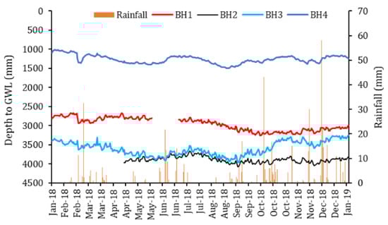
Figure 2.
Daily rainfall and groundwater-level fluctuations for all the borewells over the monitoring period.
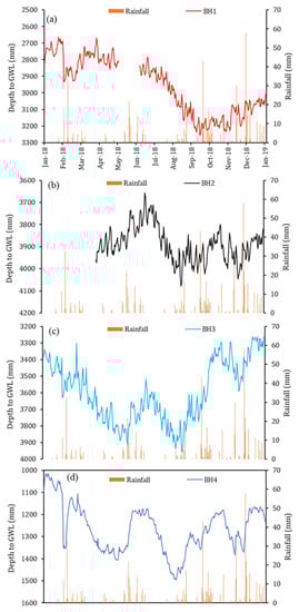
Figure 3.
Daily rainfall and daily groundwater-level data for (a) BH1 (b) BH2 (c) BH3 (d) BH4.
BH2 displayed one each of distinct WTD decreasing and increasing. There were few minor fluctuations, especially between August 2018 and January 2019. The main decreasing stage occurred in the period May–July. On the other hand, the main increasing stage occurred in the period July–September (Figure 3b). During the rainy period, there were large fluctuations in WTD. The gap (Figure 3b) at the beginning of BH2 groundwater fluctuation was due to the logger failure. The maximum water table depth was achieved in September. The rainfall events with high magnitude in the wet season only increased the water table depth between November to December while it decreased after that. As expected, the water table depth increased in the dry season (July–August). The difference between the beginning and end of monitoring was found to be very small (22 mm), while the difference between the maximum and minimum WTD was 421 mm over the monitoring period. BH2 showed some sharp changes in the WTD during the wet season (September–January). The observed drastic changes in WTD is an indication of rapid responses to individual rainfall events, which is linked to several hydro-geological parameters [24].
BH3 displayed one each of major increasing and decreasing WTD periods. Additionally, two each of minor increasing and decreasing WTD periods were observed. As expected, increasing WTD occurred during dry periods and decreasing occurred during wet periods. The WTD variation pattern appears to be different to BH2, which did not experience major decreasing or increasing periods. However, the increasing and decreasing periods appears to be similar to that of BH2. The highest water table depth was recorded in September (Figure 3c), which is similar to BH2. The water table decreased from September till the end but there were occasional increases in the wet season. The difference between the beginning of water table depth and end of water table depth is 61 mm. The annual water table variation is 729 mm.
BH4 exhibited two major increases in WTD, and they were followed by minor decreases. The WTD variations appear to be more erratic in the case of BH4. This can be attributed to the presence of lake adjacent to the monitoring borewell. The sudden increase followed by immediate decrease in WTD in February may be due to the error in the monitoring sensor. The highest water table depth (WTD) was recorded in August, which is the end of dry period. Generally, as expected, the water table depth decreased in the wet seasons. The final water table depth was about 352 mm less than the initial water table depth. Its annual water table variation was 452 mm.
Overall, the WTD fluctuations between all the boreholes varied from 0.4 to 0.8 m. BH3 has the highest annual water table variation followed by BH1 and BH4, while the least was BH2. The groundwater level observed across the four monitoring sites show that different hydrogeological regimes impact the groundwater flow and storage. The results appear to indicate no discernible trend in WTD variations. As seen in Figure 3, there were drastic fluctuations in the water table depths (WTD) on a daily basis. As shown in the figure, the WTD in BH2, BH3 and BH4 appears to vary quite rapidly, and the variation seems to be similar. Especially, the WTD in BH4 appears to be sensitive to rainfall event. This may be because BH4 is located next to the man-made Wattle Grove Lake (WGL). On the other hand, WTD in BH1 appears to be gradually increasing and then reducing during the high rainfall period.
In terms of rainfall pattern, in the beginning of the monitoring year, there was not much rain. Towards the later stages, there were high rainfall events (between October 2018 and February 2019). Since the daily fluctuations were quite unpredictable, average fluctuations over the month were calculated. These are shown in Table 2. As shown in the table, the difference in the WTD over each month for each of the boreholes are presented. The table also presents the combined average fluctuations against each of the months. Figure 4 presents a plot of monthly WTD fluctuations against the monthly rainfall for BH3. The figure indicates that there is a direct correlation between the change in the WTD and the amount of rainfall in the given month. Under low and no rainfall conditions, lateral flow appears to be predominant as a result, the groundwater level goes down. On the other hand, when the rainfall increases, the groundwater recharge becomes predominant and as a result its level increases. This observation applies to all the borewells and justifies the application of Equation (4) for calculating recharges for all the borewells.
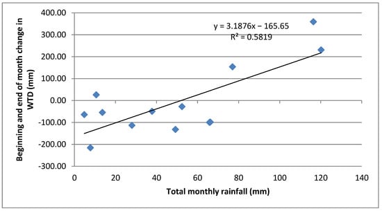
Figure 4.
Relationship between monthly WTD change and total rainfall for BH3.
3.2. Soil Classification
The results obtained from the sieve analysis and sedimentation tests were used to classify the soil samples according to Unified Soil Classification System (USCS) and United States Department of Agriculture (USDA) [46] textural soil classification. Figure 5 shows the combined soil profile at the four boreholes and the variation of the soil texture at different depths. The texture of the soil across the four monitoring sites at a depth of 0–1 m is generally made up of sand. All 4 boreholes exhibited similar soil profiles, except that BH3 and BH4 appear to contain larger sandy loamy layer. The top 10 m of the aquifer can be considered of alluvium type.
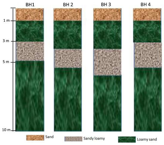
Figure 5.
Combined soil profile at BH1, BH2, BH3 and BH4 bores.
3.3. Specific Yield Estimation
Figure 6 shows the values of specific yield obtained from the four monitoring sites at different depths. As seen in the Figure 6, the specific yield generally varied between 25% and 45%. There was no trend in the variation of specific yield, except in the case of BH1. Most of the specific yield values for BH1 remained high. This could be attributed to variation of grain size, grain shape, sorting and compaction of sediments [44]. Average Sy values for the monitoring sites at BH1, BH2, BH3 and BH4 were 41%, 31%, 38% and 31%, respectively. It is difficult to make direct comparisons between the Sy values obtained in this study with those reported elsewhere in literature due to the differences in soil type, methods of soil collection, methods of Sy determination and geographical differences [47].
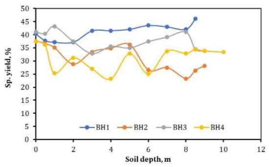
Figure 6.
Variation of specific yield with respect to depth.
3.4. Daily Groundwater Recharge Estimate
Using Equations (1)–(4), a computation table was set up to estimate the daily recharge. As discussed above, for BH1, BH3 and BH4, Δt values for no or less rainfall and high rainfall periods were 61 (April and July 2018) and 62 days (October and December 2018), respectively. For BH2, the corresponding Δt values were 31 and 62 days, respectively. The calculations are summarised in Table 3. As can be seen from the table, the daily recharge for each monitoring well was estimated as 5.23, 2.70, 1.77 and 1.37 mm/day at BH3, BH4, BH2 and BH1, respectively (Table 3). Both BH1 and BH2 daily recharge were below 2 mm/day. The low recharge obtained for BH1 and BH2 could be attributed to drier soils with higher moisture holding capacity or high surface runoff. During the dry season (May–September), there were several rainfall events that did not lead to an increase in the water table depth especially having thicker unsaturated zone. The recharge rates estimated for BH3 and BH4 were relatively higher than BH1 and BH2. This may be due to the presence of the Wattle Grove Lake (WGL) in the vicinity of BH3 and BH4. The impact of urban lakes on the groundwater recharge was also reported by other researchers [47,48]. Recharge values for BH3 and BH4 indicate that about 2 to 5 mm/day of infiltration may be expected due to the presence of the lake in the area. This can have some significance for managing the stormwater from the urban area.
Table 3.
Specific yield values and calculation of recharge.
3.5. Physico-Chemical Analysis of Borewell Water
Results of different physico-chemical analysis is presented in Table 4. The quality parameters of bore water was compared (Table 4) with other studies conducted within 25 km radius of the study area and drinking water quality standards [49,50,51]. Average pH values found for the groundwater in BH1, BH2, BH3 and BH4 were within the literature values observed around the study area. On average, the mean dissolved oxygen (DO) values found for the groundwater in all four boreholes exceeded the study areas range. The DO values observed in this study are generally higher and may indicate that there is active inflow of rainwater into the aquifer system. The average total dissolved solids (TDS) value of BH2 was below the catchment range while TDS values of both BH3 and BH4 were within the range. On the other hand, the average TDS value of BH1 far exceeded the range of values obtained for the study area by approximately 36%. The average concentration of Ca, K and Fe of all four boreholes were within the range of values reported for the catchment. In terms of the average concentrations of Mg and Na, only BH2, BH3 and BH4 were within the range reported for the study area while BH1 was outside the range. BH1 average electrical conductivity (EC) values exceeded the values reported for the study area by about 15%. Higher EC values observed for BH1 is an indication that the groundwater may have a saline source. The ionic dominance for freshwater is in the order of Na+ > Mg2+ > Ca+ > K+.
Table 4.
Groundwater quality results from this study and local study from the same catchment.
It should be noted that Denham Court, which is one of the closest sites to the Wattle Grove Lake, appears to show very high concentrations of cations, particularly for Na [49]. Additionally, this site showed very high TDS. On the other hand, the Glenlee Road and Menangle Park sites, which are bit farther away from Wattle Grove catchment, show significantly lower levels for TDS, Na, Fe and EC. In particular, groundwater in BH1 contained very high levels of Na and these values appeared to be similar to those observed for Denham Court site (Table 4).
Figure 7 and Figure 8 show the variation in the groundwater quality in all the four boreholes and the lake using box plots and timeseries graphs, respectively. As shown in the box plots (Figure 7), the variations in the cation concentrations appear to be significant particularly for BH1 and BH4, this may be attributed to lateral flow of groundwater due to existing hydro-geological conditions and recharge. While variation in the quality of BH4 groundwater may be attributed to the presence of lake, variation in BH1 groundwater quality may be to the hydro-geological conditions, saltwater intrusion or to the presence of some external contaminant sources. Close observation of Figure 8 indicates that during high rainfall periods, cation concentrations in the lake water appear to drop in comparison to that of groundwater. This reduction appears to be significant in the case of BH2, BH3 and BH4. This may be attributed to the recharge occurring due to the rainfall. Temporal variations as shown in Figure 8 appear to indicate both groundwater and lake water quality is affected by the rainy periods. This again indicate the recharge of groundwater during rainy periods which, in turn, influencing the groundwater quality.
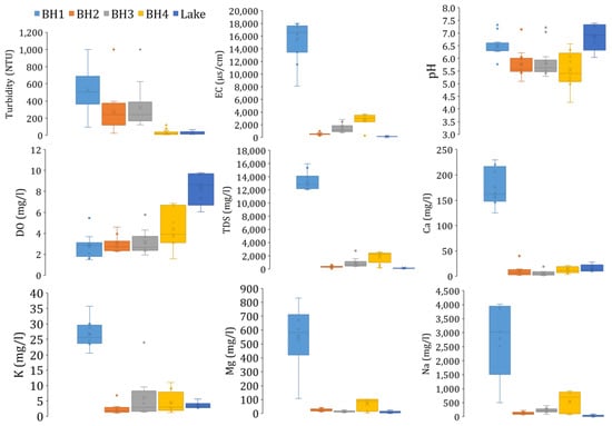
Figure 7.
Boxplots of physico-chemical parameters (Turbidity, EC, pH, DO and TDS) and ion concentrations (Ca, Mg, Na, K). Boxes represent the central half of the data, with the bar in the middle as the median; start of bottom whisker and end of the top whisker represents the lowest and highest values that are not outliers; circles are outliers outside 10th and 90th percentiles.
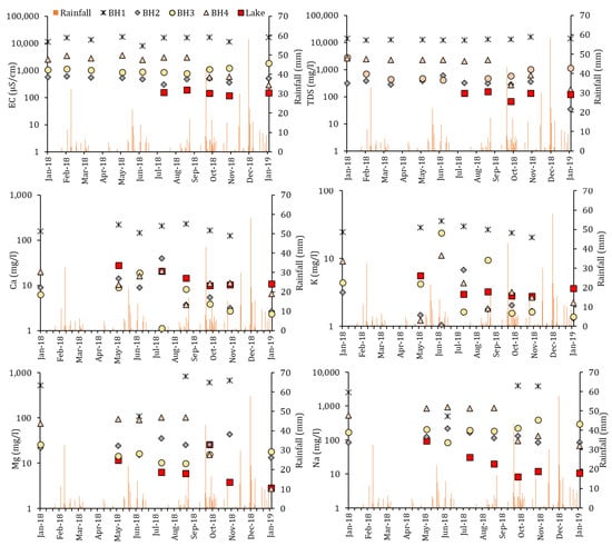
Figure 8.
Temporal variation of the physico-chemical parameters and rainfall in the groundwater and the lake water collected from the study area.
Another important observation that can be made from Figure 8 is that during the rainy periods (September–November 2018) sodium and magnesium concentrations in BH1 groundwater increased. This may indicate some hydrogeological processes that are taking place near BH1 during rainy periods.
3.6. Variation of Groundwater Quality and Its Suitability as Drinking Water Supply
The pH value of samples in BH1, BH2, BH3 and BH4 were in the ranges 5.8–7.3, 5.1–7.1, 5.3–7.2 and 4.3–6.6, respectively (Figure 7). The average pH values of analysed groundwater samples of BH1, BH2, BH3 and BH4 were below the recommended minimum acidic value of 6.5 by WHO [50] and ADWG [51]. Both BH2 and BH4 had about 92% of the samples below the minimum safe prescribed limit for drinking water, followed by BH3 with about 85%, while BH1 was 62%. In general, the groundwater of the study area could be described as slightly acidic. The acidic nature of water could be as a result of the high mineral rich rocks making up the aquifers. The minimum and maximum values of turbidity obtained in all the four monitoring boreholes exceeded the recommended limit of 5 NTU by World Health Organisation (WHO) and Australian Drinking Water Guidelines (ADWG). BH1 groundwater is the most turbid, followed by BH3 and BH4, respectively. High levels of turbidity are an indication of possible presence of contaminants. If the groundwater is to be used directly for drinking, it shows all four are unsuitable as they exceeded the turbidity limit of 5 NTU limit [50,51].
The minimum value of EC in BH1 groundwater, as given in Table 4, exceeded both the minimum and maximum values of EC in BH2, BH3 and BH4, as shown in Figure 7 and Figure 8. The average EC of BH1 groundwater was 15,530 µS/cm. BH2 with average EC of 550 µS/cm was the least. Using the average EC values to classify the boreholes, BH1 is highly saline, BH3 and BH4 are moderately saline, whereas BH2 is slightly saline [52]. Higher EC in the groundwater of BH1 indicates that there could be some localised sources of contamination that has resulted in higher EC levels such as fluid migration into the aquifer from nearby formations. Additionally, it can be due to saltwater intrusion as it is close to an estuary (about 10 km). The high salinity in the groundwater in the Wianamatta Group of formation is due to the high proportion of soluble salts of marine origin available for dissolution, leaching and mobilisation [39]. Moreover, significant increase in concentration of dissolved solids and the presence of metallic ions may be responsible for high EC [53]. Enrichment of salt because of evaporation effect and leaching also cause high level of EC in groundwater [54]. When a source of drinking water becomes more saline, it is expensive to provide potable water both in terms of capital and operating costs.
The TDS concentrations of BH1, BH2, BH3 and BH4 were in the ranges 12,082–15,974 mg/L, 277–613 mg/L, 419–1550 mg/L and 2042–2590 mg/L, respectively. The WHO recommends TDS concentration of 600–1000 mg/L for drinking water purposes; the minimum TDS value of BH2 and BH3 were below WHO guidelines, while only the maximum TDS value of BH2 was meeting the guideline value. In addition, 82% of BH2 groundwater samples analysed were below the minimum 600 mg/L guideline value, while the remaining 18% were within the 600–1000 mg/L WHO threshold limit. A total of 50% of BH3 groundwater samples analysed were the minimum 600 mg/L, 30% was above the maximum 1000 mg/L prescribed limit, while 20% was within the recommended WHO range. Both BH1 and BH4 recorded 100% of samples that were above the maximum 1000 mg/L limit. Therefore, the groundwater collected from BH1 and BH4 are unfit for drinking without adequate treatment. BH1 samples exhibited a higher standard deviation, which suggests local variation in point sources, soil type, and multiple aquifer system [54].
The abundance in cation ranges from Na followed by Mg, Ca and K, respectively. The concentrations of these cations in groundwater are usually greater than 1 mg/L [55,56]. The Na concentration of BH1 groundwater ranged from 3034 to 4047 mg/L, with an average value of 3654 mg/L, BH2 varied between 66 to 202 mg/L, with an average of 138 mg/L, BH3 was within 15 to 304 mg/L, with an average of 214 mg/L, while BH4 ranged from 15 to 107 mg/L, with an average value of 85 mg/L, respectively. Some of the possible reasons for the high Na observed in BH1 compared to others could be due to the saltwater intrusion or some local source. Saltwater intrusion could be a likely cause as the nearest estuary is about 10 km from the catchment area. However, this needs to be further investigated. According to WHO standard, the maximum permissible limit (MPL) for Na is 200 mg/L [50] and BH1 minimum and maximum values exceeded this value. Groundwater samples collected from BH2 and BH4 met WHO Na concentration requirement for drinking purposes whereas 60% of analysed groundwater samples from BH3 exceeded it.
The second dominant cation is Mg and WHO prescribed limit for Mg in drinking water is 100–300 mg/L. The Mg concentration of the samples analysed from BH1 ranged from 562 to 840 mg/L, BH2 ranged from 11 to 40, BH3 ranged from 13.18 to 20.45 and BH4 was 95.3 to 106.7 mg/L. As per WHO minimum prescribed limit of 100 mg/L for Mg concentration in drinking water, both BH2 and BH3 were below the limit. On the contrary, BH1 exceeded both the minimum and maximum permissible limit (100–300 mg/L). About 50% of the samples collected from BH4 were below the minimum permissible limit while the remaining 50% were within the WHO range of 100–300 mg/L [50]. The WHO guideline value for Ca concentration in drinking water is 100–300 mg/L. The groundwater samples collected from BH1 did not exceed the maximum limit. For the rest of the boreholes, Ca concentrations were below the minimum permissible limit, which is 100 mg/l. Both Mg and Ca ions contribute to water hardness but do not pose any health threat [50].
Season has an influence on groundwater quality variability with respect to iron. The concentration of iron in groundwater during rainy season is higher than during dry season. This could be attributed to influence of rainfall infiltrating and dissolving mineral in rocks and soil which are leached into groundwater sources [56]. The average values and standard deviation values of iron for each borehole are presented in Table 4. The ADWG and WHO recommended guideline value of iron for drinking water purposes is 0.3 mg/L. However, all four boreholes exceeded iron guideline value. The metabolic activity of bacteria impacts on the concentration of iron found in groundwater. Iron concentrations above the 0.3 mg/L value may produce bad odour, colour, scaling and corrosion. High iron concentrations are commonly found in shallow wells of less than 30 m deep than in deeper wells [51,57]. Water that contains iron does not have any harmful effect when consumed by human beings. Long term consumption of drinking water with high iron concentration could cause liver disease. Communities can reject groundwater as a source of water supply when the water is coloured due to high iron concentration [56].
3.7. Groundwater Quality for Use as Irrigation Water
Irrespective of the sources of irrigation waters, they still carry certain chemical substances in solution, dissolved from the rocks or soils over which the waters have passed. The quality of irrigation water for use is determined by the concentration and nature of these dissolved constituents [57]. The suitability of groundwater for irrigation purposes is directly linked to the effect of mineral constituents of water on plants and soil. The irrigation quality of groundwater is assessed by the total salt concentration, which is measured by electrical conductivity (EC), sodium percentage (% Na), residual sodium carbonate (RSC), permeability index (PI), sodium adsorption ration (SAR) [58,59] and Kelly’s ratio (KR) [60,61]. Irrigation waters are classified based on the concentration of substances in it. EC is a good indicator of the salinity hazard used in classifying water for irrigation use [58]. However, in this study, SAR and % Na which are widely used were adopted to assess the suitability of Wattle Grove groundwater for irrigation purposes.
The Wilcox diagram [58] was used to evaluate the boreholes water suitability for irrigation purposes (Figure 9a). The SAR values obtained from the boreholes were analysed in accordance with US Salinity Laboratory diagram (USSL) [45] (Figure 9b). As per USSL classification, BH1 groundwater is not suitable for irrigation (Figure 9a). This classification is also reflected in Wilcox diagram (Figure 9b). The groundwater collected from BH1 is classified as C4–S3, indicating extremely high conductivity and salinity (Figure 9b). C4 is not recommended for irrigation under ordinary conditions but can be used sparingly under very special circumstances [58]. Prolonged use of saline water for irrigation can lead to saline soils [62].
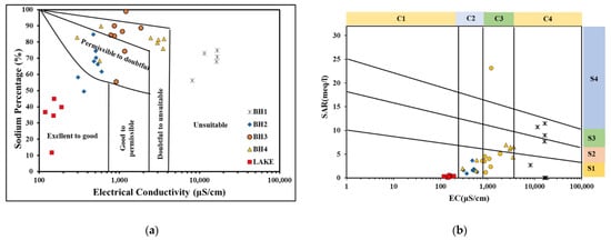
Figure 9.
(a) Suitability of groundwater for irrigation in the Wilcox [58] diagram, (b) US Salinity Laboratory (USSL) [45] diagram for the four boreholes. Note: S1, S2, S3 and S4 represent low, medium, high and very high sodium hazard, respectively, whereas C1, C2, C3 and C4 represents low, medium, high and very high salinity hazard, respectively.
In the case of BH2, about 93% (Table 5) of the samples fell under C2–S1, and the rest as C1–S1 (Figure 9b). C2 can be used when a moderate amount of leaching occurs. However, since the groundwater is of low salinity (S1), it can be used to irrigate many soils without causing developmental issues associated with high level sodium concentration. This is also reflected in the Wilcox diagram (Figure 9a), whereby approximately 80% of the samples collected from BH2 were found in the class of permissible to doubtful, whereas 20% of the samples were in the class of excellent to good for irrigation.
Table 5.
Classification of groundwater samples collected from the four monitoring boreholes for irrigation purposes on the basis of EC, SAR and %Na.
SAR of BH3 groundwater revealed medium, high and very high values, whereas the EC appears to be relatively stable under C3 (Figure 9b). Generally, BH3 groundwater can be used to irrigate plants with moderate salt tolerance under very special conditions. As per USSL classification, about 73% (Table 5) of the groundwater samples of BH3 were in the class of doubtful to unsuitable, while the rest were permissible to doubtful for irrigation purposes. These results indicate that the groundwater may not be suitable for irrigation. If used, it should accompany salinisation mitigation plan.
Finally, suitability of BH4 groundwater is classified as C2/C3–S1/S2. The value of S2 can present sodium hazard in fine-textured soils of high cation-exchange capacity under low-leaching conditions but may be used on coarse-textured soils that have good permeability. The implication of its very high conductivity and medium salinity is that it can be used to irrigate plants on coarse-textured soils but under very special circumstances [61]. In the case of BH4 groundwater samples about 80% fell in doubtful to unsuitable category for irrigation purposes and the remainder were in the class of permissible to doubtful (Figure 9a, Table 5).
The above results indicate that the groundwater is generally unsuitable for irrigation without appropriate treatment. However, the lake water appears to be excellent for irrigation as per both USSL and Wilcox classifications (Figure 9).
3.8. Hydrogeochemical Analysis
Gibbs plots indicate the evaporation dominance in BH1 and few BH4 groundwater samples, whereas BH2, BH3 and some BH4 groundwater samples shows dominance of rock-water interaction (Figure 10a). The average (Ca2+ + Mg2+)/TZ+ ratio (where TZ+ is total cations) at BH2, BH3 and BH4 was 0.2, indicating high abundance of sodium and potassium ions and it justifies the silicate weathering in the study area, whereas average (Ca2+ + Mg2+)/TZ+ ratio for BH1 was 0.5 indicating a stable hydrogeochemical weathering (Figure 10b) [8]. It may be noticed from the plot of calcium and magnesium versus total cations (Figure 10b) that the data points lie below the 1:1 line and it is more prominent at higher TZ+ concentrations. Similarly, at higher cation concentrations, (Na+ + K+) concentration appears to dominate cations (Figure 10c). This is characteristic of the Wianamatta group [39]. Moreover, Mg2+/Na+ vs. Ca2+/Na+ bivariate plots show that groundwater clusters are within the range of global average silicate and evaporites zone (Figure 10d). Therefore, from the above geochemical data, it can be concluded that the dissolution/weathering of silicate rock acts as a major contributor for Na and K ions in BH2, BH3 and BH4, whereas evaporites are responsible for the enriched dissolved solids in the groundwater of BH1.
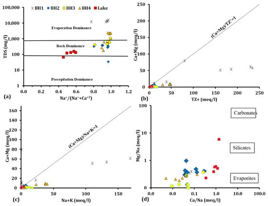
Figure 10.
(a) Gibbs’ diagram representing the ratio of (Na+)/(Na+ + Ca2+) as a function of TDS, (b) (Ca2+ Mg2+) vs. TZ+, (c) (Ca2+ + Mg2+) vs. (Na+ + K+), (d) (Mg2+ /Na+) vs. (Ca2+ /Na+).
3.9. Correlation Analysis
The physico-chemical parameters and water table elevations were analysed using the SPSS Statistical software to calculate Pearson’s correlation coefficient (r). This analysis was carried out for each of the boreholes as well as for the combined data. The study indicated that the correlation analysis for individual boreholes did not show any specific discernible interactions. However, the combined correlation analysis appears to indicate significant correlation between EC, TDS, Turbidity and pH (Table 6). There is a significant positive (green box in Table 6) correlation between turbidity and TDS. The turbidity of the groundwater was observed to be significantly high, which is in the range of 33 to 530 NTU. This means that the turbidity may be caused by the colloidal particles generated by the salt precipitate.
Table 6.
Correlation matrix for physicochemical parameters for all boreholes.
Sodium is found to be having positive correlation with dissolved oxygen (DO). This means that when the DO is higher, there is increased sodium concentration. Higher DO occurs due to increased recharge during the rainfall events. This can be related to the possibility of sodium leaching into the groundwater when recharge occurs. This may be due to the rise in the groundwater table, which may be helping the dissolution of the sodium-based salts present in the soil. Additionally, it can be noted that there is a significant positive correlation between pH, Mg, K and Ca.
4. Conclusions
The aim of this study was to estimate the groundwater recharge for an urban catchment and to assess the groundwater quality. This was achieved by monitoring four boreholes installed in the selected urban area of Wattle Grove, which is located in inner Sydney of New South Wales, Australia. The methodology proposed for urban groundwater recharge estimation is a modified water table fluctuation (WTF) method that used the average specific yield in the WTF equation to account for specific yield variation with respect to geology and depth. Additionally, the methodology included estimation of lateral flows using no or low rainfall conditions and then use this data to estimate the recharge during high rainfall conditions. The results indicate that the method can be used under significantly varying water table depths.
The study shows that the daily groundwater recharge for the study varied between 1.37 to 5.23 mm/day during the days of high rainfall. Not all amount of rainfall contributes to recharge due to the canopy interception, the amount of storage available above and below ground and specific yield. The variation of recharge estimates across the four sites within the study area could be attributed to different surface topography, presence of water bodies and underground water movement.
Recharge values for BH3 and BH4 indicate about 2 to 5 mm/day due to the presence of the lake in the area. This means that it may be possible to achieve an increased groundwater recharge due to the lake and this can help in controlling stormwater flows in urban areas. Water quality of all boreholes met the guidelines of Australian Drinking Water Guidelines (ADWG) and World Health Organization (WHO) standards in terms of pH, calcium, and potassium concentrations. The pH values indicate that the groundwater in the area is slightly acidic. The EC values of groundwater varied across the study area. Generally, the ionic dominance for freshwater is in the order of Na > Mg > Ca > K and all four boreholes’ results agreed with it. There was a strong correlation between electrical conductivity (EC), total dissolved solids (TDS), Turbidity and pH.
It is noted that the increase in the recharge resulted in the higher sodium concentration in the groundwater. The turbidity in the groundwater was observed to be high (33 to 530 NTU). It appears that the source for the high turbidity can be due to the colloidal particle generated by the precipitation of the salt. Due to the presence of high turbidity and salt, it was concluded that the groundwater is not suitable for drinking purposes.
Both the USSL and Wilcox diagrams revealed that the suitability of groundwater for irrigation varied across the site, and the groundwater may be used for irrigation only after appropriate treatment.
This study highlights the recharge and water quality issues associated with the coastal towns. As indicated in the discussions, further studies are required to develop a methodology for estimating recharge in the urban areas and the effect that would have on the groundwater quality in terms of controlling saltwater intrusion.
Author Contributions
D.H. conceptualised the study and contributed to the development of the methodology and revision of the manuscript with discussions. S.N.E. collected and presented the data and prepared the first draft. N.P. helped in the analysis of the data and included relevant literature in the analysis. M.M.R. carried out statistical analysis of the data and contributed to the discussion. B.M. and Z.S. proofread the manuscript and contributed to discussions. All authors have read and agreed to the published version of the manuscript.
Funding
We acknowledge Liverpool City Council (LCC) for partial funding of this project.
Data Availability Statement
Not applicable.
Acknowledgments
We express our gratitude to staff of LCC namely Maruf Hossain, Madhu Pudasaini, Joel Daniels and Sai Natarajan for their support and encouragement. Additionally, sincere thanks to laboratory staff at the Environmental Engineering lab of School of Computing, Engineering and Mathematics (SCEM)–Kiran KC, Upul Jayamaha and Tosin Famakinwa for their help in lab and field work. Finally, huge thanks to colleagues at SCEM lab, namely, Alireza Aghajani Shahrivar and Woo Taek Hong for their help.
Conflicts of Interest
The authors declare no conflict of interest. The funders had no role in the design of the study, in the collection, analyses, or interpretation of data, in the writing of the manuscript, or in the decision to publish the results.
References
- Gatto, E.; Lanzafame, M. Water resource as a factor of production-water use and economic growth. In Proceedings of the 5th ERSA Conference, Amsterdam, The Netherlands, 23–27 August 2005. [Google Scholar]
- Lerner, D.N.; Harris, B. The relationship between land use and groundwater resources and quality. Land Use Policy 2009, 26, S265–S273. [Google Scholar] [CrossRef]
- Chinnasamy, P.; Maheshwari, B.; Dillon, P.; Purohit, R.; Dashora, Y.; Soni, P.; Dashora, R. Estimation of specific yield using water table fluctuations and cropped area in a hardrock aquifer system of Rajasthan, India. Agric. Water Manag. 2018, 202, 146–155. [Google Scholar] [CrossRef]
- Garcia-Fresca, B.; Sharp, J.M. Hydrogeologic considerations of urban development: Urban-induced recharge. Rev. Eng. Geol. 2005, 16, 123–136. [Google Scholar]
- Tubau, I.; Vázquez-Suñé, E.; Carrera, J.; Valhondo, C.; Criollo, R. Quantification of groundwater recharge in urban environments. Sci. Total Environ. 2017, 592, 391–402. [Google Scholar] [CrossRef]
- Thomas, A.; Tellam, J. Modelling of recharge and pollutant fluxes to urban groundwaters. Sci. Total Environ. 2006, 360, 158–179. [Google Scholar] [CrossRef] [PubMed]
- Appleyard, S. The impact of urban development on recharge and groundwater quality in a coastal aquifer near Perth, Western Australia. Hydrogeol. J. 1995, 3, 65–75. [Google Scholar] [CrossRef]
- Pant, N.; Rai, S.P.; Singh, R.; Kumar, S.; Saini, R.K.; Purushothaman, P.; Nijesh, P.; Rawat, Y.S.; Sharma, M.; Pratap, K. Impact of geology and anthropogenic activities over the water quality with emphasis on fluoride in water scarce Lalitpur district of Bundelkhand region, India. Chemosphere 2021, 279, 130496. [Google Scholar] [CrossRef] [PubMed]
- Wu, X.; Zhang, W.; Du, S.; Shi, X.F.; Yu, X.; Huan, Y.; Wang, H.; Jiao, X. Migration and transformation of manganese during the artificial recharging of a deep confined aquifer. Arab. J. Geosci. 2016, 9, 1–12. [Google Scholar] [CrossRef]
- Pant, N.; Dubey, R.K.; Bhatt, A.; Rai, S.P.; Semwal, P.; Mishra, S. Soil erosion and flood hazard zonation using morphometric and morphotectonic parameters in Upper Alaknanda river basin. Nat. Hazards 2020, 103, 3269–3301. [Google Scholar] [CrossRef]
- Smith, M.; Cross, K.; Paden, M.; Laban, P. Spring—Managing Groundwater Sustainably; IUCN: Gland, Switzerland, 2016.
- Groundwater Monitoring Event; Environmental Strategies Pty Ltd.: Liverpool, Australia, 2015; Available online: https://www.prysmiancable.com.au/wp-content/uploads/2016/03/Groundwater-Monitoring-Liverpool-Jan-2015.pdf (accessed on 28 April 2019).
- Oliveira, P.T.; Leite, M.B.; Mattos, T.; Nearing, M.A.; Scott, R.L.; de Oliveira Xavier, R.; da Silva Matos, D.M.; Wendland, E. Groundwater recharge decrease with increased vegetation density in the Brazilian cerrado. Ecohydrology 2017, 10, e1759. [Google Scholar] [CrossRef]
- Scanlon, B.R.; Reedy, R.C.; Stonestrom, D.A.; Prudic, D.E.; Dennehy, K.F. Impact of land use and land cover change on groundwater recharge and quality in the southwestern US. Glob. Change Biol. 2005, 11, 1577–1593. [Google Scholar] [CrossRef]
- Todd, D.K.; Mays, L.W. Groundwater Hydrology Edition; Wiley: Hoboken, NJ, USA, 2005. [Google Scholar]
- Tompson AF, B.; Carle, S.F.; Rosenberg, N.D.; Maxwell, R.M. Analysis of groundwater migration from artificial recharge in a large urban aquifer: A simulation perspective. Water Resour. Res. 1999, 35, 2981–2998. [Google Scholar] [CrossRef]
- Adelana, M. Understanding of Groundwater Recharge for Sustainable Water Resource Management in Northern Victoria: A Review; Project number 104237; Department of Primary Industries: Melbourne, Australia, 2011.
- Lerner, D.N. Identifying and quantifying urban recharge: A review. Hydrogeol. J. 2002, 10, 143–152. [Google Scholar] [CrossRef]
- Yang, Y.; Lerner, D.; Barrett, M.; Tellam, J. Quantification of groundwater recharge in the city of Nottingham, UK. Environ. Geol. 1999, 38, 183–198. [Google Scholar] [CrossRef]
- Lee, L.J.E.; Lawrence, D.S.L.; Price, M. Analysis of water-level response to rainfall and implications for recharge pathways in the Chalk aquifer, SE England. J. Hydrol. 2006, 330, 604–620. [Google Scholar] [CrossRef]
- Krzeminska, D.; Bogaard, T.; Debieche, T.; Cervi, F.; Marc, V.; Malet, J.P. Field investigation of preferential fissure flow paths with hydrochemical analysis of small-scale sprinkling experiments. Earth Surf. Dyn. 2014, 2, 181–195. [Google Scholar] [CrossRef] [Green Version]
- Healy, R.W.; Cook, P.G. Using groundwater levels to estimate recharge. Hydrogeol. J. 2002, 10, 91–109. [Google Scholar] [CrossRef]
- Crosbie, R.S.; Binning, P.; Kalma, J.D. A time series approach to inferring groundwater recharge using the water table fluctuation method. Water Resour. Res. 2005, 41, 1–9. [Google Scholar] [CrossRef]
- Cai, Z.; Ofterdinger, U. Analysis of groundwater-level response to rainfall and estimation of annual recharge in fractured hard rock aquifers, NW Ireland. J. Hydrol. 2016, 535, 71–84. [Google Scholar] [CrossRef] [Green Version]
- Crosbie, R.S.; Peeters, L.J.; Herron, N.; Mcvicar, T.R.; Herr, A. Estimating groundwater recharge and its associated uncertainty: Use of regression kriging and the chloride mass balance method. J. Hydrol. 2018, 561, 1063–1080. [Google Scholar] [CrossRef]
- Watson, A.; Miller, J.; Fleischer, M.; De Clercq, W. Estimation of groundwater recharge via percolation outputs from a rainfall/runoff model for the Verlorenvlei estuarine system, west coast, South Africa. J. Hydrol. 2018, 558, 238–254. [Google Scholar] [CrossRef] [Green Version]
- Varni, M.; Comas, R.; Weinzettel, P.; Dietrich, S. Application of the water table fluctuation method to characterize groundwater recharge in the Pampa plain, Argentina. Hydrol. Sci. J. 2013, 58, 1445–1455. [Google Scholar] [CrossRef] [Green Version]
- Harrington, N.; Cook, P. Groundwater in Australia; National Centre for Groundwater Research and Training: Bedford Park, SA, Australia, 2014. [Google Scholar]
- Water NSW, Western Sydney Borefields Project: Groundwater and Aquifers. 2019. Available online: Https://www.waternsw.com.au/_data/assets/pdf_file/0005/151277/Factsheet-_Groundwater-and-Aquifers.pdf (accessed on 20 July 2020).
- Sundaram, B.; Feitz, A.; De Caritat, P.; Plazinska, A.; Brodie, R.; Coram, J.; Ransley, T. Groundwater sampling and analysis—A field guide. Geosci. Aust. Rec. 2009, 27, 95. [Google Scholar]
- Wattle Grove, New South Wales. 2022. Available online: https://en.wikipedia.org/wiki/Wattle_Grove,_New_South_Wales (accessed on 10 April 2022).
- BOM Australian Groundwater Insight. Available online: http://www.bom.gov.au/water/groundwater/insight/#/hydrogeology/aquifer/upper (accessed on 29 April 2019).
- Hagare, D.; Natarajan, S.K.; Maheshwari, B.L.; Hessam, I.; Joyia, U.-T.; Rajanayake, M. Stormwater management through urban lakes. World Water Stormwater Manag. 2015, 22–26. [Google Scholar]
- Natarajan, S.K.; Hagare, D.; Maheshwari, B. Understanding socio-economic benefits of stormwater management system through urban lakes in Western Sydney, Australia. Ecohydrol. Hydrobiol. 2018, 18, 412–419. [Google Scholar] [CrossRef]
- Google Maps. Available online: https://www.google.com.au/maps/place/Wattle+Grove+NSW+2173/@-33.9533842,150.9387474,15.25z/data=!4m5!3m4!1s0x6b129573ed5b3db7:0x5017d681632cef0!8m2!3d-33.9492164!4d150.9424079?hl=en-GB (accessed on 5 June 2022).
- Branagan, D.F.; Packham, G.H. Geology of New South Wales, 3rd ed.; Department of Mineral Resources: Sydney, Australia, 2000; p. 418.
- Downes, P.M.; Pogson, D.J.; Nix, L.; Robson, D.; Sherwin, L. World-Class Mineral Deposits of the Lachlan Orogen, New South Wales—Australia; ASEG2004 Excursion Guide, Geological Survey of New South Wales, Report No. 2004/297; ASEG: Sydney, Australia, 2004. [Google Scholar] [CrossRef]
- Brinckerhoff, P. Remediation Action Plan for UPSS Replacement Moorebank Service Station (7-Eleven), Moorebank, NSW. 2014. Available online: https://www.liverpool.nsw.gov.au/trim/documents?Recordnumber=228536.2014 (accessed on 3 November 2016).
- Australian Government. Hydrogeological Characteristics of Geological Formations in the Hunter Subregion. 2015. Available online: https://www.bioregionalassessments.gov.au/assessments/11-context-statement-hunter-subregion/1141-groundwater-systems (accessed on 20 June 2020).
- Commonwealth Department of Transport and Regional Development, Australia. Geology, Soils and Water. 1997. Available online: https://www.westernsydneyairport.gov.au/sites/default/files/Draft_Environmental_Impact_Statement_1997_Second_Sydney_Airport_Proposal_Technical_Paper_7_Geology_Soils_and_Water.pdf (accessed on 5 January 2019).
- Brinckerhoff, P. Phase 1 Environmental Site Assessment Report for Moorebank Intermodal Terminal. 2014. Available online: https://simta.com.au/wordpress/wp-content/uploads/2016/07/054-Technical-Paper-5_-Environmental-Site-Assessment-Part-B.pdf (accessed on 3 November 2016).
- Australian Government. Hydrogeological Characteristics of the Sydney Basin Bioregion. 2018. Available online: https://www.bioregionalassessments.gov.au/assessments/11-context-statement-sydney-basin-bioregion/1141-groundwater-systems (accessed on 26 June 2020).
- Australian Standards. Methods of Testing Soils for Engineering Purposes. Method 3.6.1, Soil Classification Tests: Determination of the Particle Size Distribution of a Soil—Standard Method of Analysis by Sieving/[Prepared by Committee CE-009, Testing of Soils for Engineering Purposes], 2nd ed.; Standards Australia: Sydney, Australia, 2009. [Google Scholar]
- Scanlon, B.R.; Healy, R.W.; Cook, P.G. Choosing appropriate techniques for quantifying groundwater recharge. Hydrogeol. J. 2002, 10, 18–39. [Google Scholar] [CrossRef]
- Song, J.; Chen, X. Variation of specific yield with depth in an alluvial aquifer of the Platte River valley, USA. Int. J. Sediment Res. 2010, 25, 185–193. [Google Scholar] [CrossRef]
- Richards, L.A. Diagnosis and Improvement of Saline and Alkaline Soils; US Department of Agriculture: Washington, WA, USA, 1954; 160p.
- García-Gaines, R.A.; Frankenstein, S. USCS and the USDA Soil Classification System: Development of a Mapping Scheme; US Army Corps of Engineers: Washington, WA, USA, 2015. Available online: https://usace.contentdm.oclc.org/digital/collection/p266001coll1/id/3757/ (accessed on 15 February 2022).
- Zomorodi, K. Quantifying Groundwater Recharge from Detention Basins to Forested Buffers in New Jersey. In Proceedings of the International Congress on Watershed Management for Water Supply Systems, New York, NY, USA, 29 June–2 July 2003; American Water Resources Association: Middleburg, VA, USA, 2003. [Google Scholar]
- Sacks, L.A.; Swancar, A.; Lee, T.M. Estimating Ground-Water Exchange with Lakes Using Water-Budget and ChemicalMass-Balance Approaches for Ten Lakes in Ridge Areas of Polk and Highlands Counties, Florida; Water-Resources Investigations Report 98-4133; US Geological Survey: Reston, VA, USA, 1998. [Google Scholar]
- EMM. 2015–2016 Groundwater and Surface Water Monitoring Report: Camden Gas Project; EMM Consulting: Sydney, Australia, 2016; Available online: https://www.agl.com.au/-/media/aglmedia/documents/about-agl/how-we-source-energy/camden/camden-document-repository/groundwater-monitoring-reports/nov-18/j16141rp1_fy15-16-annual-water-monitoring-report_v02.pdf?la=en&hash=04F2EF8488B225E2C5E7D8E826FECA79 (accessed on 5 January 2019).
- WHO. Guidelines for Drinking-Water Quality, 4th ed.; World Health Organization: Geneva, Switzerland, 2011. [Google Scholar]
- National Health and Medical Research Council (Australia). Australian Drinking Water Guidelines 6: National Water Quality Management Strategy; Commonwealth of Australia: Sydney, Australia, 2011.
- Rhoades, J.D.; Kandiah, A.; Mashili, A.M. The Use of Saline Waters for Crop Production; FAO irrigation and drainage paper 48; FAO: Rome, Italy, 1992; Chapter 2. [Google Scholar]
- Chukwu, O. Analysis of groundwater pollution from abattoir waste in Minna, Nigeria. Res. J. Diary Sci. 2008, 2, 74–77. [Google Scholar]
- Kumar, M.; Kumari, K.; Ramanathan, A.; Saxena, R. A comparative evaluation of groundwater suitability for irrigation and drinking purposes in two intensively cultivated districts of Punjab, India. Environ. Geol. 2007, 53, 553–574. [Google Scholar] [CrossRef]
- Ackah, M.; Agyemang, O.; Anim, A.K.; Osei, J.; Bentil, N.O.; Kpattah, L.; Gyamfi, E.T.; Hanson, J.E. Assessment of groundwater quality for drinking and irrigation: The case study of Teiman-Oyarifa Community, Ga East Municipality, Ghana. Proc. Int. Acad. Ecol. Environ. Sci. 2011, 1, 186. [Google Scholar]
- Idoko, O.M. Seasonal variation in iron in rural groundwater of Benue State, middle belt, Nigeria. Pak. J. Nutr. 2010, 9, 892–895. [Google Scholar] [CrossRef]
- Fisher, R.S.; Davidson, O.B.; Goodman, P.T. Summary and Evaluation of Groundwater Quality in the Upper Cumberland, Lower Cumberland, Green, Tradewater, Tennessee, and Mississippi River Basins; Kentucky Geological Survey; University of Kentucky: Lexington, Kentucky, 2004. [Google Scholar]
- Wilcox, L.V. The Quality of Water for Irrigation Use; US Department of Agricultural Technical Bulletin: Washington, WA, USA, 1948.
- Hassen, I.; Hamzaoui-Azaza, F.; Bouhlila, R. Application of multivariate statistical analysis and hydrochemical and isotopic investigations for evaluation of groundwater quality and its suitability for drinking and agriculture purposes: Case of Oum Ali-Thelepte aquifer, central Tunisia. Environ. Monit. Assess. 2016, 188, 135. [Google Scholar] [CrossRef] [PubMed]
- Kalpana, L.; Elango, L. Assessment of groundwater quality for drinking and irrigation purpose in Pambar River sub-basin, Tamil Nadu. Indian J. Environ. 2013, 33, 1–8. [Google Scholar]
- Gowd, S.S. Assessment of groundwater quality for drinking and irrigation purposes: A case study of Peddavanka watershed, Anantapur District, Andhra Pradesh, India. Environ. Geol. 2005, 48, 702–712. [Google Scholar] [CrossRef]
- Rahman, M.M.; Hagare, D.; Maheshwari, B.; Dillon, P. Impacts of prolonged drought on salt accumulation in the root zone due to recycled water irrigation. J. Water Air Soil Pollut. 2015, 226, 90–108. [Google Scholar] [CrossRef]
Publisher’s Note: MDPI stays neutral with regard to jurisdictional claims in published maps and institutional affiliations. |
© 2022 by the authors. Licensee MDPI, Basel, Switzerland. This article is an open access article distributed under the terms and conditions of the Creative Commons Attribution (CC BY) license (https://creativecommons.org/licenses/by/4.0/).