Energy Efficient Neighbor Discovery Protocol for Wireless Sensor Networks Using Coprime Numbers

Abstract

In a long-term monitoring wireless sensor network (WSN) application, sensors are frequently deployed in a wide and an unattended geographical area to gather useful information for a long period of time. Although energy efficiency is affected by various factors, the wireless communication unit is typically the most energy-intensive component of wireless sensors. To extend the life of wireless sensors, they alternate between sleep and active modes to conserve energy. Thus, to exchange a message with neighboring sensors, both sending and receiving sensors must discover each other and stay awake simultaneously. This paper proposes a new neighbor discovery protocol (NDP) by enhancing U-Connect, a well-known protocol that constructs neighbor discovery schedules using only a single prime number. Although the proposed method shares the same characteristics as U-Connect, it offers greater flexibility than U-Connect in terms of duty cycles and schedule lengths. Our numerical analysis based on a power-latency ($PL$) product shows that the proposed method is more efficient than other NDPs such as Quorum, U-Connect, Disco, and ECNDP.

1. Introduction

A wireless sensor network refers to a technology in which wireless sensor devices form a network and transmit information wirelessly to provide physical or environmental conditions to a remote server [1,2,3]. Wireless sensors are typically deployed in large areas where replacing or recharging batteries is costly, inconvenient, or impractical. For example, sensors can be deployed around a volcano to monitor the signs of a volcanic eruption. In such applications, it is not feasible to collect sensors, replace batteries, and deploy them back to the sensing field [4,5,6,7,8,9,10,11,12,13,14,15,16].

In general, wireless sensors are generally powered by a built-in battery, and energy efficiency is crucial for extending the lifetime of the monitoring system. To minimize the battery consumption, a wireless sensor toggles between sleep (power saving) and wake-up (active mode for wireless communication) modes. The configuration of sensors’ sleep mode and wake-up mode within a bounded time, is called a sensor schedule. In order to communicate with neighboring sensors, both the sender and receiving neighbor must be in a wake-up mode simultaneously [9,10,17,18,19,20,21].

A scheduling method that enables a sensor to identify other sensors within a transmission range is known as a neighbor discovery protocol (NDP). In general, increasing the frequency of an active slot will decrease a communication latency by providing more frequent overlapping active slots between two neighbors. However, the increased active slots will result in higher energy consumption. Therefore, the goal of NDPs is to find a set of discovery schedule that achieves desired energy efficiency while minimizing the neighbor discovery latency between neighboring sensors. An NDP also ensures that any randomly selected pair of wireless sensors will discover each other within a certain period known as the worst-case discovery latency [8,9,10,17].

In this paper, we introduced a new NDP based on U-Connect [10] and compared the proposed approach with several well-known NDPs including, a method that uses an $n\times n$ grid for the construction of discovery schedules (Quorum [18,20]), and approaches using prime numbers for schedule construction (Disco [9], and U-Connect [10]). The analysis results in [10] show that U-Connect outperforms both Quorum and Disco in terms of the comparison metrics called the power-latency ($PL$)-product. U-Connect relies on a single prime number to construct its discovery schedules, which means the length of the discovery schedules it produces is constrained to that chosen prime number. However, the length of discovery schedules in the proposed approach can be a multiple of any prime number, and our method provides greater flexibility than U-Connect in terms of duty cycles and schedule lengths.

The main advantages of our proposed method, ECNDP, can be summarized as follows:

• Energy efficiency: As shown in Theorem 2, the worst-case discovery latency of ECNDP will be bounded by $n·k$ when two neighboring sensors use the same odd number k for constructing their discovery schedule and the number of active slots in the schedule is set to $(k-1)/2+n·k$. ECNDP can adjust the number of active slots—which is closely tied to an NDP’s energy consumption—to further reduce energy usage during the discovery phase.
• Superior performance: The proposed approach is more energy efficient. One key metric for comparing NDP protocols is the $PL$-product, and as shown in Table 1, the proposed method outperforms others in this aspect.
• Greater flexibility: U-Connect generates discovery schedules of length $p^2$ where p is the selected prime. On the other hand, the proposed method can offer greater flexibility because its discovery schedules are constrained to $n·k$, where k is odd number and n is any positive number (See Table 2 and Table 3 for the set of duty cycles that can be constructed using the proposed method).
• In Theorem 3, we used the Chinese Remainder Theorem (CRT) [22] to demonstrate that overlapping active slot is established any two ECNDP discovery schedules when two distinct coprime numbers k and i. U-Connect relies on prime numbers to construct discovery schedules, whereas our proposed method uses coprime numbers. As a result, ECNDP can generate a wider variety of schedules than U-Connect.

This paper is organized as follows: Section 2 reviews related work. In Section 3, we provided background information and introduce our proposed method, ECNDP. Section 4 presents numerical analysis, Section 5 shows experimental results, and Section 6 offers conclusions and discusses future work.

2. Related Works

In this section, we briefly introduce several well-known NDPs based on grid structures or prime numbers.

In Ref. [18], a grid based NDP called Quorum was proposed. Quorum selects a random row and column from an $n\times n$ grid for the position of active slots, while the remaining slots are configured as sleep slots. Quorum guarantees that any two schedules will have at least two overlapping active slots within a cycle length of $n^2$. Although the Quorum technique is relatively simple and flexible, it is known to be inefficient compared to prime-based NDPs.

There are two well-known prime-based NDPs. One is Disco [9] that uses two prime numbers to construct discovery schedules, and the other is U-Connect [10] that uses only one prime number for the schedule construction. In Disco, a sensor node wakes up during slots whose indices are divisible by one of the selected prime numbers p. U-Connect adds a group of consecutive active slots from the slot index zero to the slot index $(p+1)/2$, and adds periodic active slots when the slot indexes are divisible by the selected prime number p.

In Ref. [10], the authors proposed a new comparison metric called the power latency product ($PL$-product) and showed that U-Connect outperformed Quorum and Disco in terms of $PL$-product values. Note that, since the cycle length of U-Connect is fixed at $p^2$, it can support only a limited set of duty cycles (DCs) for WSN applications. To enhance the flexibility of U-Connect, in this study, we proposed a new scheduling method that supports a wider range of duty cycles (DCs).

3. Extend Coprime Based NDP

In this section, we first provide the background knowledge necessary to understand the proposed NDP. Then, we define a coprime-based schedule approach for WSNs, and then demonstrate that a common active slot exists between any two sensors using the discovery schedule generated by the proposed method.

3.1. Background Knowledge

In many wireless sensor applications, each sensor alternates its transmitter between sleep and active modes. Different schedules may exhibit varying ratios of sleep to active slots within a cycle. A duty cycle is defined as the ratio of active slots to the total number of slots in a schedule, expressed as a percentage. The duty cycle D can be expressed mathematically as follows:

$$D={\displaystyle \frac{A}{T}}\times 100$$

(1)

where A is the number of active slots and T is the total number of slots in a cycle.

Definition 1.

Discovery Schedule: Suppose that a wireless sensor node u has a discovery schedule with a length T, we denote a discovery schedule as a sequence $S_u^T=⟨a_0, a_1, a_2, \dots , a_{T-2}, a_{T-1}⟩$ such that for all i in $[0, T-1]$ and $a_i=0$ or 1. In $S_u^T$, the $i^{th}$ binary number represents the $i^{\mathrm{th}}$ discovery slot in the cycle T. When $a_i=1$, the $i^{t}h$ discovery slot is called an active slot where sensor u must stay awake, whereas the sensor turns off its radio during the $i^{\mathrm{th}}$ slot, called a sleep slot, if $a_i=0$.

Figure 1 illustrates an example of a discovery schedule. The cycle length in Figure 1 is 10, with active slots occurring at indices $0, 1, 2,$ and 5, during which the node keeps its radio unit on for the entire duration of each slot. All other slots, indicated by ‘0’, are sleep slots. Since this scheduling pattern repeats, the figure shows the pattern through the end of the second cycle.

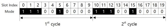
Figure 1. An example schedule of wireless sensor that wake up at slot indexes 0, 1, 2, and 5 within a cycle of length 10.

In WSNs, any randomly selected two sensors within their transmission range are able to communicate with each other. Therefore, any two schedules $S_u^T$ and $S_v^M$ must have at least one common active slot where the neighboring sensors are simultaneously awake. If two schedules have a common active slot, the inner product of two schedule will be greater than or equal to 1, i.e., $S_u^T·S_v^M={\sum }_{i=0}^{L-1}{a}_i·b_i\ge 1$ where $L=LCM(T,M)$, with $LCM$ representing the least common multiple.

During the discovery phase, two neighboring sensors can detect each other only when they are simultaneously active in the same slot. As shown in Figure 2, although the two nodes follow different schedules, they are both active at slot indices 2 and 11, enabling successful discovery.

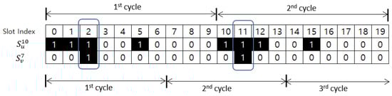
Figure 2. Common active slot: For these two schedules, the common active slots occur at indices 2 and 11.

The Chinese Remainder Theorem (CRT) [22], a fundamental result in number theory, is used to establish the existence of a common active slot in our proposed scheduling method.

Theorem 1.

Let k and n be coprime. Then, the following equations:

$$\begin{array}{cc}& x\equiv a\left(modk\right)\\ \hfill & x\equiv b\left(modn\right)\end{array}$$

(2)

have a unique solution for x mod $kn$.

As an example, for two coprime numbers five and nine, we can find a unique solution for the following modular equations:

$$\begin{array}{cc}& x\equiv 3\left(mod5\right)\\ \hfill & x\equiv 4\left(mod9\right).\end{array}$$

Note that $9\times (-1)+5\times 2=1$. Then, the solution is $x\equiv 9\times (-1)\times 3+5\times 2\times 4=13\left(mod45\right)$. Thus, the solution of the equations above is $13\equiv 58\equiv 103\dots$ and so on.

3.2. Extended Coprime Based Scheduling

In this subsection, we introduce the fundamental properties of the proposed approach, called extended coprime-based neighbor discovery protocol (ECNDP).

Definition 2.

Extended Discovery Schedule: A wireless sensor node u has a discovery schedule $S_u^{n·k}$, where $S_u^{n·k}$ is a binary string of length $n\times k$ for a positive odd number k and a positive number n. $S_u^{n·k}=⟨a_0, a_1, a_2, \dots , a_{(n·k)-2}, a_{(n·k)-1}⟩$ such that $a_i=1$ if $a_i\in \{x|0\le x\le {\displaystyle \frac{k-1}{2}}, k, 2k, \dots , (n-1)k\}$. Otherwise $a_i=0$, where 0 represents a sleep mode and 1 represents an active mode.

For example, if we choose $k=9$ and $n=3$, then length of the schedule is 27, with active slots at indices $0, 1, 2, 3, 4, 9$, and 18, as shown in Figure 3. The first five consecutive slots are active because $\lceil {\displaystyle \frac{k-1}{2}}\rceil ={\displaystyle \frac{9-1}{2}}=4$, which corresponds to Slot 0 through Slot 4. After these initial k slots, any slot whose index is a multiple of 9 becomes an active slot Figure 3. The first five consecutive slots are active because $\lceil {\displaystyle \frac{k-1}{2}}\rceil ={\displaystyle \frac{9-1}{2}}=4$, which corresponds to Slot 0 through Slot 4. After these initial k slots, any slot whose index is a multiple of 9 becomes an active slot.

Figure 3. An example of the proposed scheduling method ECNDP for $k=9$ and $n=3$.

Sensors deployed in a field may not start operating simultaneously, which can lead to asynchronous scheduling among them. To address this issue of slot drifting, the discovery schedule $S_u^{nk}$ is generalized as follows. For an integer $d>0$,

$$S_u^{n·k-1}+d={⟨b_i⟩}_{i=d}^{n·k-1+d}\mathrm{such}\mathrm{that}{b}_{i-d}=a_i.$$

(3)

The proposed approach guarantees the existence of at least one common active slot between any pair of sensors within the cycle length. This claim is supported by Theorems 2 and 3. Theorem 2 addresses the scenario where two sensors use the same discovery schedule generated with a common positive odd integer k. Theorem 3 examines the case where two sensors employ different discovery schedules, generated with coprme positive odd integers k and i, for neighbor discovery.

To demonstrate the existence of a common active slot in the presence of clock drift, we introduce new notation and present the following lemma. For a set $A=\{n_1, n_2, \dots , n_r\}$ and positive integers d and L, we define $A+d=\{(n_i+d)modL:n_i\in A\}.$

Lemma 1.

Let $A=\{n_1,n_2,\dots ,n_r\}$ be a subset of ${\mathbb{Z}}^{+}$. If for some integer $0\le d<L$ there exist $a_i,a_j\in A$ such that

$$d\equiv a_i-a_j(modL),$$

(4)

then $A\cap (A+d)\ne Ø$.

Proof. 

The congruence equation $d\equiv a_i-a_j(modL)$ implies that there exists an integer r such that $a_i-a_j=d+r·L,$ which is equivalent to $a_i\equiv a_j+d(modL).$ Since we defined $A+d=\left\{\right(a+d)modL:a\in A\},$ it follows that the residue class of $a_j+d$ modulo L is an element of $A+d$. But the above congruence shows that this residue class coincides with the residue class of $a_i$, which is an element of A. Therefore, the same residue class lies in both A and $A+d$, implying $A\cap (A+d)\ne Ø.$ □

The following theorem shows that, for any pair of discovery schedules generated with a common odd number, there always exists at least one common active slot between them. In other words, two sensors using these discovery schedules will be able to discover each other regardless of any clock drift between them.

Theorem 2.

Let two sensor nodes u and v have discovery schedules $S_u^{n·k}$ and $S_v^{n·k}$ as given in Definition 2, respectively. If the clock drift of u and v are $d_1$ and $d_2$, respectively, then the schedules $S_u^{n·k}+d_1$ and $S_v^{n·k}+d_2$ have at least one common active slot. That is $(S_u^{n·k}+d_1)·(S_v^{n·k}+d_2)\ge 1$.

Proof. 

Without loss of generality, let $d_1=0$ and $d_2=d>0$. By Definition 2, the parameter k is odd, and therefore ${\displaystyle \frac{k-1}{2}}$ is an integer. Let $A_u$ denote the set of slot indices at which node u is in the active mode in its schedule:

$$A_u=\{amodn·k\mid a\in \{0, 1, \dots , \frac{k-1}{2}, k, 2k, \dots , (n-1)k\}\}.$$

(5)

We show that for every drift d in the range $1\le d\le n·k$, there exist $a_i, a_j\in A_u$ such that $d\equiv a_i-a_j(modn·k).$ Once this is established, Lemma 1 guarantees $A_u\cap (A_u+d)\ne Ø,$ and thus the two schedules overlap.

• Case 1: Clock drift d is in $(0, {\displaystyle \frac{k-1}{2}}]$.

The set $A_u$ contains all consecutive integers from 0 to ${\displaystyle \frac{k-1}{2}}$. Therefore, all differences

$$\begin{array}{cc}\hfill & 1=1-0=2-1=\dots ={\displaystyle \frac{k-1}{2}}-{\displaystyle \frac{k-3}{2}},\hfill \\ \hfill & 2=2-0=3-1=\dots ={\displaystyle \frac{k-1}{2}}-{\displaystyle \frac{k-5}{2}},\hfill \\ \hfill & ⋮\hfill \\ \hfill & {\displaystyle \frac{k-3}{2}}={\displaystyle \frac{k-1}{2}}-1, \mathrm{and}\hfill \\ \hfill & {\displaystyle \frac{k-1}{2}}={\displaystyle \frac{k-1}{2}}-0.\hfill \end{array}$$

(6)

Hence for all integers d such that $0<d\le {\displaystyle \frac{k-1}{2}}$, $A_u\cap (A_u+d)\ne Ø$.

Note that, in the expression $1=1-0$, the left-hand side represents the clock drift, whereas the right-hand side denotes the difference between the active-slot indices 0 and 1 in the set $A_u$. Throughout the subsequent expressions, the left-hand side always denotes the clock drift, while the subtraction on the right-hand side represents the difference between two active-slot indices in the set $A_u$.

• Case 2: Clock drift d is in $[{\displaystyle \frac{k+1}{2}}, k]$.

Since $k\in A_u$, subtracting from the consecutive elements $0, 1, \dots , {\displaystyle \frac{k-1}{2}}$ yields

$$\begin{array}{cc}\hfill & {\displaystyle \frac{k+1}{2}}=k-{\displaystyle \frac{k-1}{2}},\hfill \\ \hfill & {\displaystyle \frac{k+3}{2}}=k-{\displaystyle \frac{k-3}{2}},\hfill \\ \hfill & ⋮\hfill \\ \hfill & k-2=k-2,\hfill \\ \hfill & k-1=k-1,\mathrm{and}\hfill \\ \hfill & k=k-0.\hfill \end{array}$$

(7)

Thus, we know that for all d in $[{\displaystyle \frac{k+1}{2}}, k]$, $A_u\cap (A_u+d)\ne Ø$.

• Case 3: Clock drift d is in $[k+1, k+\frac{k-1}{2}]$.

Since the schedule length is $L=n·k$, the indices wrap modulo L. Because $1\in A_u$, we obtain $1\equiv n·k+1(modn·k)$. Subtracting $(n-1)k\in A_u$ gives $k+1=(n·k+1)-(n-1)k$. Likewise, using the consecutive elements $0,1,\dots ,\frac{k-1}{2}$ in $A_u$, we obtain that

$$\begin{array}{cc}\hfill & k+2=(n·k+2)-(n-1)k,\hfill \\ \hfill & k+3=(n·k+3)-(n-1)k,\hfill \\ \hfill & ⋮\hfill \\ \hfill & k+{\displaystyle \frac{k-1}{2}}=(n·k+\frac{k-1}{2})-(n-1)k.\hfill \end{array}$$

(8)

Thus $A_u\cap (A_u+d)\ne Ø$ for all $d\in [k+1,k+\frac{k-1}{2}]$.

• Case 4: Clock drift d is in $[k+\frac{k+1}{2}, 2k]$.

A similar argument applies. Using $2k\in A_u$ and the consecutive elements in the first block, we obtain that

$$\begin{array}{cc}\hfill & k+{\displaystyle \frac{k+1}{2}}=2k-{\displaystyle \frac{k-1}{2}},\hfill \\ \hfill & k+{\displaystyle \frac{k+3}{2}}=2k-{\displaystyle \frac{k-3}{2}},\hfill \\ \hfill & ⋮\hfill \\ \hfill & 2k-1=2k-1,\mathrm{and}\hfill \\ \hfill & 2k=2k-0.\hfill \end{array}$$

(9)

Thus each d in $[k+\frac{k+1}{2}, 2k]$ can be expressed as a difference of elements of $A_u$, so $A_u\cap (A_u+d)\ne Ø$.

The same reasoning repeats across all remaining blocks $[2k, 3k], [3k, 4k], \dots , \left[\right(n-1)k, n·k]$. Therefore, for every drift $1\le d\le n·k$, there exist $a_i,a_j\in A_u$ satisfying $d\equiv a_i-a_j(modn·k).$ By Lemma 1, this implies for all d in $(0,n·k]$, $A_u\cap (A_u+d)\ne Ø.$ Thus, the schedules $S_u^{n·k}$ and $S_v^{n·k}+d$ always share at least one common active slot. □

Theorem 2 guarantees that any two sensors employing the extended discovery schedule defined in Definition 2 can successfully discover each other within a single schedule period, even when their clocks are drifted. In other words, the two sensors can communicate successfully without requiring synchronized start times.

The next theorem is about the discovery schedules generated from coprime integers. Because the proposed scheme is based on coprime numbers, without losing generality, we assume $S_u^{n·k}$ and $S_v^{m·i}$ are constructed using two numbers k and i and their highest common factor (or greatest common divisor) is 1. The cycle lengths of $S_u^{n·k}$ and $S_v^{n·i}$ are $n·k$ and $m·i$, respectively. The following theorem shows that the drifted discovery schedules of $S_u^{n·k}$ and $S_v^{m·i}$, $S_u^{n·k}+d_1$ and $S_v^{m·i}+d_2$, have at least one common active slot.

Theorem 3.

For two sensor nodes u and v using a discovery schedule $S_u^{n·k}+d_1$ and $S_v^{m·i}+d_2$, respectively as defined in Definition 2 where n and m are distinct positive integers, the nodes u and v have at least one common active slot within $k·i$ slot times.

Proof. 

By Definition 2, the active slot indexes of u is $d_1, d_1+1, d_1+2, ..., d_1+(k-1)/2, d_1+k, \dots ,d_1+(n-1)·k, d_1+n·k, \dots$. Also, the active slot indexes of v is d₂,$d_2+1, d_2+2, \dots , d_2+(i-1)/2,d_2+i,\dots , d_2+(m-1)·i, d_2+m·i\dots$. Since the selected two numbers k and i are coprime, by the CRT [22], there exists a unique solution to the following system of equations:

$$\begin{array}{cc}& x\equiv d_1\left(modk\right)\\ \hfill & x\equiv d_2\left(modi\right).\end{array}$$

(10)

The solution x represents the index of the common active slot between u and v. Therefore, two sensor nodes u and v can discover each other using a common active slot indexes at $x\equiv x+k·i\equiv x+2k·i\equiv \dots$. □

The scenario is considered asymmetric when the duty cycles (DCs) of different sensor nodes are different. According to Theorem 3, if the two period values ‘k’ and ‘i’ are coprime, the two schedules will share at least one common active slot within $k\times i$ slots. This result indicates that the proposed ECNDP scheme is applicable even in asymmetric scenarios.

4. Numerical Analysis

In this section, we compared the discovery schedules of Quorum, Disco, and U-Connect with our proposed method ECNDP using a numerical metric called $PL$ (power-latency) product [10]. The average power consumption of a schedule $S_u^T$ is defined by $P={\displaystyle \frac{1}{T}}{\sum }_{i=0}^{T-1}{a}_i$ and L represents the worst-case discovery latency. Thus, the power latency product $\lambda$ is defined as the following: $\lambda =PL={\displaystyle \frac{L}{T}}{\sum }_{i=0}^{T-1}{a}_i$.

The Quorum-based NDP in [18,20] uses a matrix to produce discovery schedules. The entries of the matrix are filled with monotonically increasing numbers from one to $n^2$ from the top left to the bottom right corner. Each sensor randomly picks one column and one row from the matrix, and the selected column and row are used for the location of active slots. Therefore, the total cycle length of the quorum-based NDP is $L=n^2$. $P_Q=(2n-1)/n^2$ and the value of $PL$ is ${\lambda }_Q=2\sqrt{(L-1)}\approx 2\sqrt{L}$.

The U-Connect NDP in [10] uses one prime number p to produce a base schedule and adds additional consecutive active slots from the first slot of the discovery cycle to the ${{\displaystyle \frac{p+1}{2}}}^{\mathrm{th}}$ slot. In other words, U-Connect has a set of ${\displaystyle \frac{p+1}{2}}$ consecutive active slots at the beginning of each cycle (of length $p^2$) in addition to the set of periodic active slots where their indexes are divisible by the selected prime number p. The worst-case latency (L) of U-Connect is equal to $p^2$. Therefore, U-Connect becomes a 1.5-approximation algorithm for neighbor discovery. More precisely, the average energy consumption of U-Connect ($P_U$) is ${\displaystyle \frac{\frac{p+1}{2}+p}{p^2}}{p}^2\approx {\displaystyle \frac{\frac{3}{2}\sqrt{L}}{L}}$. Thus, the $PL$ product of U-Connect is given by ${\lambda }_U={\displaystyle \frac{3p+1}{2}}={\displaystyle \frac{3\sqrt{L}+1}{2}}\approx {\displaystyle \frac{3\sqrt{L}}{2}}$.

Disco in [9] uses two prime numbers for neighbor discovery protocol. The worst case latency is given by $L=p_1{p}_2$, and active slot numbers is givey by $p_1+p_2$. Therefore, the power consumption is ${\displaystyle \frac{p_1+p_2}{p_1{p}_2}}$. The $PL$ product of Disco is ${\lambda }_E=p_1+p_2\ge 2\sqrt{p_1{p}_2}=2\sqrt{L}$.

We give $PL$ product of ECNDP. Since ECNDP uses a single odd number k and a positive integer n. The worst-case latency can be expressed as $L=n·k$. The power consumption of ECNDP is given by ${\displaystyle \frac{1}{L}}({\displaystyle \frac{k-1}{2}}+n)$. Accordingly, the $PL$ product of ECNDP, denoted by ${\lambda }_E$, can be derived as ${\lambda }_E=({\displaystyle \frac{k-1}{2n·k}}+{\displaystyle \frac{1}{k}})n·k={\displaystyle \frac{k-1}{2}}+{\displaystyle \frac{n·k}{k}}\approx {\displaystyle \frac{k}{2}}+{\displaystyle \frac{n·k}{k}}.$ Since k and n are positive integers, by arithmetic–geometric mean inequality, we obtain ${\displaystyle \frac{k}{2}}+{\displaystyle \frac{n·k}{k}}\ge 2\sqrt{{\displaystyle \frac{k}{2}}·{\displaystyle \frac{n·k}{k}}}=2\sqrt{{\displaystyle \frac{n·k}{2}}}=\sqrt{2}\sqrt{L}$. The equality holds if k equals $2n$. Table 1 provides a summary of the $PL$ product for each protocol. The Normalized values express the ratio of each protocol’s $PL$ product relative to the $PL$ products of Quorum and Disco. Since Quorum and Disco both have a normalized value of 1, their $PL$ products are used as the baseline for comparison.

Table 1. $PL$ product of each protocol.

Protocol	Parameters (-)	$\mathit{PL}$ Product (-)	Normalized (-)
Quorum	n	$2\sqrt{L-1}\approx 2\sqrt{L}$	1
Disco	$p_1, p_2$	$2\sqrt{p_1\times p_2}=2\sqrt{L}$	1
U-Connect	p	${\displaystyle \frac{3\sqrt{L}+1}{2}}\approx {\displaystyle \frac{3\sqrt{L}}{2}}$	$0.75$
ECNDP	$k, n$	${\displaystyle \frac{k-1}{2}}+n\approx \sqrt{2}\sqrt{L}$	$0.707$

Table 1. $PL$ product of each protocol.

Protocol	Parameters (-)	$\mathit{PL}$ Product (-)	Normalized (-)
Quorum	n	$2\sqrt{L-1}\approx 2\sqrt{L}$	1
Disco	$p_1, p_2$	$2\sqrt{p_1\times p_2}=2\sqrt{L}$	1
U-Connect	p	${\displaystyle \frac{3\sqrt{L}+1}{2}}\approx {\displaystyle \frac{3\sqrt{L}}{2}}$	$0.75$
ECNDP	$k, n$	${\displaystyle \frac{k-1}{2}}+n\approx \sqrt{2}\sqrt{L}$	$0.707$

Table 2 displays various sets of Duty Cycles (DC) for discovery schedules generated by the proposed method using prime numbers p, with decimal points omitted. The generated schedules have shorter cycle lengths compared to those of U-Connect. Since the DC of ECNDP is ${\displaystyle \frac{\frac{k-1}{2}+n}{nk}}\times 100$, ECNDP can produce more discovery schedules with various DCs than U-Connect. For instance, using odd number three, it is possible to generate nine schedules with DCs of 34%, 35%, 36%, 37%, 38%, 40%, 41%, 44%, and 50%.

Table 2. A set of duty cycles available in ECNDP with various k values.

k (-)	Duty Cycle (%)
3	34, 35, 36, 37, 38, 40, 41, 44, 50
5	21, 22, 23, 24, 25, 26, 28, 30, 33, 40
7	15, 16, 17, 18, 19, 20, 21, 22, 25, 28, 35
11	10, 11, 12, 13, 14, 15, 16, 18, 20, 24, 31
13	9, 10, 11, 12, 13, 14, 15, 16, 19, 23, 30
17	7, 8, 9, 10, 11, 12, 13, 15, 17, 21, 29
19	6, 7, 8, 9, 10, 11, 12, 13, 14, 17, 21, 28
23	5, 6, 7, 8, 9, 10, 11, 12, 13, 16, 20, 28
29	4, 5, 6, 7, 8
31	4, 5, 6, 7, 8
41	3, 4, 5, 6, 7
47	3, 4, 5

Table 2. A set of duty cycles available in ECNDP with various k values.

k (-)	Duty Cycle (%)
3	34, 35, 36, 37, 38, 40, 41, 44, 50
5	21, 22, 23, 24, 25, 26, 28, 30, 33, 40
7	15, 16, 17, 18, 19, 20, 21, 22, 25, 28, 35
11	10, 11, 12, 13, 14, 15, 16, 18, 20, 24, 31
13	9, 10, 11, 12, 13, 14, 15, 16, 19, 23, 30
17	7, 8, 9, 10, 11, 12, 13, 15, 17, 21, 29
19	6, 7, 8, 9, 10, 11, 12, 13, 14, 17, 21, 28
23	5, 6, 7, 8, 9, 10, 11, 12, 13, 16, 20, 28
29	4, 5, 6, 7, 8
31	4, 5, 6, 7, 8
41	3, 4, 5, 6, 7
47	3, 4, 5

Figure 4 provides the pseudocode for determining the parameters of k and n that yield a shorter cycle length and a smaller number of active-mode slots compared to U-Connect. Figure 4 presents an algorithm that explores the search space defined by $k_{val}$, $n<200$ for all feasible pairs $(k_{val},n)$ capable of generating discovery schedules with short cycle length and lower duty cycle.

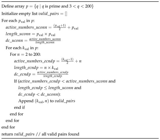
Figure 4. Pseudocode for determining k and n in ECNDP.

Table 3 compares the Duty Cycles (DCs) supported by the proposed method, ECNDP, with those supported by U-Connect. In the first row, U-Connect uses the prime number 13 to generate a schedule with an approximate Duty Cycle (DC) value of 10%. The schedule has 20 active slots, and the length of the schedule is 169. In contrast, the proposed ECNDP offers multiple options to generate a schedule with an approximate DC of 10%. For instance, by using the prime number 13 and setting n to 12, ECNDP produces a cycle of length 156 with 18 active slots. This results in fewer active slots and a shorter cycle length than U-Connect. The 10% row in ECNDP only shows schedules that have shorter cycle lengths and fewer active slots than U-Connect. For DCs in the 1%, 2%, 5%, and 10% ranges, the proposed method demonstrates an ability to generate schedules with fewer active slots and shorter cycle lengths.

Table 3. Comparison of U-Connect and ECNDP in terms of the number of active slots and cycle length at 10%, 5%, 2%, and 1% duty cycles.

U-Connect				ECNDP
DC (%)	$\mathit{p}$ (-)	Num. Active Slots (Slots)	Length (Slots)	DC (%)	$\mathit{k}$ (-)	$\mathit{n}$ (-)	Num. Active Slots (Slots)	Length (Slots)
11.83%	13	20	169	11.53%	13	12	18	156
				11.24%	13	13	19	169
				11.76%	17	8	16	136
				11.11%	17	9	17	153
5.23%	29	44	841	5.11%	29	29	43	841
				5.16%	31	25	40	775
				5.08%	31	26	41	806
				5.02%	31	27	42	837
				5.14%	41	18	38	738
				5.00%	41	19	39	779
				4.87%	41	20	40	820
2.06%	73	110	5329	2.06%	73	71	107	5183
				2.05%	73	72	108	5256
				2.04%	73	73	109	5329
				2.06%	79	62	101	4898
				2.03%	79	64	103	5056
				2.02%	79	65	104	5135
				2.01%	79	66	105	5214
				2.00%	79	67	106	5293
0.99%	151	227	22,801	0.99%	151	150	225	22,650
				0.99%	151	151	226	22,801
				0.99%	157	139	217	21,823
				0.99%	157	140	218	21,980
				0.98%	157	141	219	22,137
				0.98%	157	142	220	22,294
				0.98%	157	143	221	22,451
				0.98%	157	144	222	22,608
				0.97%	157	145	223	22,765

Table 3. Comparison of U-Connect and ECNDP in terms of the number of active slots and cycle length at 10%, 5%, 2%, and 1% duty cycles.

U-Connect				ECNDP
DC (%)	$\mathit{p}$ (-)	Num. Active Slots (Slots)	Length (Slots)	DC (%)	$\mathit{k}$ (-)	$\mathit{n}$ (-)	Num. Active Slots (Slots)	Length (Slots)
11.83%	13	20	169	11.53%	13	12	18	156
				11.24%	13	13	19	169
				11.76%	17	8	16	136
				11.11%	17	9	17	153
5.23%	29	44	841	5.11%	29	29	43	841
				5.16%	31	25	40	775
				5.08%	31	26	41	806
				5.02%	31	27	42	837
				5.14%	41	18	38	738
				5.00%	41	19	39	779
				4.87%	41	20	40	820
2.06%	73	110	5329	2.06%	73	71	107	5183
				2.05%	73	72	108	5256
				2.04%	73	73	109	5329
				2.06%	79	62	101	4898
				2.03%	79	64	103	5056
				2.02%	79	65	104	5135
				2.01%	79	66	105	5214
				2.00%	79	67	106	5293
0.99%	151	227	22,801	0.99%	151	150	225	22,650
				0.99%	151	151	226	22,801
				0.99%	157	139	217	21,823
				0.99%	157	140	218	21,980
				0.98%	157	141	219	22,137
				0.98%	157	142	220	22,294
				0.98%	157	143	221	22,451
				0.98%	157	144	222	22,608
				0.97%	157	145	223	22,765

Table 4 compares the lengths of discovery cycles in ECNDP with those of Disco and U-Connect for the selected Duty Cycles, ranging from 1% to 10%. As shown in Table 4, the cycle length of ECNDP is only 47% of that of Disco and 90% of U-connect on average.

Table 4. Comparison of ECNDP, Disco and U-Connect in terms of the length of discovery schedules.

DC (%)	${\mathit{p}}_1, {\mathit{p}}_2$ (-)	Len. (Slots)	p (-)	Len. (Slots)	$\mathit{k}, \mathit{n}$ (-)	Len. (Slots)	Disco:ECNDP (-)	U-Connect:ECNDP (-)
10%	17, 23	391	13	169	17, 8	136	1:0.35	1:0.80
5%	37, 43	1591	29	841	41, 18	738	1:0.46	1:0.88
2%	93, 103	9579	73	5329	79, 64	5056	1:0.35	1:0.95
1%	197, 199	39,203	151	22,801	157, 139	21,823	1:0.56	1:0.96
Average	-	-	-	-	-	-	1:0.47	1:0.90

5. Experimental Analysis

In this study, we utilized the OMNeT++ 6.0.2 simulator for our performance evaluation, leveraging the INET framework, which includes various wired and wireless components [23]. We randomly deployed 50 sensor nodes for the experiments as shown in Figure 5. For communication, we utilized the IEEE 802.15.4 protocol as the standard, with CSMA/CA-based communication implemented at the MAC layer. The experiments were conducted in a symmetric environment with duty cycles of 10%, 5%, 2%, and 1%. Communication was carried out in a bidirectional, broadcasting manner. The algorithms considered in this study include U-Connect, Quorum, Disco, and the proposed ECNDP.

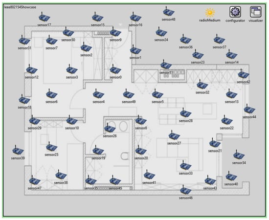
Figure 5. OMNeT++ simulator.

Table 5 and Table 6 present the simulation settings. We conducted 20 random simulation runs for each duty cycle using the parameters p, k, and n shown in Table 7. In the simulation, “Active” refers to the state in which a node is transmitting, receiving or listening. Thus, if a node remains in Active mode continuously, it stays engaged in these operations throughout each slot, leading to significantly higher energy consumption.

Table 5. Power consumption parameters in different modes.

Mode	INET Parameter Name	Default Value
Listening	Receiver Idle Power Consumption	0.005 mW
Receiving	Receiver Receiving Power Consumption	50 mW
Transmitting	Transmitter Transmitting Power Consumption	75 mW

Table 6. Configuration setting of OMNeT++ simulator.

Division	Configuration Setting Value
Topology	Random deployment (indoor environment)
Network size	$50\mathrm{m}\times 50\mathrm{m}$ (indoor floor plan scale)
Transmission range	$10\mathrm{m}\sim 20\mathrm{m}$ (indoor) [24]
Number of nodes	50 nodes
PHY & Radio model	IEEE802154NarrowbandScalarRadio
Center frequency	2450 MHz (2.4 GHz ISM band)
Transmit power	1 mW (0 dBm)
Receiver sensitivity	$-92$ dBm
Path loss model	LogNormalShadowing ($\alpha =3.0$, $\sigma =4$ dB)
Noise floor	$-96$ dBm (IsotropicScalarBackgroundNoise)
MAC Protocol	IEEE 802.15.4 CSMA/CA
Duty cycle (DC)	10%, 5%, 2%, 1%
Simulator	OMNeT++ 6.0.2 + INET Framework
Algorithms evaluated	Disco, Quorum, U-Connect, ECNDP

Table 7. Parameter settings of each protocols for simulation.

Protocol	10% (-)	5% (-)	2% (-)	1% (-)
ECNDP	$k=17$, $n=8$	$k=41$, $n=18$	$k=79$, $n=64$	$k=157$, $n=139$
U-Connect	$p=13$	$p=29$	$p=73$	$p=149$
Disco	$p_1=17$, $p_2=23$	$p_1=37$, $p_2=43$	$p_1=93$, $p_2=103$	$p_1=197$, $p_2=199$
Quorum	$n=19$	$n=39$	$n=99$	$n=199$

In a typical wireless sensor network, sensors are frequently configured with an extremely low duty cycle because the network must operate on battery power for extended periods, often spanning several months to years. Considering this critical requirement, we selected a 1% duty cycle for the experimental setup and simulation focus. Also, this setting was chosen because, as illustrated in Table 4, the performance difference between the proposed ECNDP protocol and other neighbor discovery protocols (NDPs) diminishes as the duty cycle is lowered. By selecting 1%, we tested its performance at the most constrained operational point.

The discovery delays shown in Figure 6 and Figure 7 are based on the worst-case discovery latency. Even if two nodes discover each other quickly, they must remain in discovery mode—continuing mandatory periodic wake-ups—until the full worst-case discovery duration has elapsed. This is because a node cannot independently determine whether all of its neighbors have been discovered. To guarantee complete neighbor discovery, each node must therefore stay in the discovery phase until the end of its designated discovery cycle. As a result, for nodes with low duty cycles, the worst-case discovery latency for low-duty neighbors can become significantly long.

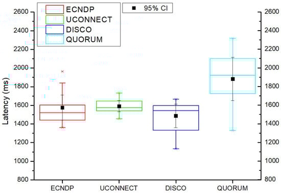
Figure 6. Experimental result of worst-case latency.

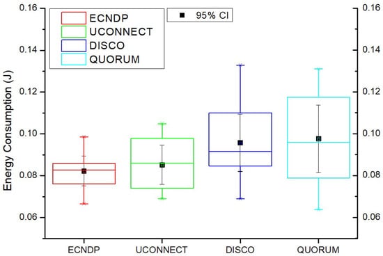
Figure 7. Experimental result of energy consumption.

Figure 6 presents the box plot for simulated cases with 1% duty cycle (DC), illustrating that the proposed method outperforms U-Connect, Disco, and Quorum in terms of latency. The proposed method demonstrates superior overall performance, particularly through its substantially lower standard deviation compared to Disco and Quorum, excluding U-Connect.

In Figure 6, the median latency of ECNDP is approximately 1500 ms, and the narrow interquartile range (IQR) indicates stable performance. Outliers appear near 1850 ms on the upper end, suggesting that under certain conditions the latency can spike, though overall variability remains low. Its median is also lower than that of U-Connect. For U-Connect, the median ranges from 1550 ms to 1600 ms, with an extremely small IQR, reflecting highly stable behavior. There are almost no outliers, and although the average latency is slightly higher, U-Connect exhibits the lowest variability overall. For Disco, the median latency is around 1450 ms —the lowest among the protocols. Its IQR shows a moderate level of dispersion, with almost no outliers. Overall, its variability is higher than ECNDP but more stable than Quorum. For Quorum, the median latency is roughly 1850 ms, the highest among the protocols. Its IQR is also wide, indicating substantial variability and instability. Although it shows no outliers, both the higher latency and the broad distribution reflect less stable performance.

Table 8 presents the mean and variance of the experimental results, while Table 9 shows the results of the ANOVA test. The ANOVA results indicate a statistically significant difference in latency among the four treatments (F(3,36) = 7.83, p <0.001). The treatment effect explains approximately 39.5% of the total variance, indicating a large effect size.

Table 8. Latency experiment summary for each protocol.

Protocol	Num. of Observations (-)	Mean (ms)	Variance (ms2)
ECNDP	10	1514.153	23,817.13216
U-Connect	10	1587.73	6882.080511
DISCO	10	1485.305	31,754.07827
QUORUM	10	1880.178	104,459.8424

Table 9. Analysis of variance (ANOVA) for latency experiment.

Source of Variation	Sum of Squares (ms2)	df (-)	Mean Square (ms2)	F-Value (-)	p-Value (-)	F-Critical (-)
Treatment	980,403.7053	3	326,801.2351	7.8316	0.000377	2.8663
Error	1,502,218.2000	36	41,728.2833
Total	2,482,621.9050	39

ECNDP consistently consumes the least energy with minimal variation, followed by U-Connect. In contrast, Disco and Quorum exhibit significantly higher and more variable energy consumption. These results show that ECNDP provides the most energy-efficient discovery mechanism, while Quorum is the least efficient among the four protocols.

Figure 7 presents the results for energy consumption. ECNDP shows the lowest median energy usage at approximately 0.082J, with a very narrow IQR, indicating stable and consistent performance. A few lower outliers appear, but overall ECNDP demonstrates the best energy efficiency with minimal variability. For U-Connect, the median energy consumption is around 0.085J, slightly higher than ECNDP. Its IQR is moderately sized, suggesting it is less stable, though it exhibits no outliers. Overall, U-Connect performs worse than ECNDP in terms of efficiency and stability.

Disco has a median of about 0.09J, higher than both ECNDP and U-Connect. Its wide IQR indicates substantial variation in energy usage, making its performance less predictable under different conditions. In general, Disco consumes more energy and is less stable.

Quorum shows the highest median energy consumption at approximately 0.095J, along with the widest IQR. Although it has no outliers, the distribution itself is highly variable, resulting in poor efficiency. Overall, Quorum performs worse than all other NDP protocols in terms of energy consumption.

Table 10 and Table 11 summarize the experimental results and the ANOVA analysis for energy consumption. While ECNDP exhibited the lowest mean energy consumption, it showed a higher variance than the other protocols. The results of the ANOVA test reveal that the differences among the protocols are not statistically significant. However, the boxplot in Figure 7 indicates that ECNDP demonstrates superior performance compared to the other protocols. Its IQR is smaller than all other surveyed NPDs, and its median energy consumption is also slightly lower than the others included.

Table 10. Energy consumption experiment summary for each protocol.

Protocol	Num. of Observations (-)	Mean (J)	Variance (${\mathit{J}}^2$)
ECNDP	10	0.082192152	0.000098133
U-Connect	10	0.085189234	0.000170357
DISCO	10	0.095677964	0.000367021
QUORUM	10	0.097628508	0.00050448

Table 11. ANOVA table for energy consumption experiment.

Source of Variation	Sum of Squares (J2)	df (-)	Mean Square (J2)	F-Value (-)	p-Value (-)	F-Critical (-)
Treatment	0.001744	3	0.000581	2.0400	0.1256	2.8663
Error	0.010260	36	0.000285
Total	0.012004	39

6. Discussion and Conclusions

Many studies have investigated energy-efficient design of NDPs in wireless sensor networks including U-Connect, Disco, and Quorum. Among these NDPs, U-Connect outperforms other NDPs according to the $PL$-product metric. However, U-Connect use only one prime number for the construction of discovery schedules, it supports a limited set of duty cycles. This work improves the U-Connect method by introducing a coprime-based NDP. ECNDP always guarantees the existence of a common active slot within a cycle while enhancing energy efficiency. As shown in Table 1, the results of numerical analysis clearly show that ECNDP outperforms U-Connect, Disco, and Quorum in terms of the $PL$-product metric.

The proposed ECNDP uses positive odd numbers, and according to Definition 2, the number of active slots is defined as $(k-1)/2+n·k$, while the cycle length is defined as the product of an odd number k and a positive integer n. Any two ECNDP schedules are always mutually communicable through shared active slots between neighboring sensors. We demonstrate that, in terms of $PL$-products, the proposed method outperforms existing approaches under worst-case scenarios. The key advantage of the proposed approach over existing methods lies in its flexibility in selecting the discovery schedule parameters, k and n. ECNDP allows any odd value for k and any positive value for n enabling the duty cycle length to be tailored to specific application requirements. As shown in Table 4, compared to Disco, the proposed method reduces the length of the discovery cycle by up to 53% for DCs ranging from 10% to 1%. However, the difference between U-Connect and ECNDP is less noticeable, with approximate reductions of 20% for 10% duty cycle, 14% for 5% duty cycle, and 4% for 1% duty cycle. Table 3 provides examples where, for similar Duty Cycles (DCs), the proposed method generates schedules with shorter cycle lengths and greater variety compared to U-Connect.

For the evaluation of the average performance of ECNDP, experiments on latency and energy consumption were conducted using the OMNeT++ simulator. Based on the results, we conclude that the performance of the proposed approach in the average case, is at least comparable to U-Connect and Disco, and clearly outperforms Quorum. Our future work includes implementing and evaluating the proposed method in a real-world testbed environment.

References

- Wei, L.; Chen, Y.; Zhang, Y.; Zhao, L.; Chen, L. PSPL: A generalized model to convert existing neighbor discovery algorithms to highly efficient asymmetric ones for heterogeneous IoT devices. IEEE Internet Things J. 2020, 7, 7207–7219. [Google Scholar] [CrossRef]
- Sun, H.; Meng, Z.; Wang, D.; Li, H. Fedab: A low-latency energy-efficient proactive neighbor discovery protocol in MLDC-WSN. IEEE Access 2023, 11, 22843–22854. [Google Scholar] [CrossRef]
- Shen, Z.; Yang, Q.; Jiang, H. Multichannel neighbor discovery in bluetooth low energy networks: Modeling and performance analysis. IEEE Trans. Mob. Comput. 2023, 22, 2262–2280. [Google Scholar] [CrossRef]
- Han, K.; Luo, J.; Liu, Y.; Vasilakos, A.V. Algorithm design for data communications in duty-cycled wireless sensor networks: A survey. IEEE Commun. Mag. 2013, 51, 107–113. [Google Scholar] [CrossRef]
- Pozza, R.; Nati, M.; Georgoulas, S.; Moessner, K.; Gluhak, A. Neighbor discovery for opportunistic networking in internet of things scenarios: A survey. IEEE Access 2015, 3, 1101–1131. [Google Scholar] [CrossRef]
- Mehmood, G.; Khan, M.S.; Waheed, A.; Zareei, M.; Fayaz, M.; Sadad, T.; Nazri, K.; Azmi, A. An efficient and secure session key management scheme in wireless sensor network. Complexity 2021, 2021, 6577492. [Google Scholar] [CrossRef]
- Huan, X.; He, H.; Wang, T.; Wu, Q.; Hu, H. A timestamp-free time synchronization scheme based on reverse asymmetric framework for practical resource-constrained wireless sensor networks. IEEE Trans. Commun. 2022, 70, 6109–6121. [Google Scholar] [CrossRef]
- Meng, C.; Yan, X.; Guo, L.; Sun, Z.; Wang, P. An energy-efficient asynchronous neighbor discovery algorithm based on cyclic difference set in duty-cycle wireless sensor networks. J. Netw. Comput. Appl. 2024, 226, 103854. [Google Scholar] [CrossRef]
- Dutta, P.; Culler, D. Practical asynchronous neighbor discovery and rendezvous for mobile sensing applications. In Proceedings of the 6th ACM Conference on Embedded Network Sensor Systems, Raleigh, NC, USA, 5–7 November 2008; pp. 71–84. [Google Scholar]
- Kandhalu, A.; Lakshmanan, K.; Rajkumar, R. U-connect: A low-latency energy-efficient asynchronous neighbor discovery protocol. In Proceedings of the 9th ACM/IEEE International Conference on Information Processing in Sensor Networks, Stockholm, Sweden, 12–16 April 2010; pp. 350–361. [Google Scholar]
- Mehmood, G.; Khan, M.Z.; Bashir, A.K.; Al-Otaibi, Y.D.; Khan, S. An efficient QoS-based multi-path routing scheme for smart healthcare monitoring in wireless body area networks. Comput. Electr. Eng. 2023, 109, 108517. [Google Scholar] [CrossRef]
- Khan, S.; Iqbal, W.; Waheed, A.; Mehmood, G.; Khan, S.; Zareei, M.; Biswal, R.R. An efficient and secure revocation-enabled attribute-based access control for eHealth in smart society. Sensors 2022, 22, 336. [Google Scholar] [CrossRef] [PubMed]
- Huan, X.; Chen, W.; Wang, T.; Hu, H. A Microsecond energy-efficient LoRa time synchronization based on low-layer timestamping and asymmetric time translation. IEEE Trans. Veh. Technol. 2024, 73, 7328–7332. [Google Scholar]
- Lee, W.; Youn, J.-H.; Song, T.-S. Asymmetric wake-up scheduling based on block designs for Internet of Things. Ad Hoc Netw. 2024, 162, 103530. [Google Scholar] [CrossRef]
- Chen, W.; Tang; Cui, F.; Chen, C. Research on Energy Harvesting Mechanism and Low Power Technology in Wireless Sensor Network. Sensors 2024, 24, 47. [Google Scholar] [CrossRef] [PubMed]
- Dogra, R.; Rani, S.; Gianini, G. REERP: A Region-Based Energy-Efficient Routing Protocol for IoT Wireless Sensor Networks. Energies 2023, 16, 6248. [Google Scholar] [CrossRef]
- Zheng, R.; Hou, J.C.; Sha, L. Optimal block design for asynchronous wake-up schedules and its applications in multihop wireless networks. IEEE Trans. Mob. Comput. 2006, 5, 1228–1241. [Google Scholar] [CrossRef]
- Jiang, J.; Tseng, Y.-C.; Hsu, C.-S.; Lai, T. Quorum-based asynchronous power-saving protocols for IEEE 802.11 ad hoc networks. Mob. Netw. Appl. 2005, 10, 169–181. [Google Scholar] [CrossRef]
- Shah, S.M.; Sun, Z.; Zaman, K.; Hussain, A.; Ullah, I.; Ghadi, Y.Y.; Khan, M.A.; Nasimov, R. Advancements in Neighboring-Based Energy-Efficient Routing Protocol (NBEER) for Underwater Wireless Sensor Networks. Sensors 2023, 23, 6025. [Google Scholar] [CrossRef] [PubMed]
- Tseng, Y.-C.; Hsu, C.-S.; Hsieh, T.-Y. Power-saving protocols for IEEE 802.11-based multi-hop ad hoc networks. In Proceedings of the Twenty-First Annual Joint Conference of the IEEE Computer and Communications Societies, New York, NY, USA, 23–27 June 2002; pp. 200–209. [Google Scholar]
- Zheng, R.; Hou, J.C.; Sha, L. Asynchronous wakeup for ad hoc networks. In Proceedings of the 4th ACM International Symposium on Mobile Ad Hoc Networking Computing, Annapolis, MD, USA, 1–3 June 2003; pp. 35–45. [Google Scholar]
- Niven, H.L.I.; Zuckerman, H.S. An Introduction to the Theory of Numbers; John Wiley and Sons: Hoboken, NJ, USA, 1991. [Google Scholar]
- OMNeT++ Home Page. Available online: http://www.omnetpp.org (accessed on 10 August 2024).
- Kochhar, A.; Kumar, N. Wireless sensor networks for greenhouses: An end-to-end review. Comput. Electron. Agric. 2019, 163, 104877. [Google Scholar] [CrossRef]
Disclaimer/Publisher’s Note: The statements, opinions and data contained in all publications are solely those of the individual author(s) and contributor(s) and not of MDPI and/or the editor(s). MDPI and/or the editor(s) disclaim responsibility for any injury to people or property resulting from any ideas, methods, instructions or products referred to in the content. |
© 2025 by the authors. Licensee MDPI, Basel, Switzerland. This article is an open access article distributed under the terms and conditions of the Creative Commons Attribution (CC BY) license (https://creativecommons.org/licenses/by/4.0/).