Non-Premixed Filtered Tabulated Chemistry for LES: Evaluation on Sandia Flames D and E

Abstract

The non-premixed filtered tabulated chemistry for large eddy simulations employs numerical filtering to resolve a thin flame front on practical LES numerical grids. The flame structure is modified to be coherent with the domain discretization. The first turbulent combustion application of the non-premixed filtered tabulated chemistry approach is presented. A keen comparison of the flamelet filtering transformation in the premixed and non-premixed regimes is carried out. Three distinctive features are outlined: the flame thickness variation, the filtered manifold transformation, and the model activation dependence on the chosen diffusion flamelet configuration for a non-premixed filtered approach. The model performance is assessed on two real turbulent flame configurations, Sandia flames D and E, employing a three-dimensional tabulation strategy, where the numerical grid is coupled with the model by the third parameter, i.e., the computational cell size. The repercussions of the above cited aspects are carefully assessed. The results demonstrate that the formalism coupling with an SGS modeling function can adequately describe wrinkled flame front effects. The predictions for both the major stable species and the minor ones accurately correspond with the underlying physics. It turns out that there is a substantial variation of the filter effect as a function of the strain rate of the flame and the considered species. The varying filter sensitivity along the manifold influences the response of the model correction terms and the retrieved variables. The non-premixed FTACLES formalism possibilities and conditions for the model’s utilization and optimal performance are clearly stated, to confirm the idea that SGS closure in diffusive combustion can be derived based on filtering arguments, and not only based on statistical approaches.

1. Introduction

Chemistry tabulation is a reduction technique through which the computational time can be significantly reduced while applying complex chemical kinetics [1,2]. This enables the modeling of practically relevant problems, i.e., ethanol spray combustion [3] or oxy-flame combustion [4] with remarkable precision. The flamelet approach is a consolidated chemical database generation methodology [5,6,7], thereupon it has been extended to encompass the solution steadiness [8,9] and dimensionality [10]. On a diffusion flame where the mixing between fuel and oxidizer takes place with sufficiently high gradients, a laminar diffusion flamelet defines the thin layer where combustion occurs plus the surrounding inert mixing region [11,12]. It follows that a set of one-dimensional laminar flamelets can be generated to cover the whole span and thus describe a real laminar flame [13]. The stiff and computationally expensive species transport equations are solved in a pre-processing state, they are parameterized in terms of control variables and stored in a look-up Table [14]. The reason for the outstanding improvement from the computational point of view lies in the fact that the chemical evolution of the system is entirely described by the transport of a few control variables [15].

For diffusion combustion, the classical laminar flamelet approach employs a parameterization in terms of the mixture fraction and the scalar dissipation rate [16], while the Flamelet Progress Variable (FPV) [17,18] adds a reaction progress parameter to the passive scalar. The latter formulation enables the representation of the whole flamelet structure, i.e., the different possible states from the S-shaped curve obtained by analyzing the stoichiometric temperature evolution as a function of the stoichiometric scalar dissipation rate [19]. Presumed probability density functions (PDF) are broadly employed to model the turbulence-chemistry interaction for non-premixed combustion [20,21,22], though other alternatives include conditional source term estimation [23] or artificial inteligence [24]. For premixed combustion, well-known flamelet tabulation methods include the Flamelet Generated Manifold (FGM) [14] and the Flamelet Prolongation of ILDM (FPI) [25]. The typical premixed flame thickness ${\delta }_l^0$ lies in the range [0.1–1] mm [26], and hence cannot be resolved on a large eddy simulation (LES) numerical grid. The Artificially Thickened Flame (ATF) [27] coupled with FGM [28,29,30], and the premixed Filtered Tabulated Chemistry for LES (FTACLES) [31] are two well developed turbulent combustion chemistry tabulation strategies to overcome this difficulty. The modified turbulence chemistry interaction is then carefully addressed employing sophisticated subgrid scale wrinkling models [32,33,34].

The idea of direct flamelet filtering is quite attractive within the Large Eddy Simulation (LES) framework as it directly links the numerical grid resolution and the turbulent combustion model. The premixed FTACLES [31] is a well-known approach whose theoretical foundation is substantiated considering two flame properties: the flame thickness and the laminar flame speed. The former is lower than the grid size, which justifies the use of the filter in order to render it resolvable, while the latter is conserved through the filtering operation if flame wrinkling effects are neglected. Due to intrinsic non-premixed combustion characteristic features, these statements no longer hold for the diffusion controlled regime. It follows that while mathematically alike, a careful theoretical and numerical assessment of the non-premixed FTACLES is highly necessary.

First, a keen comparison of the flamelet filtering transformation in the two regimes is carried out. The main differences are identified, thus the features which could influence the performance, or to which attention should be paid for the non-premixed model application are outlined. The attention is focused on three aspects: the varying flame thickness and the effect over the flame front resolution, the filtered manifold transformation and the retrieved variables description, and the convenience of the chosen diffusion flamelet configuration for a non-premixed filtered approach. The model performance is assessed on real turbulent flame configurations for which numerical studies using flamelet-based tables in both regimes have delivered satisfactory results, thus offering an ideal condition for the formalism comparison. The model response and the influence of the identified characterizing aspects are then carefully assessed.

The main contributions of this paper are two-fold: it presents the first evaluation of the non-premixed FTACLES under turbulent conditions, thus demonstrating the consistency and adequate performance of the formalism. Furthermore, the distinction between premixed and non-premixed flamelet filtering is highlighted, though it was briefly mentioned in previous work [35], where a profound analysis has so far not been carried out. The current study departs from an insightful description of the filtering properties as a function of the combustion regime to theorize on practical implications, and carefully analyze their repercussion on the obtained results. This is quite relevant for the combustion community as it provides a clear perspective of the non-premixed FTACLES formalism possibilities and conditions for the model’s utilization and optimal performance.

The paper is structured as follows: In Section 2, the numerical modeling along with the flamelet filtering concept is introduced. The implementation is described, and the main distinctive features for both the combustion regimes are highlighted. The study cases, Sandia flames D and E are presented altogether with the numerical methods. Section 3 presents the velocity, mixture fraction and temperature profiles, showing that the formalism adequately describes the flow field and the combustion reaction evolution. Subsequently Section 4 digs deeper on the model performance: the species prediction, retrieved from the table is analyzed and the transformation due to the filtering operation is discussed. Hence, this section addresses the effect of the combustion regime employed for the flamelet generation on the chemical flame structure description. Section 5 is devoted to the conclusions and final remarks.

2. Materials and Methods

2.1. Flamelet Equations

In FGM, the flamelet equations [36] are one-dimensional expressions which describe mass, species and energy conservation in a flame-adapted coordinate system

$$\frac{\partial \rho u}{\partial s}+\rho K=0,$$

(1)

$$\frac{\partial \rho u{Y}_i}{\partial s}+\rho K{Y}_i=\frac{1}{L{e}_i}\frac{\partial }{\partial s}\left(\frac{\lambda }{c_p}\frac{\partial Y_i}{\partial s}\right)+{\dot{\omega }}_{Y_i},$$

(2)

$$\frac{\partial \rho uh}{\partial s}+\rho Kh=\frac{\partial }{\partial s}\left[\frac{\lambda }{c_p}\frac{\partial h}{\partial s}+\sum _{1=1}^{N_s}hi\frac{\lambda }{c_p}\left(\frac{1}{L{e}_i}-1\right)\frac{\partial Y_i}{\partial s}\right],$$

(3)

where s is the spatial coordinate perpendicular to the flame front, K the flame stretch rate, $Y_i$ the mass fraction of species i, and h the enthalpy. $L{e}_i$ is the Lewis number of species i, $\lambda$ the thermal conductivity, $c_p$ the specific heat at constant pressure, ${\dot{\omega }}_{Y_i}$ the chemical production rate, and $N_s$ the total number of species.

The counterflow flame configuration can be used to describe diffusion flames, where the two-dimensional flow field effects are taken into account through the local stretch rate K [37]. Thus, a transport equation for the stretch field is solved [38]

$$\frac{\partial \rho uK}{\partial s}=\frac{\partial }{\partial s}\left(\frac{\mu \partial K}{\partial s}\right)-2\rho K^2+{\rho }_2{a}^2,$$

(4)

where a is the applied strain rate $s^{-1}$ and ${\rho }_2$ the density, both at the oxidizer stream. Moreover, the mixture fraction is obtained from the transport of a passive scalar with the assumption of $Le$ equal to unity

$$\frac{\partial \rho uZ}{\partial s}+\rho KZ=\frac{\partial }{\partial s}\left(\frac{\lambda }{c_p}\frac{\partial Z}{\partial s}\right),$$

(5)

The progress variable c is defined as a linear combination of n chemical species

$$c=\sum _{i=1}^n{\gamma }_i{Y}_i,$$

(6)

where ${\gamma }_i$ is a weight factor. For cases where differential diffusion plays a non-negligible role, different approaches can be employed to deal with non-unity $Le$, e.g., through c transport [10], or by means of a generic control variable parameterization [39].

The solution of the flamelet equations at varying K generates a non-premixed low-dimensional manifold, while the equivalence ratio $\theta$ modification is employed for the premixed manifold generation. For an adiabatic condition the thermodynamical and chemical properties $\Phi =\{T,\rho ,\mu ,D,Y_i,{\dot{\omega }}_{Y_i}\}$ can be uniquely parameterized as $\Phi =f(Z,c)$.

2.2. Filtered Reactive Flow Governing Equations

In the tabulated chemistry context, a reactive flow can be described solving the parameterizing variables transport equations together with the continuity and momentum equations. Applying a filtering operation as it would be in LES, for an adiabatic condition, and assuming $Le=1$, the resulting system reads

$$\frac{\partial \overline{\rho }}{\partial t}+\frac{\partial }{\partial x_i}\left(\overline{\rho }{\tilde{u}}_i\right)=0,$$

(7)

$$\frac{\partial \overline{\rho }{\tilde{u}}_j}{\partial t}+\frac{\partial }{\partial x_i}\left(\overline{\rho }{\tilde{u}}_i{\tilde{u}}_j\right)=\frac{\partial }{\partial x_i}{\overline{\tau }}_{ij}-\frac{\partial }{\partial x_i}\overline{{\tau }_{ij}^t}-\frac{\partial }{\partial x_j}\overline{P},$$

(8)

$$\frac{\partial \overline{\rho }\tilde{Z}}{\partial t}+\frac{\partial }{\partial x_i}\left(\overline{\rho }{\tilde{u}}_i\tilde{Z}\right)=\frac{\partial }{\partial x_i}\left(\overline{\rho }\tilde{D}\frac{\partial \tilde{Z}}{\partial x_i}\right)+{\Omega }_Z+{\alpha }_Z,$$

(9)

$$\frac{\partial \overline{\rho }\tilde{c}}{\partial t}+\frac{\partial }{\partial x_i}\left(\overline{\rho }{\tilde{u}}_i\tilde{c}\right)=\frac{\partial }{\partial x_i}\left(\overline{\rho }\tilde{D}\frac{\partial \tilde{c}}{\partial x_i}\right)+{\overline{\dot{\omega }}}_c+{\Omega }_c+{\alpha }_c,$$

(10)

where $\left(\overline{·}\right)$ and $\left(\widetilde{·}\right)$ correspond to the spatial filter and the Favre or mass-weighted spatial filter, respectively. ${\tau }_{ij}$ the shear stress tensor, ${\tau }_{ij}^t$ the SGS stress tensor, and P the pressure. D is the molecular diffusivity, ${\overline{\dot{\omega }}}_c$ the unresolved chemical production term, and employing $\phi$ for the parameterizing variables Z and c, ${\Omega }_{\phi }$ and ${\alpha }_{\phi }$ express the unresolved convective and diffusive contributions

$${\Omega }_{\phi }=-\frac{\partial }{\partial x_i}(\overline{\rho u_i\phi }-\overline{\rho }{\tilde{u}}_i\tilde{\phi }),$$

(11)

$${\alpha }_{\phi }=\frac{\partial }{\partial x_i}\left(\overline{\rho D\frac{\partial \phi }{\partial x_i}}\right)-\frac{\partial }{\partial x_i}\left(\overline{\rho }\tilde{D}\frac{\partial \tilde{\phi }}{\partial x_i}\right),$$

(12)

whose computation will be presented subsequently.

2.3. Filtered Tabulated Chemistry Closure

The FTACLES formalism is based on the idea that if there is no SGS wrinkling, Equations (11) and (12), as well as the unresolved chemical production can be estimated by directly filtering the one-dimensional flamelet solutions. Despite the general validity of the proposed methodology, the flame structure transformation will incontestably change as a function of the chosen configuration. The premixed FTACLES has been derived considering that the mixture fraction does not change along the flamelet, hence the filtering correction terms exclusively attain c equation. Contrarily, regarding the non-premixed FTACLES the flame structure, i.e., Z profile is modified by the filtering operation. Thus, additionally to c equation correction, closure terms are explicitly computed and included in the form of a source term in Z transport equation as well. This section describes the formulation and computation of the closure terms for premixed and non-premixed flamelets. Subsequently, the main differences between the two regimes are briefly exposed.

2.3.1. Premixed Regime

The premixed FTACLES [31] is a strategy in which directly filtering one-dimensional flamelets and carefully addressing the closure terms, both the speed of flame propagation in addition to the filtered flame structure can be correctly retrieved on an LES approach. The model has been combined with dynamic wrinkling procedures [34], and employed on stratified flames with [40,41] and without adiabatic effects [42] as well as on ignition process assessment [43].

The formalism is based on the fact that if there is no wrinkling at the subgrid scale, the propagation speed of the filtered flame front $s_{\Delta }$ does not differ from the laminar flame speed $s_l^0$

$${\rho }_0{s}_{\Delta }={\int }_{-\infty }^{\infty }\overline{\rho }{\tilde{\dot{\omega }}}_c\left(x\right)dx={\int }_{-\infty }^{\infty }\rho {\dot{\omega }}_c\left(x\right)dx={\rho }_0{s}_l^0.$$

(13)

A Gaussian filter, corresponding to the Gaussian distribution with mean zero and variance ${\sigma }^2=\frac{1}{12}{\Delta }^2$ [44], is then employed

$$F\left(x\right)={\frac{6}{\pi {\Delta }^2}}^{1/2}exp\left(-\frac{6x^2}{{\Delta }^2}\right).$$

(14)

where $\Delta$ is the filter size. The model estimates ${\tilde{\dot{\omega }}}_c$ through direct filtering as:

$${\tilde{\dot{\omega }}}_c=\frac{1}{\overline{\rho }}{\int }_{-\infty }^{\infty }\rho \left(x^{\prime }\right){\dot{\omega }}_c\left(x^{\prime }\right)F(x-x^{\prime })d{x}^{\prime }.$$

(15)

Due to the properties of the filter function $F\left(x\right)$, i.e., ${\int }_{-\infty }^{\infty }F\left(x\right)dx=1$, Equation (13) holds and in this way the adequate values for $s_l^0$ are obtained independent of the filter size employed.

The unclosed convective and diffusive terms in Equation (10) are explicitly computed taking into account the filter effect over the flame structure as:

$${\Omega }_c=-\frac{\partial }{\partial x_i}(\overline{\rho u_{i}c}-\overline{\rho }{\tilde{u}}_i\tilde{c})=-{\rho }_0{s}_l^0\left(\frac{\partial \overline{c^{\ast }}}{\partial s}-\frac{\partial \widetilde{c^{\ast }}}{\partial s}\right),$$

(16)

$${\alpha }_c=\frac{\partial }{\partial s}\left(\overline{{\rho }^{\ast }{D}^{\ast }\frac{\partial c^{\ast }}{\partial s}}\right)-\frac{\partial }{\partial s}\left({\overline{\rho }}^{\ast }{\tilde{D}}^{\ast }\frac{\partial {\tilde{c}}^{\ast }}{\partial s}\right),$$

(17)

where ${(}^{\ast })$ corresponds to quantities issued from the one-dimensional flamelets. The transported c equation reads

$$\begin{array}{c}\hfill \frac{\partial \overline{\rho }\tilde{c}}{\partial t}+\frac{\partial }{\partial x_i}\left(\overline{\rho }{\tilde{u}}_i\tilde{c}\right)=S\xi \left[\frac{\partial }{\partial x_i}\left(\overline{\rho }\tilde{D}\frac{\partial \tilde{c}}{\partial x_i}\right)+{\alpha }_c+{\Omega }_c\right]+\xi {\overline{\dot{\omega }}}_c\\ \hfill +\left(1-S\right)\frac{\partial }{\partial x_i}\left[\overline{\rho }\left(\tilde{D}+D^t\right)\frac{\partial \tilde{c}}{\partial x_i}\right],\end{array}$$

(18)

where S is the flame sensor, $\xi$ the efficiency function and $D^t$ the turbulent diffusion coefficient. The first RHS term depicts the active sensor condition which occurs in the reacting layer. It is replaced by the third RHS term in pure mixing regions where the subgrid flux of scalar quantities is estimated using a gradient diffusion hypothesis as in [34]. The premixed FTACLES activation is performed employing the flame sensor proposed in [45]

$$S\left(c\right)=16\left[c{\left(1-c\right)}^2\right].$$

(19)

The efficiency function takes into account the modified flame turbulence interaction. The linear model proposed in [27] is used

$$\xi =\frac{\Xi \left({\delta }_l^0\right)}{\Xi \left({\delta }_l^1\right)}=\frac{1+\alpha \Gamma \left(\frac{\Delta }{{\delta }_l^0},\frac{u_{\Delta }^{\prime }}{s_l^0}\right)\frac{u_{\Delta }^{\prime }}{s_l^0}}{1+\alpha \Gamma \left(\frac{\Delta }{{\delta }_l^1},\frac{u_{\Delta }^{\prime }}{s_l^0}\right)\frac{u_{\Delta }^{\prime }}{s_l^0}}.$$

(20)

where $\Xi$ the wrinkling factor, ${\delta }_l^1$ the filtered flame thickness, $\alpha$ a model constant, $\Gamma$ a function to estimate the SGS strain rate and $u_{\Delta }^{\prime }$ the SGS turbulent velocity computed employing a similarity assumption, which considers the rotational part of the velocity field, and so the influence of the dilatational component is omitted.

The mixture fraction transport Equation (9) is solved employing a gradient diffusion hypothesis to model the convective component from Equation (11), while the unclosed diffusive term from Equation (12) is neglected

$$\frac{\partial \overline{\rho }\tilde{Z}}{\partial t}+\frac{\partial }{\partial x_i}\left(\overline{\rho }{\tilde{u}}_i\tilde{Z}\right)=\frac{\partial }{\partial x_i}\left[\overline{\rho }\left(\tilde{D}+D^t\right)\frac{\partial \tilde{Z}}{\partial x_i}\right].$$

(21)

The impact of the subgrid scale Z fluctuations in the chemical flame structure is neglected as in [34].

2.3.2. Non-Premixed Regime

For the non-premixed regime the computation of the unclosed terms has been carefully addressed by Coussement assuming the flame structure to be similar to a planar-filtered counterflow flame at a given strain rate [46]. The velocity vector $\mathbf{u}$ is decomposed into the velocity of the flame front (localized on a given iso-Z and constant over the flame) and the local velocity in the flame front. Referring to the flamelet solutions with the symbol ${}^{\ast }$, Equation (11) can be expressed in terms of the contributions in flame front local coordinates as:

$${\Omega }_{\phi }=\frac{\partial }{\partial s}\left(\overline{{\rho }^{\ast }{u}^{\ast }{\phi }^{\ast }}-{\overline{\rho }}^{\ast }{\tilde{u}}^{\ast }{\tilde{\phi }}^{\ast }\right)+\left(\overline{{\rho }^{\ast }{K}^{\ast }{\phi }^{\ast }}-{\overline{\rho }}^{\ast }\tilde{K}{\tilde{\phi }}^{\ast }\right),$$

(22)

where u and K are the variables defined in the flamelet Equations (1)–(3).

Considering the vector normal to the flame front $n=\nabla \tilde{Z}/\left|\tilde{Z}\right|$, and assuming that $\nabla Z$ and $\nabla \phi$ are aligned according to [47], the diffusive term becomes:

$${\alpha }_{\phi }=\frac{\partial }{\partial s}\left[\overline{{\rho }^{\ast }{D}^{\ast }\frac{\partial {\phi }^{\ast }}{\partial s}sign\left(\frac{\partial Z^{\ast }}{\partial s}\right)n}\right]-\frac{\partial }{\partial s}\left[{\rho }_0^{\ast }{D}_0^{\ast }\frac{\partial {\tilde{\phi }}^{\ast }}{\partial s}sign\left(\frac{\partial {\tilde{Z}}^{\ast }}{\partial s}\right)n\right]$$

(23)

Details about the derivation can be found in [46].

Acknowledging that in the non-premixed approach both Z and c are modified by the filtering operation, the transport of both parameterizing variables described in Equations (9) and (10) can be rewritten as

$$\begin{array}{c}\hfill \frac{\partial \overline{\rho }\tilde{\phi }}{\partial t}+\frac{\partial }{\partial x_i}\left(\overline{\rho }{\tilde{u}}_i\tilde{\phi }\right)=S\xi \left[\frac{\partial }{\partial x_i}\left(\overline{\rho }\tilde{D}\frac{\partial \tilde{\phi }}{\partial x_i}\right)+{\alpha }_c+{\Omega }_c\right]+\xi {\overline{\dot{\omega }}}_{\phi }\\ \hfill +\left(1-S\right)\frac{\partial }{\partial x_i}\left[\overline{\rho }\left(\tilde{D}+D^t\right)\frac{\partial \tilde{\phi }}{\partial x_i}\right],\end{array}$$

(24)

where ${\overline{\dot{\omega }}}_Z=0$.

The one-dimensional counterflow configuration assumption represents a key issue in the derivation of the non-premixed FTACLES model. This constraint does not rely on the filtering principle itself, which can be applied to any arbitrary configuration, but it obeys the fact that the model correction terms have been determined to satisfy the equations describing this specific configuration. There are phenomena taking place on multidimensional non-premixed flames which do not coincide with the fundamental counterflow flamelet assumptions, which might lead to an unphysical response of the non-premixed filtered tabulated chemistry model as demonstrated for the case of a laminar coflow diffusion flame. Hence, the employed sensor compares the mixture fraction gradients of the simulation and of the tabulated flamelet in order to guarantee the counterflow flame hypothesis

$$S=H(\nabla Z_{sim}/\nabla Z_{fl}-ct)=\left\{\begin{array}{c}0\mathrm{if}\nabla Z_{sim}/\nabla Z_{fl}<ct\hfill \\ 1\mathrm{if}\nabla Z_{sim}/\nabla Z_{fl}\ge ct\hfill \end{array}\right.,$$

(25)

where H is the Heaviside or unit step function and $ct$ corresponds to a tolerance that takes into account the varying effect of the numerical grid resolution as a function of the flamelet strain rate.

2.3.3. Premixed and Non-Premixed Distinctive Features

There are substantial differences between the filtering of a premixed and a non-premixed flame. They emerge due to intrinsic features of the two regimes as summarized in Table 1. The first part of this section presents two distinctive intrinsic features of the two regimes and clearly states the difficulties or open questions that should still be answered. The section concludes with a second type of distinction concerning the model coupling with the transport equations and the application under real conditions. It addresses the employed flame sensor, i.e., the mathematical expression defining the model activation criterion, and the different conceptual justification in the two conditions.

Table 1. Distinctive features between the premixed and non-premixed FTACLES.

	Assumption	Premixed	Non-Premixed	Effect
Charact. velocity	$s_{\Delta }=s_l$ no SGS wrinkling	$s_l$	None	Lack of conserved property
Charact. thickness	$\delta <\Delta$	Flame property	$f\left(t\right)$ or $f\left(K\right)$ ${\delta }_d\approx {\left(\frac{D}{K}\right)}^{0.5}$	Uneven $\Delta$ sensitivity
c evolution		Monotonic	Non-monotonic	Flamelet shift

(a)

Flame thickness variation

The typical flame thickness of premixed flames varies in the range [0.1–1] mm [27,48], and thus cannot be resolved on typical LES numerical grids [28]. The premixed FTACLES exploits this flame property, and emphasizes the advantages of the approach to retrieve the correct laminar flame speed when ${\delta }_l^0<\Delta$. However, regarding the lack of flame thickness in non-premixed flames defining a characteristic length scale [13], it is no longer an intrinsic flame property but instead varies either as a function of the strain rate or of time for an unstrained diffusion flame. Moreover, the mixing layer thickness scales with $K^{-0.5}$, therefore spanning a wide range of values as the equilibrium and the last ignited flamelet strain rates differ by orders of magnitude within a manifold. Figure 1 compares the premixed and non-premixed flame thickness behavior, and its response to the filter operation.

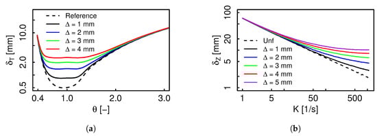
Figure 1. Flame thickness along a (a) premixed and (b) non-premixed ${\mathrm{CH}}_4$–air manifold as a function of the equivalence ratio $\theta$ and the strain rate K, respectively, for different filter sizes.

For the premixed case depicted in Figure 1a, the unfiltered flame thickness lies between [0.5–1] mm within equivalence ratio bounds $0.6\le \theta \le 1.4$. Thus, for this range the filtered flame thickness converges to a specific value as a function of the filter size, i.e., ${\delta }_{\overline{T}}=f(\Delta )$, therefore, the filtered profile transformation will be very similar for all the flamelets. Figure 1b presents the non-premixed case, where ${\delta }_Z$ significantly decreases with K, delivering a reduction of almost two orders of magnitude in the unfiltered flame thickness. Two extreme conditions exist: an almost unmodified low strained region, and a zone in which the thickness converges for all the strain rates bigger than a given threshold $K>K_{th}=f(\Delta )$, so that finally ${\delta }_{\overline{Z}}=f(\Delta ,K)$. It turns out that while for a premixed manifold a given filter size modifies the most reactive region approximately uniformly, i.e., around $\theta =1$, its effect will completely vary all over the manifold for the non-premixed condition.

The huge flame thickness variation has important consequences over the flame front resolution. For premixed FTACLES, criteria have been proposed to determine the minimum number of points to correctly resolve the gradients, and the thickness uniformity allows the numerical grid optimization to satisfy the condition. The random nature of turbulence continuously modifies the flame strain, so that a wide region of the chemical space might be accessed, and if experimental data or previous simulations are available, the bottom limit can be determined in terms of a diffusion counterflow flamelet describing a similar trajectory. However, ensuring the resolution up to this level might impose a quite elevated computational cost not necessarily justifiable, especially if the highly strained events correspond to fluctuations with respect to a mean trajectory described by a less strained flamelet. For the low strained events the flame front might be over resolved, while only a few points might be available when considering high strained ones which are also characterized by bigger model correction terms contribution.

The mesh refinement has been determined based on the kinetic energy resolution, and the impact of this discretization strategy over the model performance should be assessed.

(b)

Filtered manifold transformation

By definition the reaction progress variable evolves monotonically throughout a premixed flame. For a diffusion flame on the contrary, c attains its peak value around $Z_{st}$ and vanishes toward $Z=0$ and $Z=1$, i.e., the fuel and oxidizer streams. There are also flame variables which might present a monotonic behavior in freely propagating premixed flames, e.g., ${\mathrm{CO}}_2$, ${\mathrm{H}}_2\mathrm{O}$, and the temperature for a ${\mathrm{CH}}_4$–air mixture. Due to their different internal structures, they perform differently on the counterflow diffusion counterpart. Hence, the filtering operation not only extends and smoothens a given profile, but for non-monotonic functions it additionally decreases the peak value depending on the gradients and the filter size.

If preferential diffusion effects are neglected, the mixture fraction does not change within a planar premixed flamelet, therefore the filtering operation extends c profile physically, while its trajectory remains unmodified in Z space. For the non-premixed case on the contrary, both c and Z profiles are modified by the filtering operation. Due to c non-monotonic evolution, its filtered peak value decreases and the flamelet trajectory in the parameterized space changes. Hence, the filtered manifold undergoes a completely different transformation as a function of the considered regime. For the premixed condition, the modification of a given filtered species in the parameterized space will be determined by its degree of correlation to c, while for diffusion flames Z must additionally be taken into consideration. Figure 2 illustrates the temperature mapping variation due to the filtering operation for premixed and non-premixed manifolds. The latter is generated exclusively employing steady flamelets and no continuation method is employed after extinction takes place, which explains the incomplete description of the chemical space distinctly observed for the unfiltered case.

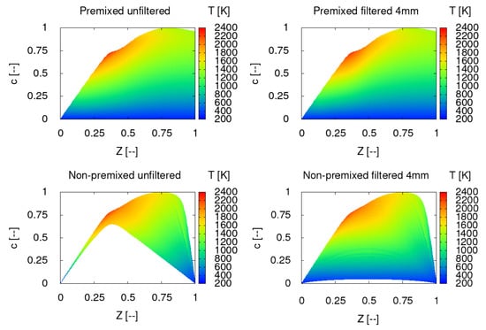
Figure 2. Temperature mapping for premixed (top) and non-premixed (bottom) manifolds.

In the premixed manifold c and T are highly correlated, the transformation undergone by the two variables is nearly identical, and the temperature is barely altered in the filtered manifold. This is a very interesting feature, because it reveals that the premixed FTACLES model affects c transport, but afterwards the flame variables will be retrieved equally either from a filtered or an unfiltered manifold. On the non-premixed manifold, the flame thickness and thus the filter sensitivity changes with K as explained above. In the upper manifold region close to chemical equilibrium, the temperature modification is marginal while for the higher strain rates, c profile is substantially clipped giving origin to a manifold extension towards the pure mixing condition, i.e., the line $c=0$. It follows that the retrieved flame variables at a given chemical space point $P_0=(Z_0,c_0)$ will change depending on the filter size. Though this behavior is fully consistent with the filtered flame structure, its comparison for instance with experimental data might be not a straightforward task. Therefore, it should first be carefully appraised considering the mean values, and subsequently for the much more challenging fluctuations prediction.

(c)

Flamelet configuration and model activation

In order to distinguish between chemically reacting and pure mixing zones, the premixed filtered or thickened flame front approaches take advantage of a flame sensor. This numerical tool handles the model activation on the former, while in the latter convection and diffusion determine the scalar transport. Definitions have been proposed, e.g., based on c [45], on its source term ${\dot{\omega }}_c$ [34], or on its gradient [49], and they can be either computed on the fly or precomputed and stored in the lookup table.

Considering that the non-premixed FTACLES model applies the filtering operation in physical space, there is a direct connection between the formalism correction terms and the chosen configuration. It follows that the one-dimensional counterflow assumption plays a major role, though the filtering principle itself is suitable to any arbitrary setup. For instance, the discrepancies between the fundamental counterflow flamelet assumptions and multidimensional phenomena found on non-premixed flames lead the non-premixed filtered tabulated chemistry model to an unphysical response as demonstrated for the case of a laminar coflow diffusion flame [35]. In this work, appropriate model performance was obtained introducing a sensor that assured the counterflow flame hypothesis through a comparison of the simulation and reference flamelet mixture fraction gradients.

The flamelet approach is a well-developed technique where the chemical representation obtained from counterflow diffusion flamelets satisfactorily captures the flame behavior. The varying flamelet thickness along the aforementioned manifold clearly affects the scalar gradients magnitude, and therefore the sensor activation in the filtered non-premixed formalism. Hence, a substantial difference between this approach and its premixed counterpart is that the model activation is not attached to a specific flame front region, but it will depend on the flame topology and mesh resolution. It is therefore necessary to assess the adequacy of the counterflow flamelet configuration for the representation of turbulent phenomena employing a filtered approach, taking into account the degree of model activation and the flexibility and smoothness between activated and deactivated conditions, to appropriately describe the real phenomena.

2.4. Description of Investigated Cases

The piloted partially premixed methane/air Sandia flames D and E configurations [50] are selected and simulated. The main jet consists of a mixture $25\%$${\mathrm{CH}}_4$ and $75\%$ air by volume, entering through a pipe with $D=7.2$ mm. The pilot stream has a diameter $D=18.2$ mm, an equivalence ratio of $\varphi =0.77$ and a temperature $T=1880$ K. The unconfined system ends with an outer air coflow at $T=291$ K. The fuel jet bulk velocity is $U_{Fuel}=49.6$ m/s and $U_{Fuel}=74.4$ m/s, and the pilot velocity $U_{Pilot}=11.4$ m/s and $U_{Pilot}=17.1$ m/s, for flames D and E, respectively. Therefore, the former presents a very small probability of local extinction which increases for the latter. Due to the high mixing rates, combustion takes place in diffusive regime with the reaction zone around the stoichiometric value. The statistical errors of the measurements for the mean major species and temperature have been reported to be below $5\%$ and those for $\mathrm{CO}$ are below $10\%$ [51].

The CFD code OpenFOAM is used with a low-Mach pressure-based approach. The combustion is addressed employing various tabulated chemistry models. The system can be considered adiabatic, therefore the thermophysical state can be fully described by means of Z and c, and no energy equation is transported. Different solvers, i.e. $lowMachNonPremFTACLESfoam$, $lowMachPremFTACLESfoam$ and $lowMachFPVfoam$, depending on each specific combustion model are employed, hence the exact formulation of Z and c equations varies as a function of the closure approach. A merged PISO-SIMPLE algorithm is applied for coupling the outer iterations, i.e., velocity, with the inner ones, i.e., pressure and the controlling variables. First, the filtered velocity is predicted employing the field variables of the previous iteration step. Then, Z and c are solved and the thermodynamic properties are updated from the tabulated database. Finally, pressure equation is solved and the velocity is corrected. Altogether six equations are solved, three for the momentum, and one for p, Z and c, respectively. In addition, the mixture fraction variance $Z_v^2$ is also solved according to the presumed $\beta$-PDF model as below specified. Turbulence generation at the inlet is based on the digital filter method by Klein et al. [52]. The WALE model [53] is used for the subgrid scale turbulence while the SGS scalar fluxes are closed either with the eddy diffusivity model or with the explicit FTACLES model terms. The employed boundary conditions are summarized in Table 2.

Table 2. Flame D and E boundary conditions. z.G stands for zero-gradient.

Stream	Z	c	U (m/s)	p (Pa)
Fuel	1	0	$U_{Fuel}$	z.G
Pilot	0.276	0.7042	$U_{Pilot}$	z.G
Coflow	0	0	0.9	z.G
Wall	z.G	z.G	0	z.G
Side	z.G	z.G	pressureInletOutletVelocity	totalPressure
Outlet	z.G	z.G	pressureInletOutletVelocity	totalPressure

The three-dimensional numerical grid schematically represented in Figure 3a is conical, non-uniform, structured with an O-grid, and consists of a pipe $L_P=13D$ and a combustion chamber $L_{ch}=80D$. Two different resolutions denoted by $M_1$ and $M_2$, respectively, are used in this study, as described in Table 3. The mesh $M_2$ results from a systematic coarsening of mesh $M_1$, with a factor close to $1.5$ in all directions, which reduces the cell number by a factor of $2.5$.

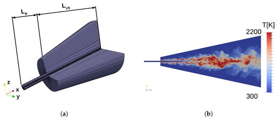
Figure 3. Sketch of the numerical mesh (a) and temperature field for Flame D (b).

Table 3. Numerical grid parameters. n is the number of divisions, the subindex $ch$ stands for chamber, p for pipe, r for radial, and L for axial direction.

Code	${\mathit{n}}_{\mathit{r},\mathbf{ch}}$	${\mathit{n}}_{\mathit{r},\mathit{p}}$	${\mathit{n}}_{\mathit{\omega }}$	${\mathit{n}}_{\mathit{L},\mathbf{ch}}$	${\mathit{n}}_{\mathit{L},\mathit{p}}$	Cells
$M_1$	143	24	17	394	145	4 Mio
$M_2$	108	15	11	329	100	1.6 Mio

The simulations are performed on the Mother High Performance Computer of the Institute of Energy and Power Plant Technology at the Technical University of Darmstadt for the phase 3 infrastructure. A decomposition into 96 processors, was used for $M_1$ and 48 processors for $M_2$. After a statistically stationary flow was obtained, the results were averaged for $0.11$ s, for which the study in [51], using the same domain length of $80D$, proved the statistics convergence.

In order to verify the mesh adequacy, as well as the inlet parameters for the turbulence generator, Flame D is initially investigated using the FPV model, before assessing the non-premixed FTACLES model. In this approach the turbulence chemistry interaction is taken into account by means of a joint subgrid PDF of Z and c. A presumed $\beta =f(Z,Z_v^2)$ is chosen for the former, while the conditional subgrid PDF $P\left(c\right|Z)$ is modeled employing a $\delta$ function for the latter as in [17]. Hence, additional to the six aforementioned transported variables the variance of the mixture fraction $Z_v^2$ is solved as well.

As will be seen in Section 3, the velocity and mixture fraction results correctly match the experiments, and the jet spreading rate is adequately predicted. The temperature profiles are compared where the experimental data are properly predicted. The numerical grid and the case settings have been successfully validated so that the FTACLES approach can be assessed.

2.5. Numerical Setup

The numerical implementation of the filtered tabulated chemistry model is conducted within the framework of the open source CFD code OpenFOAM 2.4.0. The solution of momentum, pressure and the parametrizing scalars is achieved employing the PIMPLE, i.e., merged PISO-SIMPLE, algorithm coupled with a low-Mach approach according to [54]. Second-order schemes are used for the temporal and spatial discretization.

2.6. Filtered Chemical Database

The manifolds are generated using the FGM method, solving the set of Equations (1)–(5). For the premixed case, freely propagating flames are employed, the mixture fraction is varied from the bottom to the top flammability limits, $Z=0.022$ to $Z=0.16$, respectively, in intervals of $Z=0.001$. In order to extrapolate the table beyond the flammability limits, the approach proposed by Ketelheun ([55]) is followed which considers the physical behavior of each variable in a non-reacting mixture. The species and consequently the progress variable are linearly interpolated, whilst for the density and the molar mass a hyperbolic behavior is assumed.

The non-premixed manifold is constructed with planar steady counterflow diffusion flamelets. The strain rate varies from 1 s${}^{-1}$, i.e., chemical equilibrium, up to 1082 s${}^{-1}$, i.e., the last ignited flamelet, and then 1083 s${}^{-1}$ corresponds to a pure mixing flamelet. The region between these last two conditions is covered employing unsteady flamelets. The generating strategy considers the time-dependent evolution of the last ignited flamelet towards the pure mixing condition, under a gradual strain rate increase.

The detailed chemistry solver CHEM1D [56] is used to generate the one-dimensional flamelets. The chemical evolution is described by means of the $GRI-3.0$[57] detailed chemical mechanism, with unity $Le$ assumption. The progress variable is computed according to Equation (6), the selected species i are ${\mathrm{CO}}_2$, and $\mathrm{CO}$, and the weight factor ${\gamma }_i$ equal to unity, as proposed in [58].

The filtering operation of the one-dimensional flamelet solutions is achieved by means of the Gaussian filter introduced in Equation (14). Aiming to track the flamelet giving origin to each filtered profile, a flamelet label ${\mathrm{K}}_{\mathrm{Label}}$ defined as the strain rate at the oxidizer side of the unfiltered solution is stored in the look-up table, in addition to the thermochemical quantities and the closure terms.

3. Results

The performance of the premixed and non-premixed FTACLES models is assessed on Sandia flames D and E. First, the velocity, mixture fraction and temperature profiles are presented, showing that the formalism adequately describes the flow field and the evolution of the combustion reaction. Subsequently, the species prediction, retrieved from the table is analyzed and the transformation due to the filtering operation is discussed.

3.1. Flow Field and Mixing

At the centerline, premixed and non-premixed FTACLES, and FPV deliver satisfactory results. For flame D, the start of the reaction at the centerline is slightly delayed for FTACLES in both regimes, i.e., Z and T profiles are shifted downstream, as can be seen in Figure 4. For flame E, Figure 5 indicates that non-premixed FTACLES and FPV coincide, whilst premixed FTACLES appears to better capture the temperature rise.

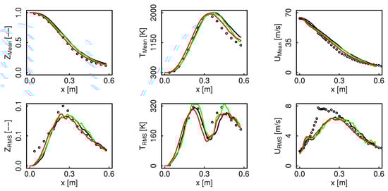
Figure 4. Flame D mixture fraction, temperature and velocity profiles along the centerline. Black color represents non-premixed FTACLES, green color premixed FTACLES, red color FPV, and circles depict the experimental data.

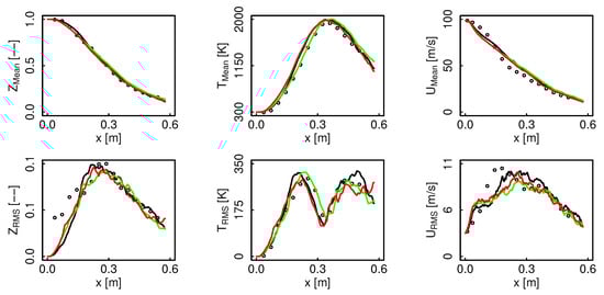
Figure 5. Flame E mixture fraction, temperature and velocity profiles along the centerline. Black color represents non-premixed FTACLES, green color premixed FTACLES, red color FPV, and circles depict the experimental data.

Figure 6 demonstrates that the mixing is correctly retrieved for the two cases with all the different models. For the non-premixed FTACLES model the mixture fraction transport is described by Equation (24), where the turbulent flux is estimated either based on a precomputed correction source term or employing a gradient diffusion hypothesis. Thus, the adequate Z profiles confirm the adequacy of the closure approach based on filtering arguments.

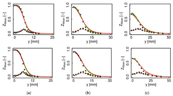
Figure 6. Mixture fraction mean and RMS radial profiles for flame D (top) and E (bottom). Black color represents non-premixed FTACLES, green color premixed FTACLES, red color FPV, solid line mean, dashed line RMS. Circles depict experimental mean, and triangles experimental RMS. (a) $x/d=7.5$; (b) $x/d=15$; (c) $x/d=30$.

The flow field is equally retrieved by all the models as it can be recognized on Figure 7. The FTACLES formalism captures the filtered flame structure by applying correction terms to the parameterizing variables transport equations, while the correction arising from the direct filtering of the momentum equation is not considered. It follows that the model impacts the flow field only indirectly, i.e., through the density and laminar viscosity values. While in RANS the laminar viscosity might play a secondary role, due to the high turbulent viscosity, in LES an appropriate estimation of the former is fundamental. Therefore, the adequate flow field description not only for the mean but also for the fluctuations confirms the consistency of the non-premixed filtered manifold transformation: the laminar viscosity is correctly estimated, so that the SGS contribution remains unmodified.

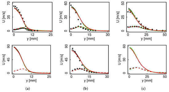
Figure 7. Velocity mean and RMS radial profiles for flame D (top) and E (bottom). Black color represents non-premixed FTACLES, green color premixed FTACLES, red color FPV, solid line mean, dashed line RMS. Circles depict experimental mean, and triangles experimental RMS. (a) $x/d=7.5$; (b) $x/d=15$; (c) $x/d=30$.

3.2. Reaction Evolution

Contrary to the mixture fraction and the flow field, the reaction evolution here scrutinized via the temperature, appears to be more sensitive to the combustion model. For flame D, both premixed and non-premixed FTACLES predict identical results and outperform the FPV model at $x/d=7.5$. This trend changes for flame E where at the above mentioned radial coordinate the premixed FTACLES and FPV better describe the experimental data, while a slight over prediction is appreciated for the non-premixed FTACLES. Further downstream the flame front becomes wider, i.e., K decreases, it can be better resolved on the computational cells and the SGS contribution decreases. Therefore, the curves are marginally distinguishable and all of the models deliver acceptable results.

The results presented in Figure 8 are quite encouraging as they demonstrate that the non-premixed FTACLES model captures a filtered flame structure which is fully consistent with the numerical grid resolution and correctly represents the physics. The varying flame thickness as a function of K along a non-premixed manifold presents a challenge for diffusion flames filtering as it might require a minimum number of points to correctly resolve the flame front, and this criterion might be more restrictive than the employed filter size. The correct reaction evolution prediction confirms the adequate flame characterization despite the varying flame thickness. This demonstrates the capacity of the formalism to handle the varying filter effect due to flame strain and retrieve a coherent resolved flame.

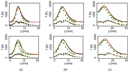
Figure 8. Temperature mean and RMS radial profiles for flame D (top) and E (bottom). Black color represents non-premixed FTACLES, green color premixed FTACLES, red color FPV, solid line mean, dashed line RMS. Circles depict experimental mean, and triangles experimental RMS. (a) $x/d=7.5$; (b) $x/d=15$; (c) $x/d=30$.

4. Discussion

The previous results showed that the non-premixed FTACLES is able to adequately capture the flow field, the mixing and the reaction evolution. This section addresses the effect of the combustion regime employed for the flamelet generation on the chemical flame structure description. Two phenomena should then be considered: the flamelet topology and the manifold transformation due to the filtering operation. The outcome proves that the non-premixed filtered model is able to appropriately retrieve the species, i.e., the filtered manifold can reproduce the experimental findings.

4.1. Chemical Source Term Transformation

The filtering operation effect in non-premixed flamelets depends on K and also on the profile thickness of every single variable. The reactive zone is therefore narrower than the whole flame, i.e., the chemical source term is very thin. The FTACLES formalism, exploits this feature so that it significantly reduces the source term magnitude and extends it over the chemical space, while it adequately depicts main flame variables.

Figure 9 and Figure 10 depict the chemical source term scattering for premixed and non-premixed FTACLES at different radial sections. Despite the different flamelet topology in the two regimes, the decrease in peak values is quite similar for both premixed and non-premixed so that the resulting values after the filtering operation indeed coincide. Due to the specificity of the configuration, i.e., in non-premixed the profile modification takes place in Z direction, the reaction zone becomes wider in this condition than in the premixed one, and this effect is more remarkable on flame E. The extension occurs toward the fuel side, and a similar response is observed for the chemical source term employing the FPV model, which further supports the idea of a characteristic counterflow flamelets manifold transformation. The distinct source term computation ties together with the model correction terms, so that finally the retrieved T almost does not change. This reinforces the previous statement, i.e., for highly strained events the resolved flame front is able to appropriately capture the flame behavior.

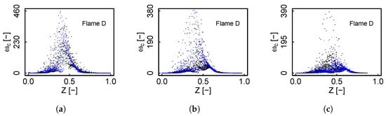
Figure 9. Progress variable chemical source term scattering at different radial sections for flame D. Black color represents non-premixed FTACLES and blue color premixed FTACLES. (a) $x/d=7.5$; (b) $x/d=15$; (c) $x/d=30$.

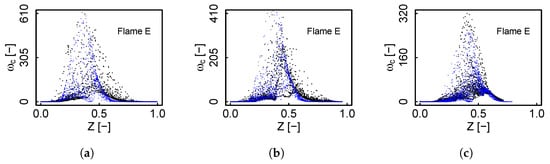
Figure 10. Progress variable chemical source term scattering at different radial sections for flame D. Black color represents non-premixed FTACLES and blue color premixed FTACLES. (a) $x/d=7.5$; (b) $x/d=15$; (c) $x/d=30$.

4.2. Species Prediction

Figure 11 and Figure 12 present different species profiles along the centerline for the premixed and non-premixed FTACLES as well as the FPV model. All of the models coincide for ${\mathrm{O}}_2$ and ${\mathrm{H}}_2\mathrm{O}$. The premixed FTACLES underestimates ${\mathrm{CO}}_2$ rise together with a higher $\mathrm{CO}$ peak, while the non-premixed formalism adequately predicts the concentrations. The clear distinction between the premixed and the non-premixed results agrees with the findings in [59]. For $\mathrm{OH}$, the FPV model appears to better capture the behavior, while the FTACLES delivers slightly higher values for both of the regimes.

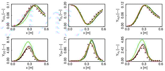
Figure 11. Species profiles comparison along the centerline for flame D. Black color represents non-premixed FTACLES, green color premixed FTACLES, red color FPV, and circles depict the experimental data.

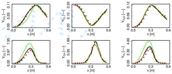
Figure 12. Species profiles comparison along the centerline for flame E. Black color represents non-premixed FTACLES, green color premixed FTACLES, red color FPV, and circles depict the experimental data.

Figure 13 and Figure 14 present ${\mathrm{H}}_2\mathrm{O}$ and ${\mathrm{O}}_2$ radial profiles. For flame D, the profiles coincide at all the sections, both for the mean and the fluctuations, while for flame E there is a difference at $x/d=7.5$ and afterwards the curves converge. This behavior coincides with the reaction evolution already depicted in Figure 8. The considered species are equally predicted in both regimes, which suggests that for this level of turbulence and employed filter, the accessed part of the manifold is analogous.

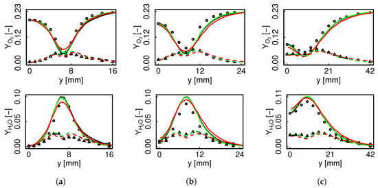
Figure 13. ${\mathrm{O}}_2$ and ${\mathrm{H}}_2\mathrm{O}$ mean and RMS radial profiles for flame D. Black color represents non-premixed FTACLES, green color premixed FTACLES, red color FPV, solid line mean, dashed line RMS. Circles depict experimental mean, and triangles represent experimental RMS. (a) $x/d=7.5$; (b) $x/d=15$; (c) $x/d=30$.

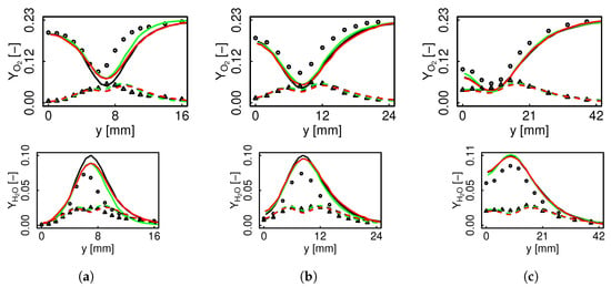
Figure 14. ${\mathrm{O}}_2$ and ${\mathrm{H}}_2\mathrm{O}$ mean and RMS radial profiles for flame E. Black color represents non-premixed FTACLES, green color premixed FTACLES, red color FPV, solid line mean, dashed line RMS. Circles depict experimental mean, and triangles represent experimental RMS. (a) $x/d=7.5$; (b) $x/d=15$; (c) $x/d=30$.

Figure 15 and Figure 16 present $\mathrm{CO}$ and ${\mathrm{CO}}_2$ profiles. There is a clear difference between the premixed and the non-premixed filtered response. In agreement with the behavior observed along the centerline, for the premixed regime $\mathrm{CO}$ concentration is overestimated resulting in lower ${\mathrm{CO}}_2$ values on the rich side of the flame, and they converge on the lean side.

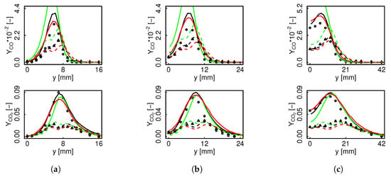
Figure 15. $\mathrm{CO}$ and ${\mathrm{CO}}_2$ mean and RMS radial profiles for flame D. Black color represents non-premixed FTACLES, green color premixed FTACLES, red color FPV, solid line mean, dashed line RMS. Circles depict experimental mean, and triangles represent experimental RMS. (a) $x/d=7.5$; (b) $x/d=15$; (c) $x/d=30$.

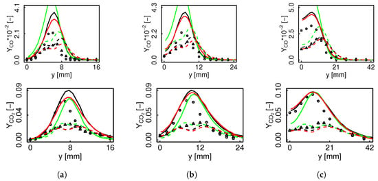
Figure 16. $\mathrm{CO}$ and ${\mathrm{CO}}_2$ mean and RMS radial profiles for flame E. Black color represents non-premixed FTACLES, green color premixed FTACLES, red color FPV, solid line mean, dashed line RMS. Circles depict experimental mean, and triangles represent experimental RMS. (a) $x/d=7.5$; (b) $x/d=15$; (c) $x/d=30$.

4.3. Filtering Effect over Non-Monotonic Species: OH

Figure 17 compares $\mathrm{OH}$ estimation between the various models for the two flames at three different radial sections. In order to assess the manifold transformation effect, $\mathrm{OH}$ has additionally been retrieved employing unfiltered premixed and non-premixed tables. The non-premixed filtered (black) and unfiltered (purple) results coincide on the mean values, while higher fluctuations are obtained with the unfiltered manifold. For the premixed case on the contrary, the unfiltered table (green) systematically surpasses the FTACLES (blue) results both for the mean and for the fluctuations.

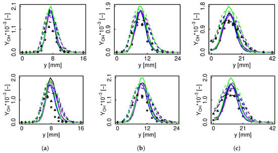
Figure 17. $\mathrm{OH}$ mean and RMS radial profiles for flame D (top) and E (bottom). Black color represents non-premixed FTACLES, blue color premixed FTACLES, purple color non-premixed unfiltered manifold, green color premixed unfiltered manifold. Solid line depicts mean, dashed line RMS, circles experimental mean, and triangles experimental RMS. (a) $x/d=7.5$; (b) $x/d=15$; (c) $x/d=30$.

For the non-premixed condition, the decrease of the fluctuations with the filtering operation reveals the manifold homogenization. The flamelets are redistributed along the chemical space, so that the most strained and therefore thinner ones approach the pure mixing line. $\mathrm{OH}$ has a narrower profile than the previously analyzed species, i.e., ${\mathrm{H}}_2\mathrm{O}$, ${\mathrm{O}}_2$, $\mathrm{CO}$ and ${\mathrm{CO}}_2$, and is therefore more sensitive to the filtering operation, and undergoes a greater modification. It follows that a fixed progress variable scattering in mixture fraction space delivers a lower $\mathrm{OH}$ variation due to the manifold smoothening. This is not observed for species having similar profile thickness than c. Altogether, a transformation in the correlation and parameterization in Z space occurs, as can be seen from $\mathrm{OH}$ behavior conditionally averaged on the mixture fraction in Figure 18. The non-premixed FTACLES model appears strikingly promising as it barely overestimates the experimental measurements after this highly complex chemical space alteration.

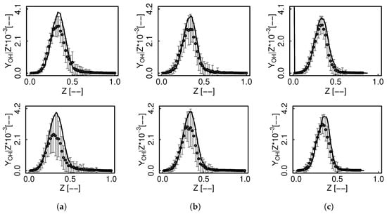
Figure 18. Non-premixed FTACLES conditional mean mass fraction of $\mathrm{OH}$ for flame D (top) and E (bottom). Solid line represents the simulation, circles the experimental data and error bars RMS. (a) $x/d=7.5$; (b) $x/d=15$; (c) $x/d=30$.

Considering the premixed tables, the difference between filtered and unfiltered results indicate the varying species filter sensitivity as an intrinsic property of the FTACLES approach, which in this regime is mostly observable for non-monotonic variables. Thus, while for ${\mathrm{H}}_2\mathrm{O}$, ${\mathrm{O}}_2$, $\mathrm{CO}$ and ${\mathrm{CO}}_2$ the differences between premixed and non-premixed results mostly obey the regime, the filter effect plays a non-negligible role in the comparison for $\mathrm{OH}$. Hence, the results presented in this section demonstrate that the non-premixed FTACLES formulation modifies the manifold in a consistent way from which the flame structure and obtained statistics can be transparently interpreted. Acknowledging the slow $\mathrm{NO}$ formation process, i.e., its large timescale which does not satisfy the high Da number hypothesis and the following overestimation by means of direct look-up table retrieval, solving a transport equation for $\mathrm{NO}$ appears to be a good alternative for coupling with the non-premixed FTACLES as in [59,60].

5. Conclusions

This study demonstrates the capability of the non-premixed FTACLES as a modeling strategy for diffusive turbulent combustion. The performance of the non-premixed FTACLES model on a turbulent flame is assessed for the first time. As application objects, the Sandia flames D and E have been selected, as they are well documented in terms of experimental data and model validation in the literature. The proposed strategy appropriately characterizes the wrinkled flame front condition as it couples the combustion formalism with an SGS modeling function. The three-dimensional tabulation methodology with explicit consideration of the numerical grid delivers satisfactory results. The model adequately portrays the underlying physics by virtue of an accurate estimation of the major stable species as well as the minor ones. Placing them into context, these results substantiate that in addition to statistical approaches, SGS closure in non-premixed combustion can be soundly represented exploiting filtering arguments.

The current study departs from an insightful description of the filtering properties as a function of the combustion regime to theorize on practical implications, and carefully analyze their repercussions on the obtained results. The effects of the filtering operation on premixed and non-premixed flamelets have been thoroughly appraised. The flame structure modification has been described considering an individual flamelet and the entire manifold. It turns out that:

• The filter effect varies considerably along the non-premixed manifold as function of K due to the flame thickness reduction at higher strain rates while it has a relatively constant effect in the zone close to stoichiometry for premixed combustion.
• The filter effect also differs for each variable within a flamelet, depending on the profile shape and thickness. As a result, there might be a non-linear relation between $Z,c$ and the retrieved species $\phi$ under the filtering operation.
• The highly varying filter sensitivity along the manifold has been identified as the biggest challenge for the non-premixed method, as it influences the response of the model correction terms, as well as the retrieved variables manifold.
• The satisfactory species prediction demonstrated the ease of interpreting the results and the practical usefulness of the method.

This work is relevant for the combustion community as it provides a clear perspective of the non-premixed FTACLES formalism possibilities and conditions for the model’s utilization and optimal performance. Due to its mathematical derivation, the model most deeply describes an unwrinkled flame front which cannot be resolved by the numerical grid, as is the case for liquid rocket engines. Furthermore, as the non-premixed FTACLES transformation results into a continuation method below the steady flamelet in mixture fraction space, the method appears as a promising alternative to model moderate flame extinction and re-ignition.

References

- Scholtissek, A.; Chan, W.L.; Xu, H.; Hunger, F.; Kolla, H.; Chen, J.H.; Ihme, M.; Hasse, C. A multi-scale asymptotic scaling and regime analysis of flamelet equations including tangential diffusion effects for laminar and turbulent flames. Combust. Flame 2015, 162, 1507–1529. [Google Scholar] [CrossRef]
- Van Oijen, J.; Donini, A.; Bastiaans, R.; ten Thije Boonkkamp, J.; De Goey, L. State-of-the-art in premixed combustion modeling using flamelet generated manifolds. Prog. Energy Combust. Sci. 2016, 57, 30–74. [Google Scholar] [CrossRef] [Green Version]
- Sacomano Filho, F.L.; Hosseinzadeh, A.; Sadiki, A.; Janicka, J. On the interaction between turbulence and ethanol spray combustion using a dynamic wrinkling model coupled with tabulated chemistry. Combust. Flame 2020, 215, 203–220. [Google Scholar] [CrossRef]
- Mahmoud, R.; Jangi, M.; Ries, F.; Fiorina, B.; Janicka, J.; Sadiki, A. Combustion Characteristics of a Non-Premixed Oxy-Flame Applying a Hybrid Filtered Eulerian Stochastic Field/Flamelet Progress Variable Approach. Appl. Sci. 2019, 9, 1320. [Google Scholar] [CrossRef] [Green Version]
- Lysenko, D.A.; Ertesvåg, I.S.; Rian, K.E. Numerical simulation of non-premixed turbulent combustion using the eddy dissipation concept and comparing with the steady laminar flamelet model. Flow Turbul. Combust. 2014, 93, 577–605. [Google Scholar] [CrossRef]
- Miranda, F.C.; Coelho, P.J.; di Mare, F.; Janicka, J. Study of turbulence-radiation interactions in large-eddy simulation of scaled Sandia flame D. J. Quant. Spectrosc. Radiat. Transf. 2019, 228, 47–56. [Google Scholar] [CrossRef]
- Dressler, L.; Filho, F.S.; Sadiki, A.; Janicka, J. Influence of Thickening Factor Treatment on Predictions of Spray Flame Properties Using the ATF Model and Tabulated Chemistry. Flow Turbul. Combust. 2020, 106, 419–451. [Google Scholar] [CrossRef]
- Pitsch, H.; Chen, M.; Peters, N. Unsteady flamelet modeling of turbulent hydrogen-air diffusion flames. In Proceedings of the Symposium (International) on Combustion, Boulder, CO, USA, 2–7 August 1998; Volume 27, pp. 1057–1064. [Google Scholar]
- Pitsch, H. Unsteady flamelet modeling of differential diffusion in turbulent jet diffusion flames. Combust. Flame 2000, 123, 358–374. [Google Scholar] [CrossRef]
- Verhoeven, L.; Ramaekers, W.; Van Oijen, J.; De Goey, L. Modeling non-premixed laminar co-flow flames using flamelet-generated manifolds. Combust. Flame 2012, 159, 230–241. [Google Scholar] [CrossRef]
- Libby, P.A.; Williams, F.A. Structure of laminar flamelets in premixed turbulent flames. Combust. Flame 1982, 44, 287–303. [Google Scholar] [CrossRef]
- Peters, N. Laminar diffusion flamelet models in non-premixed turbulent combustion. Prog. Energy Combust. Sci. 1984, 10, 319–339. [Google Scholar] [CrossRef]
- Peters, N. Turbulent combustion. Meas. Sci. Technol. 2001, 12, 2022. [Google Scholar] [CrossRef]
- van Oijen, J.A. Flamelet-Generated Manifolds: Development and Application to Premixed Laminar Flames; Technische Universiteit Eindhoven: Eindhoven, The Netherlands, 2002. [Google Scholar]
- Poinsot, T.; Veynante, D. Theoretical and Numerical Combustion; RT Edwards, Inc.: Bundaberg, QLD, Australia, 2005. [Google Scholar]
- Cook, A.W.; Riley, J.J.; Kosály, G. A laminar flamelet approach to subgrid-scale chemistry in turbulent flows. Combust. Flame 1997, 109, 332–341. [Google Scholar] [CrossRef]
- Pierce, C.D.; Moin, P. Progress-variable approach for large-eddy simulation of non-premixed turbulent combustion. J. Fluid Mech. 2004, 504, 73–97. [Google Scholar] [CrossRef]
- Ihme, M.; Cha, C.M.; Pitsch, H. Prediction of local extinction and re-ignition effects in non-premixed turbulent combustion using a flamelet/progress variable approach. Proc. Combust. Inst. 2005, 30, 793–800. [Google Scholar] [CrossRef]
- Nishioka, M.; Law, C.; Takeno, T. A flame-controlling continuation method for generating S-curve responses with detailed chemistry. Combust. Flame 1996, 104, 328–342. [Google Scholar] [CrossRef]
- Wu, H.; Ihme, M. Modeling of wall heat transfer and flame/wall interaction a flamelet model with heat-loss effects. In Proceedings of the 9th US National Combustion Meeting, Cincinnati, OH, USA, 17–20 May 2015; pp. 17–20. [Google Scholar]
- Wen, X.; Luo, K.; Luo, Y.; Kassem, H.I.; Jin, H.; Fan, J. Large eddy simulation of a semi-industrial scale coal furnace using non-adiabatic three-stream flamelet/progress variable model. Appl. Energy 2016, 183, 1086–1097. [Google Scholar] [CrossRef]
- Coclite, A.; Pascazio, G.; De Palma, P.; Cutrone, L.; Ihme, M. An SMLD joint PDF model for turbulent non-premixed combustion using the flamelet progress-variable approach. Flow Turbul. Combust. 2015, 95, 97–119. [Google Scholar] [CrossRef] [Green Version]
- Bushe, W.K.; Steiner, H. Laminar flamelet decomposition for conditional source-term estimation. Phys. Fluids 2003, 15, 1564–1575. [Google Scholar] [CrossRef]
- Emami, M.; Fard, A.E. Laminar flamelet modeling of a turbulent CH4/H2/N2 jet diffusion flame using artificial neural networks. Appl. Math. Model. 2012, 36, 2082–2093. [Google Scholar] [CrossRef]
- Gicquel, O.; Darabiha, N.; Thévenin, D. Liminar premixed hydrogen/air counterflow flame simulations using flame prolongation of ILDM with differential diffusion. Proc. Combust. Inst. 2000, 28, 1901–1908. [Google Scholar] [CrossRef]
- Veynante, D.; Poinsot, T. Reynolds averaged and large eddy simulation modeling for turbulent combustion. In New Tools in Turbulence Modelling; Springer: Berlin/Heidelberg, Germany, 1997; pp. 105–140. [Google Scholar]
- Colin, O.; Ducros, F.; Veynante, D.; Poinsot, T. A thickened flame model for large eddy simulations of turbulent premixed combustion. Phys. Fluids 2000, 12, 1843–1863. [Google Scholar] [CrossRef]
- Hosseinzadeh, A.; Sadiki, A.; Janicka, J. Assessment of the dynamic SGS wrinkling combustion modeling using the thickened flame approach coupled with FGM tabulated detailed chemistry. Flow Turbul. Combust. 2016, 96, 939–964. [Google Scholar] [CrossRef]
- Kuenne, G.; Ketelheun, A.; Janicka, J. LES modeling of premixed combustion using a thickened flame approach coupled with FGM tabulated chemistry. Combust. Flame 2011, 158, 1750–1767. [Google Scholar] [CrossRef]
- Rittler, A.; Proch, F.; Kempf, A.M. LES of the Sydney piloted spray flame series with the PFGM/ATF approach and different sub-filter models. Combust. Flame 2015, 162, 1575–1598. [Google Scholar] [CrossRef]
- Fiorina, B.; Vicquelin, R.; Auzillon, P.; Darabiha, N.; Gicquel, O.; Veynante, D. A filtered tabulated chemistry model for LES of premixed combustion. Combust. Flame 2010, 157, 465–475. [Google Scholar] [CrossRef] [Green Version]
- Charlette, F.; Meneveau, C.; Veynante, D. A power-law flame wrinkling model for LES of premixed turbulent combustion Part II: Dynamic formulation. Combust. Flame 2002, 131, 181–197. [Google Scholar] [CrossRef]
- Charlette, F.; Meneveau, C.; Veynante, D. A power-law flame wrinkling model for LES of premixed turbulent combustion Part I: Non-dynamic formulation and initial tests. Combust. Flame 2002, 131, 159–180. [Google Scholar] [CrossRef]
- Schmitt, T.; Sadiki, A.; Fiorina, B.; Veynante, D. Impact of dynamic wrinkling model on the prediction accuracy using the F-TACLES combustion model in swirling premixed turbulent flames. Proc. Combust. Inst. 2013, 34, 1261–1268. [Google Scholar] [CrossRef]
- Obando Vega, P.J.; Coussement, A.; Sadiki, A.; Parente, A. Non-Premixed Filtered Tabulated Chemistry: Filtered Flame Modeling of Diffusion Flames. Fuels 2021, 2, 87–107. [Google Scholar] [CrossRef]
- De Goey, L.; ten Thije Boonkkamp, J. A flamelet description of premixed laminar flames and the relation with flame stretch. Combust. Flame 1999, 119, 253–271. [Google Scholar] [CrossRef]
- De Goey, L.; ten Thije Boonkkamp, J. A mass-based definition of flame stretch for flames with finite thickness. Combust. Sci. Technol. 1997, 122, 399–405. [Google Scholar] [CrossRef]
- Ramaekers, W.; Van Oijen, J.; De Goey, L. A priori testing of flamelet generated manifolds for turbulent partially premixed methane/air flames. Flow Turbul. Combust. 2010, 84, 439–458. [Google Scholar] [CrossRef] [Green Version]
- Donini, A.; Bastiaans, R.; van Oijen, J.; De Goey, L. Differential diffusion effects inclusion with flamelet generated manifold for the modeling of stratified premixed cooled flames. Proc. Combust. Inst. 2015, 35, 831–837. [Google Scholar] [CrossRef]
- Mercier, R.; Auzillon, P.; Moureau, V.; Darabiha, N.; Gicquel, O.; Veynante, D.; Fiorina, B. Les modeling of the impact of heat losses and differential diffusion on turbulent stratified flame propagation: Application to the tu darmstadt stratified flame. Flow Turbul. Combust. 2014, 93, 349–381. [Google Scholar] [CrossRef]
- Mercier, R.; Schmitt, T.; Veynante, D.; Fiorina, B. The influence of combustion SGS submodels on the resolved flame propagation. Application to the LES of the Cambridge stratified flames. Proc. Combust. Inst. 2015, 35, 1259–1267. [Google Scholar] [CrossRef] [Green Version]
- Auzillon, P.; Gicquel, O.; Darabiha, N.; Veynante, D.; Fiorina, B. A filtered tabulated chemistry model for LES of stratified flames. Combust. Flame 2012, 159, 2704–2717. [Google Scholar] [CrossRef]
- Philip, M.; Boileau, M.; Vicquelin, R.; Riber, E.; Schmitt, T.; Cuenot, B.; Durox, D.; Candel, S. Large Eddy Simulations of the ignition sequence of an annular multiple-injector combustor. Proc. Combust. Inst. 2015, 35, 3159–3166. [Google Scholar] [CrossRef] [Green Version]
- Pope, S.B. Turbulent Flows; Cornell University: New York, NY, USA, 2001. [Google Scholar]
- Durand, L.; Polifke, W. Implementation of the thickened flame model for large eddy simulation of turbulent premixed combustion in a commercial solver. In Proceedings of the ASME Turbo Expo 2007: Power for Land, Sea, and Air, Montreal, QC, Canada, 14–17 May 2007; pp. 869–878. [Google Scholar]
- Coussement, A.; Schmitt, T.; Fiorina, B. Filtered Tabulated Chemistry for non-premixed flames. Proc. Combust. Inst. 2015, 35, 1183–1190. [Google Scholar] [CrossRef]
- Wang, L. Analysis of the filtered non-premixed turbulent flame. Combust. Flame 2017, 175, 259–269. [Google Scholar] [CrossRef] [Green Version]
- Veynante, D.; Vervisch, L. Turbulent combustion modeling. Prog. Energy Combust. Sci. 2002, 28, 193–266. [Google Scholar] [CrossRef]
- Proch, F.; Kempf, A.M. Numerical analysis of the Cambridge stratified flame series using artificial thickened flame LES with tabulated premixed flame chemistry. Combust. Flame 2014, 161, 2627–2646. [Google Scholar] [CrossRef]
- Barlow, R.; Frank, J. Piloted CH4/Air Flames C, D, E, and F—Release 2.1. 15 June 2007. Available online: https://tnfworkshop.org/wp-content/uploads/2019/02/SandiaPilotDoc21.pdf (accessed on 23 June 2016).
- Ihme, M.; Pitsch, H. Modeling of radiation and nitric oxide formation in turbulent nonpremixed flames using a flamelet/progress variable formulation. Phys. Fluids 2008, 20, 055110. [Google Scholar] [CrossRef] [Green Version]
- Klein, M.; Sadiki, A.; Janicka, J. A digital filter based generation of inflow data for spatially developing direct numerical or large eddy simulations. J. Comput. Phys. 2003, 186, 652–665. [Google Scholar] [CrossRef]
- Nicoud, F.; Ducros, F. Subgrid-scale stress modelling based on the square of the velocity gradient tensor. Flow Turbul. Combust. 1999, 62, 183–200. [Google Scholar] [CrossRef]
- Ries, F.; Obando, P.; Shevchuck, I.; Janicka, J.; Sadiki, A. Numerical analysis of turbulent flow dynamics and heat transport in a round jet at supercritical conditions. Int. J. Heat Fluid Flow 2017, 66, 172–184. [Google Scholar]
- Ketelheun, A.; Olbricht, C.; Hahn, F.; Janicka, J. Premixed generated manifolds for the computation of technical combustion systems. In Proceedings of the ASME Turbo Expo 2009: Power for Land, Sea, and Air, Orlando, FL, USA, 8–12 June 2009; pp. 695–705. [Google Scholar]
- Somers, B. The Simulation of Flat Flames with Detailed and Reduced Chemical Models. Ph.D. Thesis, Eindhoven University of Technology, Eindhoven, The Netherlands, 1994. [Google Scholar]
- Smith, G.P. GRI-3.0. 2000. Available online: http://www.me.berkeley.edu/gri_mech/ (accessed on 15 March 2017).
- Fiorina, B.; Baron, R.; Gicquel, O.; Thevenin, D.; Carpentier, S.; Darabiha, N. Modelling non-adiabatic partially premixed flames using flame-prolongation of ILDM. Combust. Theory Model. 2003, 7, 449–470. [Google Scholar] [CrossRef]
- Vreman, A.; Albrecht, B.; Van Oijen, J.; De Goey, L.; Bastiaans, R. Premixed and nonpremixed generated manifolds in large-eddy simulation of Sandia flame D and F. Combust. Flame 2008, 153, 394–416. [Google Scholar] [CrossRef]
- Donini, A.; Bastiaans, R.; van Oijen, J.; de Goey, L. A 5-D implementation of FGM for the large eddy simulation of a stratified swirled flame with heat loss in a gas turbine combustor. Flow Turbul. Combust. 2017, 98, 887–922. [Google Scholar] [CrossRef] [Green Version]
Publisher’s Note: MDPI stays neutral with regard to jurisdictional claims in published maps and institutional affiliations. |
© 2022 by the authors. Licensee MDPI, Basel, Switzerland. This article is an open access article distributed under the terms and conditions of the Creative Commons Attribution (CC BY) license (https://creativecommons.org/licenses/by/4.0/).