Article

Fault Diagnosis Method Using CNN-Attention-LSTM for AC/DC Microgrid

1
State Grid Jiangsu Electric Power Co., Ltd., Research Institute, Nanjing 211103, China
2
College of Artificial Intelligence and Automation, Hohai University, Nanjing 210098, China
3
State Grid Jiangsu Electric Power Co., Ltd., Nanjing 210024, China
*
Author to whom correspondence should be addressed.
Modelling 2025, 6(3), 107; https://doi.org/10.3390/modelling6030107
Submission received: 27 August 2025 / Revised: 14 September 2025 / Accepted: 15 September 2025 / Published: 18 September 2025

Abstract

From the perspectives of theoretical design and practical application, the existing fault diagnosis methods with the complex identification process owing to manual feature extraction and the insufficient feature extraction for time series data and weak fault signal is not suitable for AC/DC microgrids. Thus, this paper proposes a fault diagnosis method that integrates a convolutional neural network (CNN) with a long short-term memory (LSTM) network and attention mechanisms. The method employs a multi-scale convolution-based weight layer (Weight Layer 1) to extract features of faults from different dimensions, performing feature fusion to enrich the fault characteristics of the AC/DC microgrid. Additionally, a hybrid attention block-based weight layer (Weight Layer 2) is designed to enable the model to adaptively focus on the most significant features, thereby improving the extraction and utilization of critical information, which enhances both classification accuracy and model generalization. By cascading LSTM layers, the model effectively captures temporal dependencies within the features, allowing the model to extract critical information from the temporal evolution of electrical signals, thus enhancing both classification accuracy and robustness. Simulation results indicate that the proposed method achieves a classification accuracy of up to 99.5%, with fault identification accuracy for noisy signals under 10 dB noise interference reaching 92.5%, demonstrating strong noise immunity.

1. Introduction

The increasing integration of power electronic equipment has led to a heightened probability of faults in AC/DC microgrids. Consequently, these faults propagate more rapidly, and there exists significant variations in the magnitude, direction, and duration of fault currents [1,2,3,4,5,6]. Therefore, accurate fault diagnosis is essential for ensuring the safety, reliability, and stability of AC/DC microgrids.
Traditional methods for power system fault diagnosis can be categorized into two main types. The first category comprises classical model-based methods, the most significant of which are impedance detection [7,8,9,10,11,12] and traveling wave detection [13,14,15,16]. These methods have been widely utilized by grid personnel for fault diagnosis over the past few decades. However, both methods exhibit lower efficiency in AC and DC microgrids. In the case of impedance detection, fault resistance and feedthrough from distributed generation (DG) can adversely affect the measured impedance, while transient currents may also lead to inaccurate readings [17,18,19]. The traveling wave method suffers from accuracy issues due to the relatively short lengths of microgrid lines, as traveling wave signals propagate over limited distances, leading to rapid signal attenuation and complicating the detection of fault-generated traveling waves [20]. The second category encompasses machine learning data-driven methods, where scholars have employed expert systems, Bayesian networks, Petri nets, support vector machines [21,22,23,24,25], and other techniques to address grid fault diagnosis. The feature selection and dimensionality reduction techniques, principal component analysis (PCA) and random forest (RF), have been applied to active low-voltage distribution grid (LVDG) in [26,27], respectively. In [28], a multi-layer perceptron (MLP) combined with an extreme learning machine (ELM) is specifically utilized for radial grid topologies. Deep neural networks (DNNs) are employed in [29] to identify fault location and type in radial LVDG topologies. However, traditional machine learning often requires manual feature design and selection, which heavily relies on domain knowledge. If feature extraction is inadequate, model performance will be significantly constrained, and its generalization capability will be weak.
Benefit from its ability to generalize bias and extract feature, the convolutional neural network (CNN) has been developed for grid fault identification. In a previous study [30], a CNN based on continuous wavelet transform and Bayesian-optimized error parameters was employed for fault identification and type classification. The frequency domain features were extracted by Short Time Fourier Transform (STFT), and the time-frequency feature image was constructed with the time-domain data, and then the DC-CNN was used for fault identification in [31]. However, the above method used manual feature extraction, which not only requires high feature extraction algorithms, but also increases the amount of computation and complicates the fault identification process. The feature extraction algorithms are demanding and increase the computational complexity. In fact, neural networks such as the CNN have the ability to extract features automatically and can be used to identify faults on raw data samples of three-phase voltage and current. Although in [32,33] the method of automatic feature extraction was also adopted, the fact that the data collected through the sensor has a high degree of temporal sequence and nonlinearity was ignored. In addition, the temporal feature extraction of the data is still insufficient to handle the power data collected by the sensors. LSTM is an efficient temporal feature extraction tool with powerful modeling capabilities to capture long-term dependencies, automatically learn time-dependent features, and effectively cope with the gradient vanishing problem, making it excellent in areas such as bearing fault detection and lifetime prediction. In [34], the combination of a 1-D CNN and LSTM has been shown to outperform not only traditional methods but also other similar deep learning networks in classification and regression tasks. In addition, since the current limiting control of power electronic devices in AC/DC microgrids can weaken the fault features and make it difficult to recognize them directly, there is an urgent need to improve the capability of the CNN in feature extraction and fault detection to enhance the accuracy of capturing and recognizing the weak fault features and to improve the reliability and robustness of fault diagnosis [35,36,37]. The proposed visual attention mechanism [38,39,40,41,42], which simulates human cognition, has proven to be equally effective in extracting fault features. The attention mechanism can adaptively adjust weights to emphasize subtle changes in these features. Ukwuoma et al. integrated a multi-scale attention network into a deep graph neural network, incorporating spatial features during the training process, thereby enabling the model to gain a richer topological understanding from the data and exhibit stronger resilience to anomalous data and changing environments [43]. Overall, the attention mechanism provides a robust solution to these challenges by leveraging all the information in the feature graph to enhance overall model performance.
Based on the above discussion, the research gap from the perspectives of theoretical design and practical application can be summarized as follows.
(1)
Conventional machine learning methods for fault diagnosis of AC/DC microgrid rely on manual feature extraction algorithms, which not only increases the amount of computation but also complicates the fault identification process.
(2)
Existing fault identification methods do not possess sufficient capability to extract the time series features of the data, which have difficulty in dealing with the power data collected by the sensors.
(3)
Influenced by the current-limiting control of power electronic devices in AC/DC microgrids, some faults present weak characteristics, which have not been considered seriously by the existing strategy.
Inspired by the above discussion, this paper proposes a fault identification method based on CNN-Attention-LSTM, which is mainly used to diagnose fault types in AC-DC hybrid microgrids. By integrating the CNN, hybrid attention mechanism, and LSTM, a fault identification model is constructed. The weighting layer I is centered on multi-scale convolution to extract local features at different scales, while the weighting layer II consists of the hybrid attention mechanism to enhance the weights of important features. The LSTM layer handles the time series data. The method utilizes the measured three-phase voltage and current information to effectively discriminate faults and is applicable to AC and DC microgrid networks with multiple DGs.
The main contributions of the proposed approach include the following:
(1)
Unlike model-based approaches that rely on accurate system modeling and struggle with parameter uncertainties, CAL directly learns from operational data, enhancing robustness under nonlinear and dynamic conditions.
(2)
In previous machine learning studies [14,44], manual feature extraction algorithms were utilized before the fault identification, which is not conductive to practical applications. The method proposed in this paper eliminates the manual feature extraction and simplifies the identification process.
(3)
In the field of fault diagnosis of the AC/DC microgrid, the input data, including voltage and current collected by sensors, possesses temporal characteristics, which cannot be mined using the existing CNN [17,45]. In this paper, we introduce the LSTM layer combined into the CNN, which can capture long-term dependencies and automatically learn time-related features.
(4)
Due to the fact that the current limiting control of power electronic devices in the AC/DC microgrid weakens fault features, there is an urgent need to improve the existing technology to increase the accuracy of recognizing tiny fault features. Different with the CNN in [46], a hybrid attention mechanism is integrated to focus subtle changes in these features so that the fault diagnosis performance can be enhanced for the AC/DC microgrid.

2. CNN-Attention-LSTM Modeling

The network structure of the CNN-Attention-LSTM (CAL) fault diagnosis model is shown in Figure 1. For the input three-phase voltage and current signals, high-dimensional and low-dimensional features are first extracted through Weight Layer 1. These features are then passed through Weight Layer 2, where the feature weights are assigned. Subsequently, the LSTM layer, centered on the LSTM network, processes the data. These two modules are cascaded sequentially, thoroughly exploring data features from both multidimensional perspectives and temporal dependencies.

2.1. Multi-Scale Parallel Convolutional Networks

The CNN is a widely used neural network for processing time series data, primarily composed of convolutional layers, pooling layers, and fully connected layers. To extract more effective fault features, a multi-scale parallel convolutional layer is introduced as Weight Layer 1, allowing the extraction of features from different dimensions.
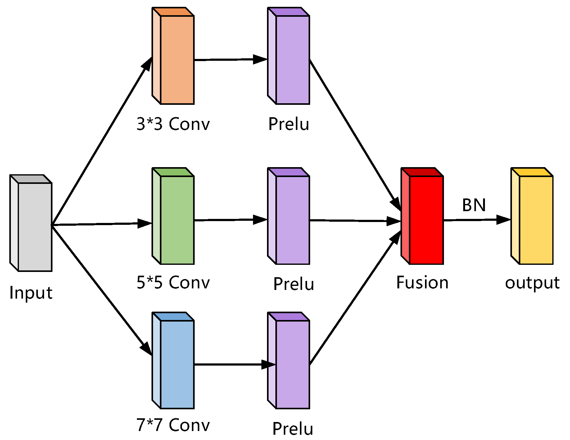
Weight Layer 1 employs parallel stacks of 3 × 3, 5 × 5, and 7 × 7 convolutional layers to extract local features from the input data. A feature fusion module then integrates the multi-scale information to produce an output with enhanced representational capacity. The structure of Weight Layer 1 is shown in Figure 2.
As can be seen in Figure 2, the AC/DC microgrid fault features are extracted from three convolution sizes. The convolution kernel of size 3 × 3 is employed to extract low-dimensional feature information, while the 5 × 5 convolution kernel and the 7 × 7 convolution kernel are utilized to obtain high-dimensional feature information. The output of the convolutional layer is described as
Y c = f ( X W τ + b τ )
where X denotes the raw input data, W τ = { W 3 τ , W 5 τ , W 7 τ } denotes the weights of the first multi-scale parallel convolution kernel, b τ = { b 3 τ , b 5 τ , b 7 τ } are the bias terms, and denotes the convolution operator. Since the three-phase voltage and three-phase current have a large number of negative channel parts, PReLU is utilized as the activation function instead of ReLU [47], defined as
PReLU ( x i ) = x i , if   x i > 0 α i x i , if   x i 0
where x i represents the feature information of the i t h channel; α i controls the slope of the negative part of the first channel. In addition, α i is a learnable parameter that can be updated simultaneously with other layers through backpropagation, thus enhancing the model expressiveness.
In order to enrich the fault characterization information of AC and DC microgrids, we fuse features from several different convolutional kernels. This process is called fusion layer in this paper. Assuming that the feature in the fusion layer is C , it can be defined as
C = f W 3 r * X + b 3 r + f W 5 r * X + b 5 r + f ( W 7 r * X + b 7 r ) = Y c 3 + Y c 5 + Y c 7
From (3), it can be seen that the fusion layer has stronger fault characteristics than each of the convolutional kernel layers. These three different scales complement each other and provide more complete fault characterization information, even if one of the features is weaker, and are used as inputs to the next layer of the hybrid attention module.

2.2. Convolutional Block Attention Module (CBAM)

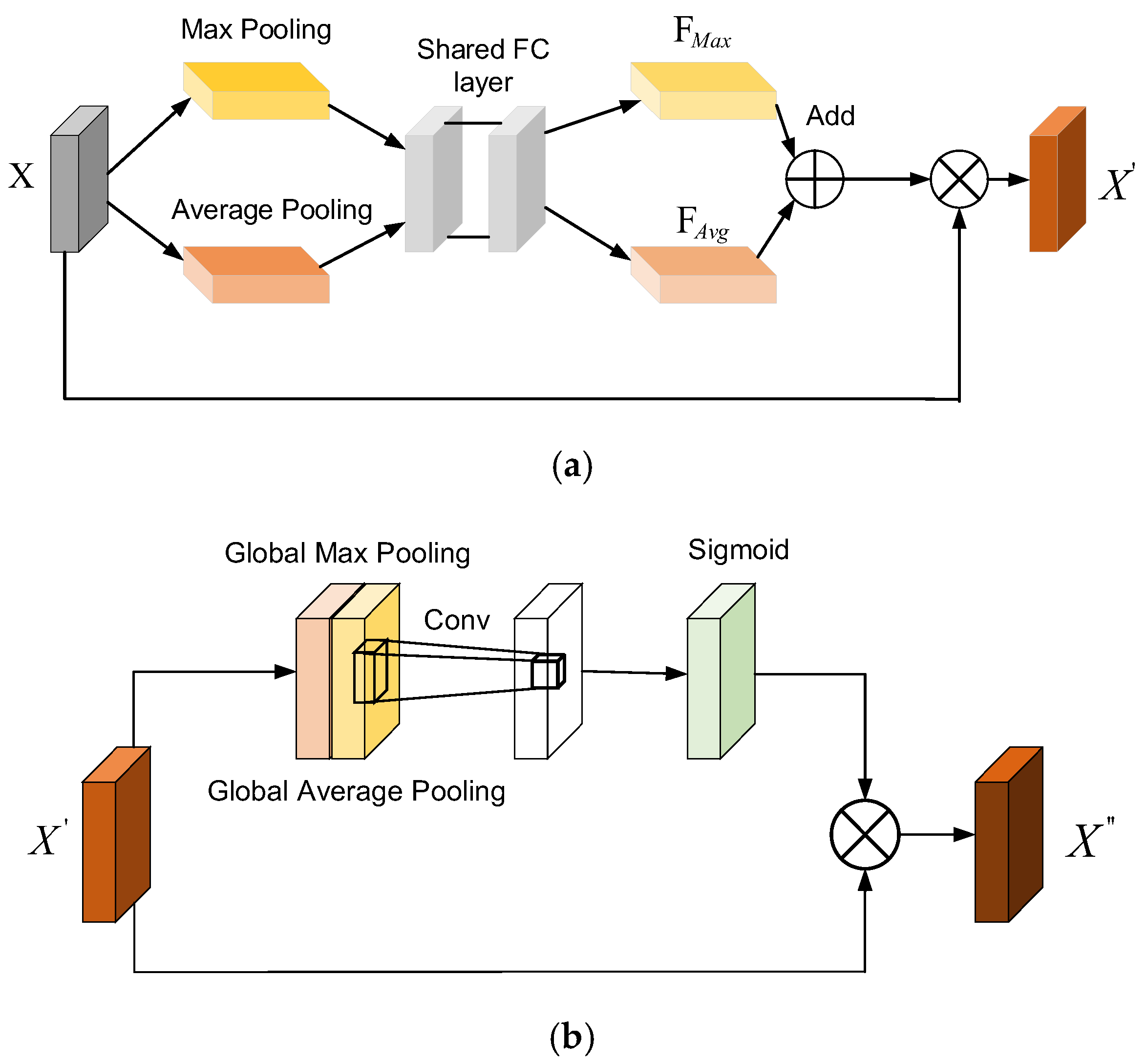
Different from the traditional CNN, the main goal of weight layer 2 in CAL is to significantly improve the representation of fault features provided by Weight Layer 1. Inspired by Woo et al. in [48], the attention module is positioned after the fusion layer as Weight Layer 2, employing a combination of maximum pooling and average pooling for aggregating the attention module, thereby minimizing the loss of fault feature information. The design of Weight Layer 2 in CAL is shown in Figure 3.
The channel attention module highlights the features that are important for the classification task by learning the weights of each channel, thus suppressing unimportant features. This enables the model to concentrate more effectively on information relevant for fault classification, improving classification accuracy.
The input feature map provided by the weighting layer 1 k F T × C , where T is the time step of the sample and C is the number of channels of the sample, is extracted through the average pooling layer and the maximum pooling layer, which denote the integrated feature information and the unique feature information, respectively, and the pooling results are passed through two fully connected layers.
The output dimension of the first fully connected layer is c r , where r is the compression ratio, usually taken as 8. The first Shared FC layer:
F avg = f ( W 1 X avg + b 1 ) F max = f ( W 1 X max + b 1 )
where W 1 C × C r , b 1 C r , f ( ) is the PReLU function. F avg represents the feature map of the average pooling layer; F max and represents the feature map of the max pooling layer.
The second Shared FC layer:
F avg = W 2 F avg + b 2 F max = W 2 F max + b 2
The outputs of the two FC layers are summed and then passed through the sigmoid activation function; F channel = σ ( F avg + F max ) , which denotes the sigmoid activation function. The input feature map is multiplied with the channel attention weights to obtain a weighted feature map:
X = X F channel
where denotes the element-by-point multiplication.
The spatial attention module performs global average pooling and global maximum pooling on the channel-weighted feature maps X to obtain two single-channel feature maps X a v g ' and X max ' . The results of average pooling and maximum pooling are spliced:
X concat = Concat ( X avg , X max )
where X concat T × 2 .
A convolution operation is performed on the spliced feature map to obtain the spatial attention weights:
F spatial = σ ( Conv 1 D ( X concat ) )
where F spatial T × 1 , σ denotes the sigmoid activation function.
The input feature map is multiplied with the spatial attention weights to obtain a weighted feature map:
X = X F spatial
where ⊙ denotes the element-by-point multiplication.
From the above introduction, the spatial attention module can improve the effect of feature extraction by focusing on important locations in the input feature map, enabling the model to capture key spatial information more accurately, and by combining with the channel attention module it can make full use of all the information in the feature map to improve the overall performance of the model.

2.3. LSTM Layer

LSTM networks represent an enhancement of recurrent neural networks (RNNs). By incorporating three specialized gate structures and a memory unit [49], they address the short-term memory issue inherent in RNNs, where distant information exerts negligible influence on the current time step due to gradient vanishing.
In Figure 3, X t denotes the input at time t, h t denotes the hidden layer output at time step, C t denotes the memory cell at time t, C ˜ t denotes the temporary memory cell, ⊗ denotes element-wise multiplication, and ⊕ denotes element-wise addition. The forget gate adds information to the current memory cell C t , while the output gate controls the output result of memory cell C t . The computational process is as follows:
f t = σ ( W f [ h t 1 , x t ] + b f ) i t = σ ( W i [ h t 1 , x t ] + b i ) C ˜ t = tanh ( W C ˜ [ h t 1 , x t ] + b C ˜ ) C t = f t C t 1 i t C ˜ t o t = σ ( W o [ h t 1 , x t ] + b o ) h t = o t tanh C t
where W f , W i , W C ˜ , W o represent the weight matrix corresponding to each module; b f , b i , b C ˜ , b o denote the bias term, σ is the sigmoid activation function, and tanh is the hyperbolic tangent activation function.
The LSTM layer is applied to the convolutional feature maps following the CBAM. Convolution layers are typically employed to extract local features, whilst the LSTM layer captures the temporal dependencies within these features. This approach associates the high-level features extracted by the convolutional layers with historical time series, thereby enhancing the model’s comprehension of sequential data. It facilitates a more effective capture of temporal correlations within the sequence data and improves classification performance.

3. Fault Feature Extraction and Data Processing

3.1. Fault Dataset Construction

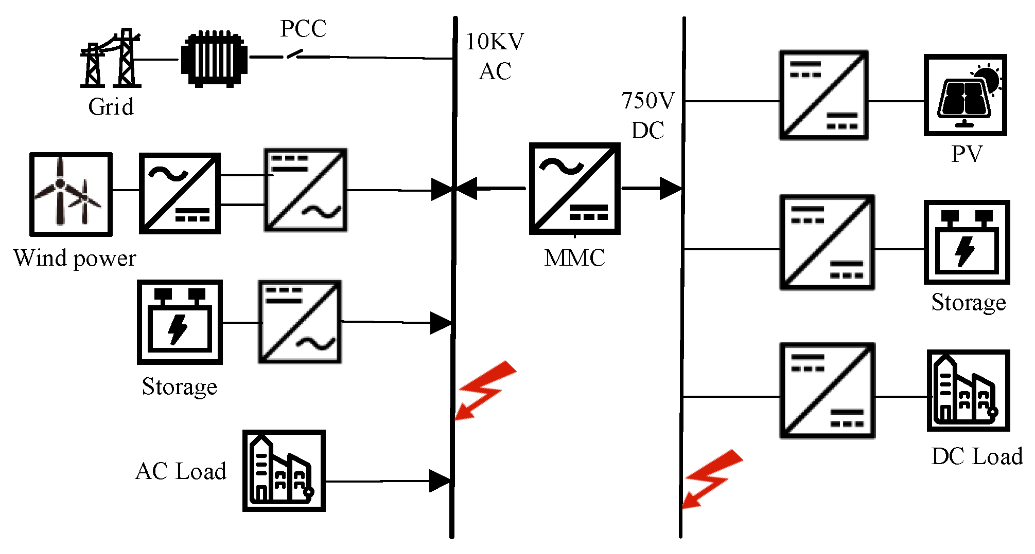
The AC/DC hybrid microgrid model was developed using PSCAD V4.6. This model comprises an AC subnet, a DC subnet, and an interconnected converter, as illustrated in Figure 4 and Table 1. In this topology, the AC bus connects to the distribution network via a transformer, while the DC bus connects to the AC bus through a modular multilevel converter (MMC). Wind power generation, energy storage, and AC loads are linked to the AC bus, whereas photovoltaic generation, energy storage, and DC loads are associated with the DC bus.
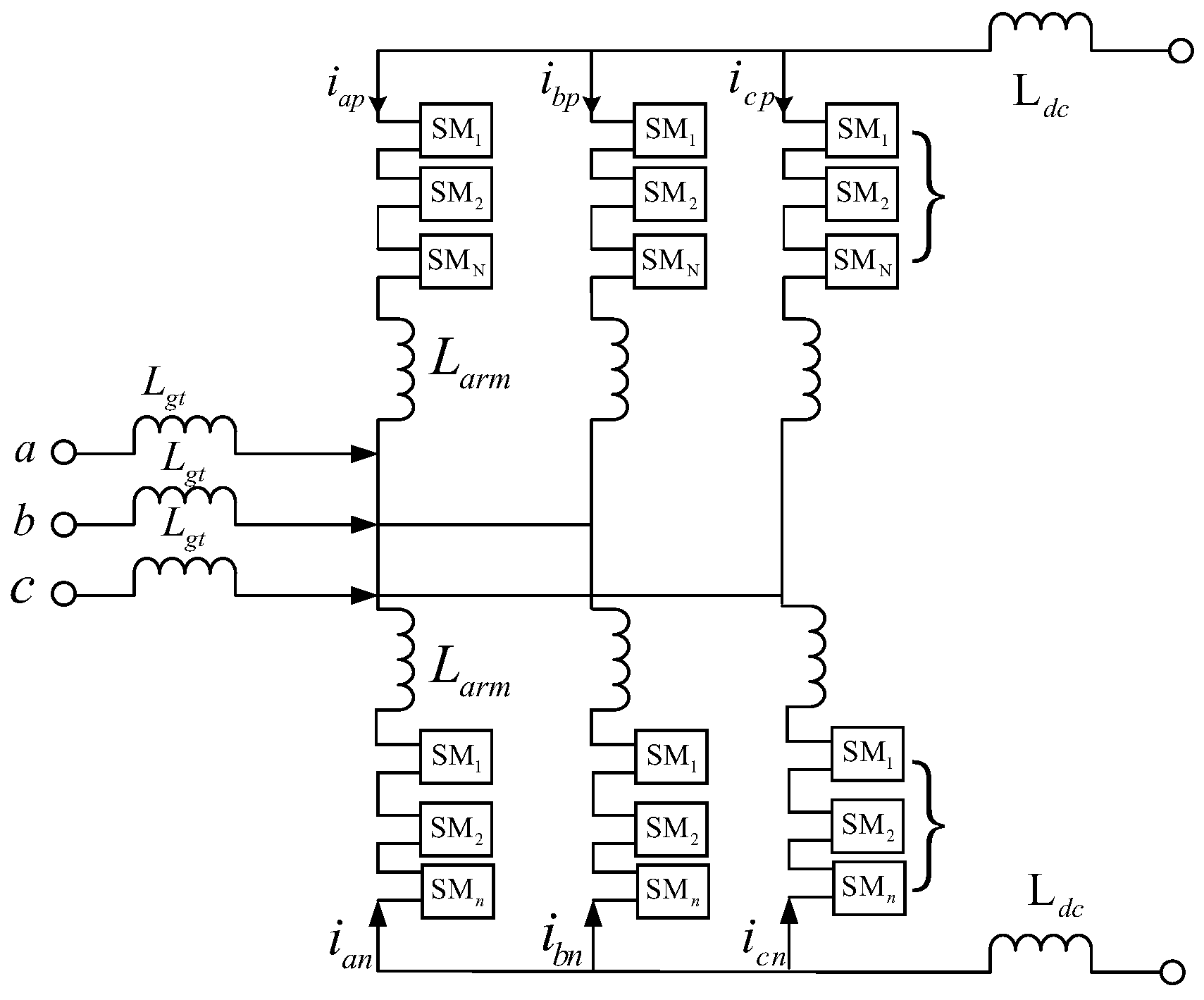
The considered power converter in the AC/DC microgrid is a half-bridge MMC, as shown in Figure 5. The half-bridge submodule is made up of two IGBTs and a DC capacitor, controlled by complementary signals. This configuration generates two operating states, which can either commit or bypass the corresponding capacitors, producing a multilevel waveform output. The DC capacitors act as energy buffers and constant voltage sources.

3.2. Fault Data Processing

The study conducted simulations of the AC/DC microgrid, encompassing both normal operating conditions and nine fault scenarios. The three-phase currents and voltages are measured at the point of common coupling (PCC) during faults, providing the corresponding current and voltage for each phase.
The collected three-phase voltage and current data have different scales. Common methods include Min-Max normalization and Z-score normalization. In this paper, the Min-Max normalization method is utilized to process the data. This study collected a total of 1000 samples, ensuring an even distribution across categories. To evaluate the effectiveness of the fault diagnosis approach, the dataset is divided into training and testing subsets. We opted for a random allocation of data in an 8:2 ratio to maintain a balance between training and testing.
Faults in AC/DC hybrid microgrids can be classified into two categories: AC-side faults and DC-side faults. In this paper, 10 different types of faults are set up, including single-phase ground faults (A-G, B-G, C-G), phase-to-phase short circuits (AB-G, BC-G, AC-G), three-phase ground short circuits (ABC-G), and single-phase ground (P-G) and phase-to-phase short circuits (P-P).
Fault locations are set at the AC and DC buses, respectively, and the measurement points for all faults are at the PCC (point of common coupling). The simulations are conducted after the AC/DC microgrid has been running normally for 1 s, with the fault duration set to 0.2 s, and the fault sampling frequency is set to 10 kHz. The specific sample distribution is shown in Table 2.

4. Simulation Validation

4.1. Fault Diagnosis with Clean Data

In the experiments for the ten fault diagnosis types presented in Table 2, the model hyperparameters are set as follows: Weight Layer 1 consists of 64 multi-scale convolutional layers, and the LSTM layer contains 128 nodes in its hidden layer. The learning rate is optimized using the ReduceLROnPlateau method, with a minimum learning rate of 0.0001. The total number of iterations is set to 200, and the batch size is configured at 64. Sparse Categorical Cross entropy is selected as the loss function. The configuration of the computer used is as follows: Processor: AMD R7 7745HX, Graphics: NVIDIA GeForce RTX 4060 Laptop GPU, Memory: 32 GB DDR5–5600.
For a sample i , its true label is y i { 0 , 1 , , C 1 } , and the predicted probability vector p i = ( p i , 0 , p i , 1 , , p i , C 1 ) , where p i , c denotes the predicted probability of class c .
The sparse categorical cross-entropy loss is defined as follows:
Loss i = log ( p i , y i )
The overall loss (averaged over N samples) is
Loss = 1 N i = 1 N log ( p i , y i )
The corresponding accuracy is given by
Accuracy = 1 N i = 1 N 1 ( arg max c p i , c = y i ) ,
where 1 ( ) is the indicator function, which equals 1 if the predicted class matches the true label, and 0 otherwise.
Loss and accuracy are two independent evaluation metrics, not complementary measures. Accuracy denotes the proportion of correctly classified samples relative to the total sample size, typically expressed as a percentage. Loss values, however, are computed via a predefined loss function (such as cross-entropy for sparse classes), which measures the deviation between the predicted probability distribution and the true labels. As loss values represent a continuous measure reflecting both prediction confidence and error magnitude, they do not necessarily exhibit a linear relationship with accuracy. Consequently, the sum of loss values and accuracy does not equal 100%.
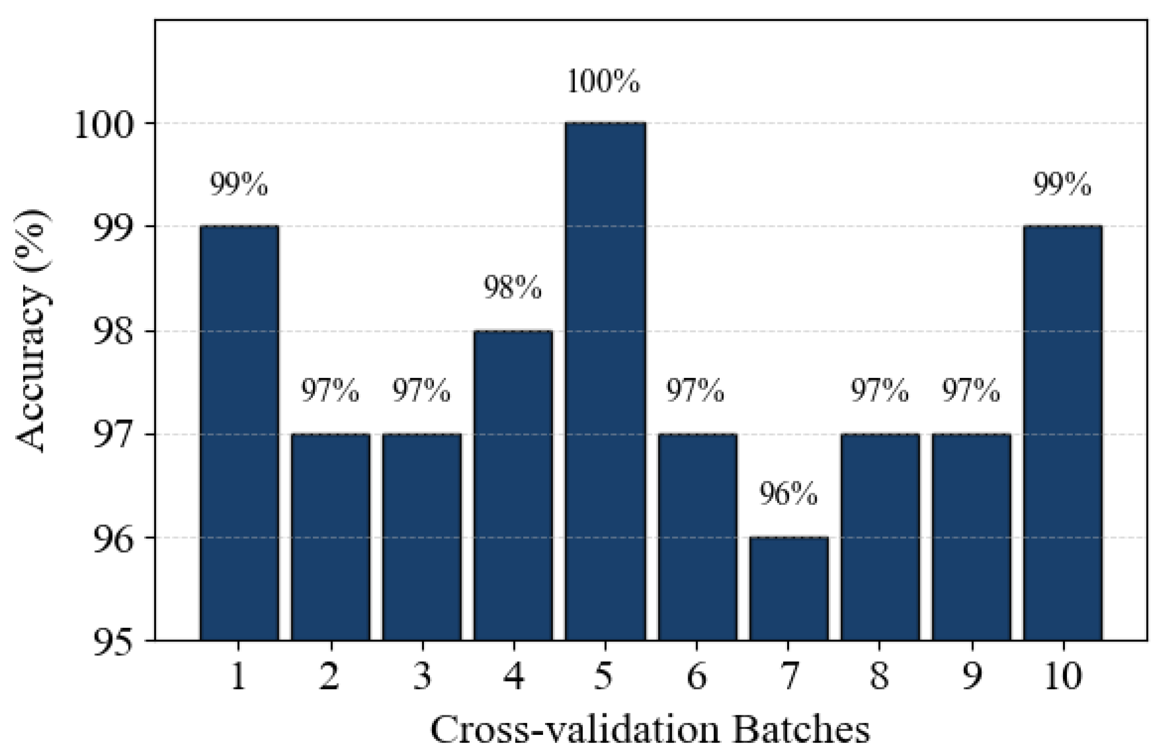
In the 10-fold cross-validation experiments [50], the model achieves a maximum accuracy of 100% and a minimum accuracy of 96%, with an average accuracy of 97.77%. This indicates that the model’s performance is stable across different data subsets and demonstrates robustness against overfitting. Figure 6 illustrates the accuracy of the model on the test set for each fold.
Dividing the training and test sets according to the ratio of 8:2, Figure 7 shows the trend of the model’s accuracy and loss during the training process. As the number of iterations increases, the model’s loss gradually decreases and approaches zero, while the accuracy on the training set rises steadily. Through extensive experimentation, we found that the model performs optimally after 200 iterations, achieving a training accuracy of 99.69% and a loss value of 0.019. On the test set, the model’s accuracy reaches 99.5%.

4.2. Comparison Analysis

To validate the superiority of the proposed CNN-Attention-LSTM (CAL) model for fault diagnosis in AC/DC microgrid models, we compared our model with commonly used models, including the CNN and SVM. In this comparison, the CNN model shares the same multi-scale convolutional layers in Weight Layer 1 as our proposed model. The test results are presented in Table 3, while the confusion matrices are illustrated in Figure 8.
As shown in Table 3, the CNN-Attention-LSTM (CAL) model achieves the highest average accuracy on the test set, reaching 99.50%. The SVM and CNN models have comparable average accuracies, indicating that the attention mechanism enhances the upper limit of classification accuracy. The faults that the CNN and SVM cannot correctly deal with mainly include single-pole ground fault and pole-to-pole short circuits fault on the DC side. From the perspective of PCC, the current derived from single-pole ground and pole-to-pole short circuit is similar. Due to the limitation of model structure, the CNN and SVM cannot capture local information (e.g., anomalies in the signal at a certain moment), global information (e.g., overall signal trends), and the temporal correlations in the sequence data, so it is difficult to identify the faults with similar shapes.
Although the attention mechanism in the CAL model slightly increases computational complexity, it can still complete the accurate diagnosis within 2 ms, albeit with a slightly slower speed compared to the CNN and SVM structures.
In summary, the proposed model effectively combines the strengths of the CNN and the attention mechanism, facilitating comprehensive extraction of both low-dimensional and high-dimensional features from the data. This capability enables thorough exploration of feature information, resulting in accurate fault classification. Additionally, the model meets the objective of rapid diagnosis, ensuring timely fault detection.

4.3. Anti-Interference Analysis

Given that real-world sampled data often includes noise, fault characteristics are prone to being masked by these interferences. Therefore, it is essential to evaluate the performance of the proposed fault diagnosis method under noisy conditions. Gaussian noise is added to the original signal to create composite signals with varying signal-to-noise ratios (SNRs).
We added Gaussian white noise to the samples in both the training and test sets, and tested the models under different signal-to-noise ratios (SNRs). The results are shown in Figure 9.
Based on the test results, it can be observed that as the noise intensity increases, the accuracy of the model on the test set gradually decreases. CAL achieves the highest accuracy of 98% at 40 dB and the lowest accuracy of 92.5% at 10 dB. As shown in Figure 9, CAL exhibits better noise robustness compared to the SVM and CNN. Therefore, CAL can effectively mitigate noise interference to a certain extent, demonstrating strong noise resistance and that it is well-suited to handle noise impacts in the data acquisition process of AC-DC microgrids.

4.4. Applicability Analysis Against New Topology

To verify the applicability of the proposed CAL, a park AC/DC microgrid in a specific region, as shown in Figure 10, is used as a test prototype. This topology encompasses electric vehicles (EVs), adjustable load, distributed photovoltaic systems, and energy storage devices. The specific parameters are detailed in Table 4. For the considered AC/DC microgrid, the following fault types are defined: (1) disconnection faults: disconnection of the fixed load; (2) short-circuit and grounding faults at different locations, including the 380 V AC bus and the 1 kV DC bus; and (3) power fluctuations due to equipment faults: abnormal PV output power. Specifically, for abnormal PV output power, two fluctuation ranges are defined: 20% increase and 20% decrease. Therefore, this test example establishes 13 fault types.
The test results are collected in Table 5. It can be observed that, despite new fault types and fault locations set in the new topology, the performance deviation of the proposed CAL is quite trivial, in which it has shown superior accuracy to the CNN and SVM, significantly. For example, the accuracy of CAL is almost 98% for new topology with different noise. Conversely, the accuracy of the CNN decreases to 92%, and the SVM even decreases to 89%, further demonstrating the applicability of the proposed method.
Compared to Topology 1, Topology 2 captures a broader spectrum of fault types across multiple locations while accounting for abnormal photovoltaic output scenarios. However, whilst this study demonstrates the model’s universality within representative and practically relevant scenarios, it does not guarantee robustness across all microgrid configurations. Distinct fault characteristics may emerge when topologies feature significantly divergent converter configurations, control schemes, or higher penetration levels of distributed energy resources. Consequently, subsequent research will conduct cross-topology transfer learning experiments for broader validation, rigorously establishing the model’s universal applicability.

5. Discussion

Employing multi-scale convolutions in Weight Layer 1 typically captures diverse fault characteristics effectively, as it extracts features across varying temporal and frequency scales. This enables the model to identify local transient phenomena while also capturing the typical wide-area dynamic patterns characteristic of AC/DC microgrids. As demonstrated in Equation (3), multi-scale convolutions can enrich fault information within AC/DC microgrids. In contrast, single-scale convolutions may overlook subtle features, whilst dilated convolutions carry the risk of losing fine-grained details.
The channel attention mechanism places greater emphasis on significant channels, specifically data exhibiting more pronounced fault characteristics. For instance, in the case of a Phase A ground fault, it focuses more on Phase A current and Phase A voltage. The spatial attention mechanism places greater emphasis on critical locations, specifically moments where fault characteristics are more pronounced. For instance, short-circuit faults often exhibit particularly noticeable changes within the first few cycles, whereas some ground faults only show significant alterations in the subsequent cycles.
Regarding the trade-off between efficiency and accuracy, the primary considerations are practical factors such as hardware computational capabilities and specific requirements. In real-time deployment scenarios for embedded systems, lightweight models like Support Vector Machines (SVMs) offer outstanding efficiency but exhibit significant performance degradation under complex fault conditions. When computational complexity and real-time performance become paramount considerations, optimization strategies such as model pruning, quantization, or hardware acceleration must be employed to ensure the feasibility of the CAL framework. This approach effectively narrows the efficiency gap without substantially compromising diagnostic advantages.
Reducing model complexity is crucial for practical deployment in real-time and resource-constrained environments. Techniques such as pruning and lightweight convolutions can significantly reduce memory footprint, inference latency, and energy consumption, enabling device-side deployment without reliance on high-performance servers. However, these strategies carry inherent risks. Excessive pruning may eliminate parameters critical for representing subtle yet diagnostically valuable fault features, particularly in faults exhibiting weak characteristics. This leads to diminished model accuracy, increased false alarm rates, and compromised reliability in real-world engineering applications.
There still exists improvement room for CAL. To enhance the convenience of on-chip implementation, lightweight techniques such as model pruning and depth-separable convolution will be explored in our future study. In addition, other complex topologies, such as cluster microgrids, can be further investigated to validate the applicability of the proposed method.

6. Conclusions

To address the issue of insufficient accuracy in existing fault diagnosis methods for AC-DC microgrids, a fault diagnosis method based on CNN-Attention-LSTM is proposed. The research results are obtained as follows: (1) A fault diagnosis model based on CAL is developed by combining multi-scale convolution with hybrid attention block and LSTM, which improves the feature mining capability and acquire better fault classification accuracy. (2) The diagnosis accuracy using the proposed CAL under different noise is better than its rivals, including the CNN and SVM, which demonstrates that the proposed CAL possesses a superior robustness owing to its strong feature mining capability. (3) Under the new topology condition, the diagnosis accuracy of CAL almost contains 98% with different noise, further demonstrating the applicability of the proposed method.

Author Contributions

Methodology: Q.B., P.L., and R.S.; writing—original draft preparation: Q.B., P.L., and R.S.; writing—review and editing: Q.B., P.L., R.S., J.J., Z.L., and S.H. All authors have read and agreed to the published version of the manuscript.

Funding

This work is supported by the Science and technology project of State Grid Jiangsu Electric Power Co., Ltd., grant number. J2024024.

Data Availability Statement

The original contributions presented in this study are included in the article. Further inquiries can be directed to the corresponding author.

Conflicts of Interest

Author Qiangsheng Bu was employed by the company Electric Power Research Institute, State Grid Jiangsu Electric Power Co., Ltd., authors Pengpeng Lyu, Jiangping Jing and Zhan Lyu were employed by the company State Grid Jiangsu Electric Power Co., Ltd. The remaining authors declare that the research was conducted in the absence of any commercial or financial relationships that could be construed as a potential conflict of interest.

References

  1. Pradhan, R.; Jena, P. An innovative fault direction estimation technique for AC microgrid. Electr. Power Syst. Res. 2023, 215, 108997. [Google Scholar] [CrossRef]
  2. Lu, Z.; Wang, L.; Wang, P. Microgrid Fault Detection Method Based on Lightweight Gradient Boosting Machine–Neural Network Combined Modeling. Energies 2024, 17, 2699. [Google Scholar] [CrossRef]
  3. Montoya, R.; Poudel, B.P.; Bidram, A.; Reno, M.J. DC microgrid fault detection using multiresolution analysis of traveling waves. Int. J. Electr. Power Energy Syst. 2022, 135, 107590. [Google Scholar] [CrossRef]
  4. Pola, S.; Azzouz, M.A.; Mirhassani, M. Synchronverters with fault ride-through capabilities for reliable microgrid protection during balanced and unbalanced faults. IEEE Trans. Sustain. Energy 2024, 15, 1663–1676. [Google Scholar] [CrossRef]
  5. Vinayagam, A.; Suganthi, S.; Venkatramanan, C.; Alateeq, A.; Alassaf, A.; Ab Aziz, N.F.; Mansor, M.H.; Mekhilef, S. Discrimination of high impedance fault in microgrid power network using semi-supervised machine learning algorithm. Ain Shams Eng. J. 2025, 16, 103187. [Google Scholar] [CrossRef]
  6. Mohan, F.; Sasidharan, N. Protection of low voltage DC microgrids: A review. Electr. Power Syst. Res. 2023, 225, 109822. [Google Scholar] [CrossRef]
  7. Ghzaiel, W.; Ghorbal, M.J.-B.; Slama-Belkhodja, I.; Guerrero, J.M. Grid impedance estimation based hybrid islanding detection method for AC microgrids. Math. Comput. Simul. 2017, 131, 142–156. [Google Scholar] [CrossRef]
  8. Fang, M.; Zhang, D.; Qi, X. Real-Time Voltage Drop Compensation Method With Cable Impedance Detection Capability for Remote Power Supply Systems. IEEE Trans. Power Electron. 2023, 38, 9322–9328. [Google Scholar] [CrossRef]
  9. Yadegar, M.; Zarei, S.F.; Meskin, N.; Blaabjerg, F. A distributed high-impedance fault detection and protection scheme in DC microgrids. IEEE Trans. Power Deliv. 2023, 39, 141–154. [Google Scholar] [CrossRef]
  10. Hamatwi, E.; Imoru, O.; Kanime, M.M.; Kanelombe, H.S.A. Comparative analysis of high impedance fault detection techniques on distribution networks. IEEE Access 2023, 11, 25817–25834. [Google Scholar] [CrossRef]
  11. Alaei, S.A.; Damchi, Y. A new method based on the discrete time energy separation algorithm for high and low impedance faults detection in distribution systems. Electr. Power Syst. Res. 2023, 218, 109200. [Google Scholar] [CrossRef]
  12. Dubey, K.; Jena, P. Impedance angle-based differential protection scheme for microgrid feeders. IEEE Syst. J. 2020, 15, 3291–3300. [Google Scholar] [CrossRef]
  13. Saleh, K.; Hooshyar, A.; El-Saadany, E.F. Fault detection and location in medium-voltage DC microgrids using travelling-wave reflections. IET Renew. Power Gener. 2020, 14, 571–579. [Google Scholar] [CrossRef]
  14. Chen, H.; Li, J.; Chen, P. Design of fault location algorithm based on online distributed travelling wave for HV power cable. PLoS ONE 2024, 19, e0296513. [Google Scholar]
  15. Sahoo, B.; Samantaray, S.R. An enhanced travelling wave-based fault detection and location estimation technique for series compensated transmission network. In Proceedings of the 2017 7th International Conference on Power Systems (ICPS), Pune, India, 21–23 December 2017. [Google Scholar]
  16. Kumar, R.; Tripathy, M. A novel impedance based fault locator algorithm for transmission line. Electr. Power Syst. Res. 2023, 224, 109731. [Google Scholar] [CrossRef]
  17. Bhargav, R.; Gupta, C.P.; Bhalja, B.R. Unified impedance-based relaying scheme for the protection of hybrid AC/DC microgrid. IEEE Trans. Smart Grid 2021, 13, 913–927. [Google Scholar] [CrossRef]
  18. Zhang, G.; Shi, M.; Zhang, C.; Sha, H.; She, C. Harmonic impedance detection based on capacitor switching and wavelet packet analysis. In Proceedings of the 2019 IEEE 9th Annual International Conference on CYBER Technology in Automation, Control, and Intelligent Systems (CYBER), Suzhou, China, 29 July–2 August 2019. [Google Scholar]
  19. Couto, V.F.; Moreto, M. High impedance fault detection on microgrids considering the impact of VSC based generation. IEEE Access 2023, 11, 89550–89560. [Google Scholar] [CrossRef]
  20. Saleh, K.A.; Hooshyar, A.; El-Saadany, E.F. Ultra-high-speed traveling-wave-based protection scheme for medium-voltage DC microgrids. IEEE Trans. Smart Grid 2017, 10, 1440–1451. [Google Scholar] [CrossRef]
  21. Kiaei, I.; Lotfifard, S. Fault section identification in smart distribution systems using multi-source data based on fuzzy Petri nets. IEEE Trans. Smart Grid 2019, 11, 74–83. [Google Scholar] [CrossRef]
  22. Zhou, J.; Xiao, M.; Niu, Y.; Ji, G. Rolling Bearing Fault Diagnosis Based on WGWOA-VMD-SVM. Sensors 2022, 22, 6281–6308. [Google Scholar] [CrossRef]
  23. Chauhan, V.K.; Dahiya, K.; Sharma, A. Problem formulations and solvers in linear SVM: A review. Artif. Intell. Rev. 2019, 52, 803–855. [Google Scholar] [CrossRef]
  24. Nie, F.; Zhu, W.; Li, X. Decision Tree SVM: An extension of linear SVM for non-linear classification. Neurocomputing 2020, 401, 153–159. [Google Scholar] [CrossRef]
  25. Zidan, A.; Khairalla, M.; Abdrabou, A.M.; Khalifa, T.; Shaban, K.; Abdrabou, A.; El Shatshat, R.; Gaouda, A.M. Fault detection, isolation, and service restoration in distribution systems: State-of-the-art and future trends. IEEE Trans. Smart Grid 2016, 8, 2170–2185. [Google Scholar] [CrossRef]
  26. Yan, J.; Li, Q.; Duan, S. A simplified current feature extraction and deployment method for DC series arc fault detection. IEEE Trans. Ind. Electron. 2023, 71, 625–634. [Google Scholar] [CrossRef]
  27. Li, B.; Cheng, T.; Jiang, Q.; Su, X.; Zhang, J.; Zhang, H. Faulty Feeders Identification for Single-phase-to-ground Fault Based on Multi-features and Machine Learning. IEEE Trans. Ind. Appl. 2023, 59, 7259–7270. [Google Scholar] [CrossRef]
  28. Mamuya, Y.D.; Lee, Y.-D.; Shen, J.-W.; Shafiullah, M.; Kuo, C.-C. Application of machine learning for fault classification and location in a radial distribution grid. Appl. Sci. 2020, 10, 4965. [Google Scholar] [CrossRef]
  29. Sapountzoglou, N.; Lago, J.; De Schutter, B.; Raison, B. A generalizable and sensor-independent deep learning method for fault detection and location in low-voltage distribution grids. Appl. Energy 2020, 276, 115299. [Google Scholar] [CrossRef]
  30. Arévalo, P.; Cano, A.; Benavides, D.; Jurado, F. Fault analysis in clustered microgrids utilizing SVM-CNN and differential protection. Appl. Soft Comput. 2024, 164, 112031. [Google Scholar] [CrossRef]
  31. Rizeakos, V.; Bachoumis, A.; Andriopoulos, N.; Birbas, M.; Birbas, A. Deep learning-based application for fault location identification and type classification in active distribution grids. Appl. Energy 2023, 338, 120932. [Google Scholar] [CrossRef]
  32. Korkmaz, D.; Acikgoz, H. An efficient fault classification method in solar photovoltaic modules using transfer learning and multi-scale convolutional neural network. Eng. Appl. Artif. Intell. 2022, 113, 104959. [Google Scholar] [CrossRef]
  33. Liu, H.; Liu, S.; Zhao, J.; Bi, T.; Yu, X. Dual-channel convolutional network-based fault cause identification for active distribution system using realistic waveform measurements. IEEE Trans. Smart Grid 2022, 13, 4899–4908. [Google Scholar] [CrossRef]
  34. Swaminathan, R.; Mishra, S.; Routray, A.; Swain, S.C. A CNN-LSTM-based fault classifier and locator for underground cables. Neural Comput. Appl. 2021, 33, 15293–15304. [Google Scholar] [CrossRef]
  35. Kok, C.L.; Ho, C.K.; Aung, T.H.; Koh, Y.Y.; Teo, T.H. Transfer learning and deep neural networks for robust intersubject hand movement detection from EEG signals. Appl. Sci. 2024, 14, 8091. [Google Scholar] [CrossRef]
  36. Aviña-Corral, V.; Rangel-Magdaleno, J.d.J.; Barron-Zambrano, J.H.; Rosales-Nuñez, S. Review of fault detection techniques in power converters: Fault analysis and diagnostic methodologies. Measurement 2024, 234, 114864. [Google Scholar] [CrossRef]
  37. Bhatnagar, M.; Yadav, A.; Swetapadma, A.; Abdelaziz, A.Y. LSTM-based low-impedance fault and high-impedance fault detection and classification. Electr. Eng. 2024, 106, 6589–6613. [Google Scholar]
  38. Vaswani, A. Attention is all you need. In Proceedings of the 31st International Conference on Neural Information Processing Systems, Long Beach, CA, USA, 4–9 December 2017. [Google Scholar]
  39. de Santana Correia, A.; Colombini, E.L. Attention, please! A survey of neural attention models in deep learning. Artif. Intell. Rev. 2022, 55, 6037–6124. [Google Scholar] [CrossRef]
  40. Guo, Z.; Zhang, P.; Liang, P. SAKD: Sparse attention knowledge distillation. Image Vis. Comput. 2024, 146, 105020. [Google Scholar] [CrossRef]
  41. Su, E.; Cai, S.; Xie, L.; Li, H.; Schultz, T. STAnet: A spatiotemporal attention network for decoding auditory spatial attention from EEG. IEEE Trans. Biomed. Eng. 2022, 69, 2233–2242. [Google Scholar] [CrossRef]
  42. Jiang, B.; Lu, Y.; Chen, X.; Lu, X.; Lu, G. Graph attention in attention network for image denoising. IEEE Trans. Syst. Man Cybern. Syst. 2023, 53, 7077–7088. [Google Scholar] [CrossRef]
  43. Ukwuoma, C.C.; Cai, D.; Bamisile, O.; Chukwuebuka, E.J.; Favour, E.; Emmanuel, G.S.; Caroline, A.; Abdi, S.F. Power transmission system’s fault location, detection, and classification: Pay close attention to transmission nodes. Int. J. Electr. Power Energy Syst. 2024, 156, 109771. [Google Scholar] [CrossRef]
  44. Karthick, R.; Saravanan, R.; Arulkumar, P. Fault Detection and Fault Location in a Grid-Connected Microgrid Using Optimized Deep Learning Neural Network. Optim. Control Appl. Methods 2024, 46, 896–911. [Google Scholar] [CrossRef]
  45. Bukhari, S.B.A.; Kim, C.-H.; Mehmood, K.K.; Haider, R.; Zaman, M.S.U. Convolutional neural network-based intelligent protection strategy for microgrids. IET Gener. Transm. Distrib. 2020, 14, 1177–1185. [Google Scholar] [CrossRef]
  46. Siddique, M.N.I.; Shafiullah; Mekhilef, S.; Pota, H.; Abido, M.A. Fault classification and location of a PMU-equipped active distribution network using deep convolution neural network (CNN). Electr. Power Syst. Res. 2024, 229, 110178. [Google Scholar] [CrossRef]
  47. Ma, J.; Tang, Q.; He, M.; Peretto, L.; Teng, Z. Complex PQD Classification Using Time–Frequency Analysis and Multiscale Parallel Attention Residual Network. IEEE Trans. Ind. Electron. 2024, 71, 9658–9667. [Google Scholar] [CrossRef]
  48. Woo, S.; Park, J.; Lee, J.Y.; Kweon, I.S. Cbam: Convolutional block attention module. In Proceedings of the European Conference on Computer Vision (ECCV), Munich, Germany, 8–14 September 2018. [Google Scholar]
  49. Hochreiter, S. Long Short-term Memory. Neural Comput. 1997, 9, 1735–1780. [Google Scholar] [CrossRef]
  50. Fu, W.J.; Carroll, R.J.; Wang, S. Estimating misclassification error with small samples via bootstrap cross-validation. Bioinformatics 2005, 21, 1979–1986. [Google Scholar] [CrossRef] [PubMed]
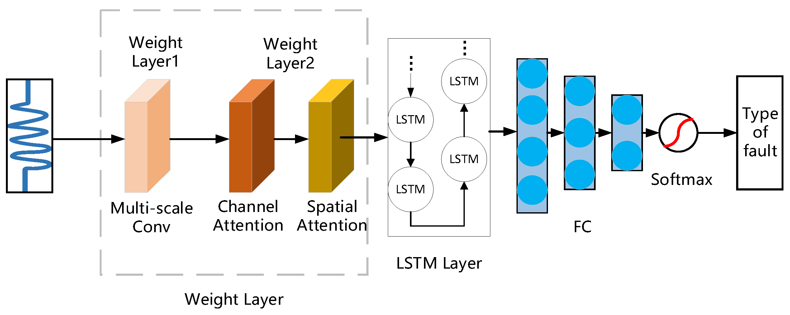
Figure 1. CAL network structure.
Modelling 06 00107 g001
Figure 2. Structure of Weight Layer 1.
Modelling 06 00107 g002
Figure 3. Structure of Weight Layer 2., (a) channel attention; (b) spatial attention.
Modelling 06 00107 g003
Figure 4. AC/DC microgrid topology.
Modelling 06 00107 g004
Figure 5. Half-bridge MMC.
Modelling 06 00107 g005
Figure 6. The 10-fold cross-validation results.
Modelling 06 00107 g006
Figure 7. Training process curve.
Modelling 06 00107 g007
Figure 8. Confusion matrices of different models. (a) CNN. (b) SVM.
Modelling 06 00107 g008
Figure 9. Performance with different noise levels against other models.
Modelling 06 00107 g009
Figure 10. Park AC/DC microgrid topology.
Modelling 06 00107 g010
Table 1. The parameters of AC/DC microgrids.
ParameterValue
Transformation ratio10/0.38 kV
Transformer power20 MVA
DC voltage750 V
Photovoltaic power0.2 MW
Turbine power0.2 MW
capacity10 MVA
AC voltage10 kV
Submodule capacitance20 mF
Bridge Arm inductors1 mH
Number of submodules100
Table 2. Distribution of collected samples.
Fault LabelSample Size
A-G100
B-G100
C-G100
AB-G100
AC-G100
BC-G100
ABC-G100
P-N100
P-P100
Normal100
Table 3. Comparison of performance among different models.
Model NameAccuracy (%)Time (s/Sample)
CAL99.51.9 × 10−3
CNN96.51.44 × 10−3
SVM967.8 × 10−4
Table 4. System parameter of the park AC/DC microgrid.
ParameterValue
Transformation ratio10/0.38 kV
Transformer power10 MVA
DC voltage1 kV
Photovoltaic power0.2 MW
Frequency50 Hz
Table 5. Performance test with new topology.
ModelAccuracy (%)
Clean40 dB20 dB10 dB
CAL98.8598.4698.4697.69
CNN969594.6292.69
SVM9594.2393.4689.23
Disclaimer/Publisher’s Note: The statements, opinions and data contained in all publications are solely those of the individual author(s) and contributor(s) and not of MDPI and/or the editor(s). MDPI and/or the editor(s) disclaim responsibility for any injury to people or property resulting from any ideas, methods, instructions or products referred to in the content.