Derivation of the Optimal Solution for the Economic Production Quantity Model with Planned Shortages without Derivatives

Abstract

In this paper, we study a reformulation of the Economic Production Quantity (EPQ) problem. We study a more general version of the problem first and derive the conditions for an optimal solution, as well as the optimal solution itself, all without using derivatives. Then, we apply the approach to the reformulated EPQ problem. This version of the EPQ problem has been tackled by a number of researchers, wherein they have derived the conditions for the optimal solution and proposed algebraic derivations. However, their derivations for the conditions, as well as the optimal solution, have been shown to be questionable. Other than being questionable, the existing approaches are so complicated that they defeat the purpose of simplifying the optimization by using a derivative-free approach. We propose a correct and more succinct, much less complicated approach to derive the conditions and the optimal solution without using derivatives.

1. Introduction

The basic EOQ model was developed by Harris [1]. In this pioneering work, he states that “the solution to this problem requires higher mathematics.” Grübbstrom and Erdem [2] show that the EOQ problem (and its backordering extension) can be solved algebraically. Cárdenas-Barrón [3] extends the same approach to the Economic Production Quantity (EPQ) model with backorders, and Wee et al. [4] extend it to the EOQ problem with a one-time discount offer. Huang [5] extends it to planned backorders and defective items. Ronald et al. [6] use analytic geometry, and Chang et al. [7] simplify the algebraic approach for both the EOQ and EPQ models in the former articles.

Sphicas [8] diverges from the former approaches and develops what he calls the “completing the perfect square” approach in solving the EOQ problem with linear and fixed backordering costs. Omar [9] generalizes this new approach. Cárdenas-Barrón [10] combines it with analytic geometry. Wee and Chung [11] extend it to a two-echelon inventory ordering problem. Chung [12] improves the approach of Wee and Chung [11].

Teng [13] introduces the arithmetic mean–geometric mean inequality approach. Lung [14] and Cárdenas-Barrón [15] show that this approach is not general. Cárdenas-Barrón [15] lists three conditions for this approach to work correctly, and Cárdenas-Barrón [16] extends it to the EOQ and EPQ problems with backorders. Ouyang et al. [17] use it for the EOQ problem with defective items and partially permissible delay in payments. Cárdenas-Barrón [18] uses it for a two-echelon problem similar to the one in Wee and Chung [11]. Cárdenas-Barrón [19] uses analytic geometry in conjunction with this approach for the EOQ and EPQ problems. Lin [20] modifies the approach in Cárdenas-Barrón [16]. Teng et al. [21] combine the completing the perfect square and the arithmetic mean–geometric mean inequality approaches and apply them to the vendor–buyer inventory problem. Sphicas [22] algebraically determines the solution to the EOQ problem with fixed and linear backordering costs and calls it the generalized EOQ formula. Luo [23] points out some issues in Sphicas [22].

Minner [24] proposes the cost comparisons approach to find the optimal order interval in the EOQ and EPQ problems (and in their backordering extensions). Wee et al. [25] optimize the order quantity as opposed to the order interval using a similar approach. Cárdenas-Barrón [26] compares the earlier algebraic approaches and the cost comparison approach and derives the optimal backorder quantity in the EOQ and EPQ models. Chung [27] extends the cost comparisons approach to the vendor–buyer production–inventory model. Widyadana et al. [28] extend it to the deteriorating items model.

Chang et al. [7] pose an open question in the context of their derivation for the EPQ problem with planned backorders: solving a reformulation of the problem without using derivatives. The reformulated problem has the backorder quantity as the only decision variable because the order quantity has been eliminated based on the relationship between the optimal order and backorder quantities. The literature studying this open question is summarized in Table 1. Lau et al. [29] determine the conditions for the existence and uniqueness of the optimal solution for the posed problem. Chiu et al. [30] analyze the approach of Lau et al. [29] and point out questionable results and make corrections and improvements. Luo and Chou [31] point out questionable results in both Lau et al. [29] and Chiu et al. [30], complete their analyses, and propose a purely algebraic approach, as opposed to the former, which uses differential calculus. Çalışkan [32] shows that the algebraic derivation in Luo and Chou [31] is also questionable because important steps of the process have been left out and there are some incorrect conclusions along the process, so the open question has not been answered yet. We propose a correct and much simpler, easy to understand, and succinct approach for both the derivation of the optimal solution and the derivation of the necessary conditions for the problem. Our derivation is based on the method proposed in Çalışkan [33].

Table 1. Summary of the previous literature most related to the present paper.

Article	Contribution
Chang et al. [7]	Open question: deriving the optimal solution for a reformulation of the EPQ problem with backorders
Lau et al. [29]	The conditions for the existence and uniqueness of the optimal solution for the posed problem
Chiu et al. [30]	Analysis of Lau et al. [29] and corrections and improvements of the former
Luo and Chou [31]	Analysis of both Lau et al. [29] and Chiu et al. [30], a purely algebraic approach as opposed to the former
Çalışkan [32]	Proof that Luo and Chou [31] is also partially incorrect and incomplete; correction and completion of the former
Çalışkan [33]	A general approach to optimize objective functions without derivatives
This paper	Definitively answering the open question in Chang et al. [7]; correction of the former approaches; analysis of the general problem in Lau et al. [29]

2. Description of the Problem

We use the same notation as in Cárdenas-Barrón [3], Chang et al. [7], and Luo and Chou [31] to represent the parameters and variables:

$$\begin{array}{cc}\hfill D& \mathrm{the}\mathrm{demand}\mathrm{per}\mathrm{unit}\mathrm{time}\hfill \\ \hfill K& \mathrm{the}\cos \mathrm{t}\mathrm{of}\mathrm{setup}\mathrm{per}\mathrm{production}\mathrm{batch}\hfill \\ \hfill h& \mathrm{the}\cos \mathrm{t}\mathrm{of}\mathrm{inventory}\mathrm{holding}\mathrm{per}\mathrm{unit}\mathrm{per}\mathrm{unit}\mathrm{time}\hfill \\ \hfill b& \mathrm{the}\cos \mathrm{t}\mathrm{of}\mathrm{backordering}\mathrm{per}\mathrm{unit}\mathrm{per}\mathrm{unit}\mathrm{time}\hfill \\ \hfill c& \mathrm{the}\cos \mathrm{t}\mathrm{of}\mathrm{production}\mathrm{per}\mathrm{unit}\mathrm{of}\mathrm{the}\mathrm{item}\hfill \\ \hfill Q& \mathrm{the}\mathrm{batch}\mathrm{size}\mathrm{to}\mathrm{use}\mathrm{in}\mathrm{each}\mathrm{production}\mathrm{cycle}\hfill \\ \hfill B& \mathrm{the}\mathrm{number}\mathrm{of}\mathrm{units}\mathrm{to}\mathrm{backorder}\mathrm{in}\mathrm{each}\mathrm{production}\mathrm{cycle}\hfill \end{array}$$

The total cost function for the EPQ problem with backorders that is used by Cárdenas-Barrón [3] and slightly revised later by Ronald et al. [6] and Chang et al. [7] is as follows:

$$\begin{array}{c}\hfill C(Q,B)=\frac{b+h}{2\rho Q}{B}^2-hB+\frac{h\rho }{2}Q+\frac{KD}{Q}+cD\end{array}$$

(1)

where $\rho =1-\frac{D}{P}$. Chang et al. [7] reformulate Equation (1) by considering the following relationship between Q and B for the optimal solution:

$$\begin{array}{c}\hfill Q\left(B\right)=\sqrt{\frac{2}{h\rho }\left(KD+\frac{b+h}{2\rho }{B}^2\right)}\end{array}$$

(2)

and by substituting Equation (2) into Equation (1), we obtain the following total cost function in only B:

$$\begin{array}{c}\hfill C\left(B\right)=cD+h\left[\sqrt{(1+\alpha )B^2+\beta }-B\right]\end{array}$$

(3)

where $\alpha =\frac{b}{h}$, and $\beta =\frac{2\rho KD}{h}$. The question is to minimize Equation (3) without using derivatives, under the conditions that $\alpha >0$, $\beta >0$ and $0<B<\infty$, which is equivalent to minimizing

$$\begin{array}{c}\hfill f\left(B\right)=\sqrt{(1+\alpha )B^2+\beta }-B.\end{array}$$

(4)

Lau et al. [29] extend the problem of minimizing Equation (4) to a more general problem of minimizing

$$\begin{array}{c}\hfill f\left(x\right)=\sqrt{a{x}^2+bx+c}-x\end{array}$$

(5)

Both Equations (4) and (5) contain square roots but we have to consider the positive square roots. Since the underlying problem is the total cost for an inventory model, negative total cost is not possible. Furthermore, $f\left(B\right)$ and $f\left(x\right)$ technically would not be considered functions if both negative and positive square roots are considered, resulting in a one-to-two mapping between x and $f\left(x\right)$.

3. The Optimal Solution and Its Conditions

We will first derive the conditions for Equation (5) to have a unique interior point minimum $x^{*}$, i.e., where $f\left(x\right)$ has zero slope, as opposed to a boundary solution where $f\left(x\right)$ has nonzero slope. First, we observe that Equation (5) can take on different shapes, it could be convex or concave, and its range may be entirely in $\mathbb{R}$ or it may be partially or entirely in $\mathbb{C}$. $f\left(x\right)$ does not have to be convex to have a unique interior minimum. However, if $f\left(x\right)$ is convex and has a finite minimum that corresponds to a finite x, then it will be unique. We will derive the conditions for a unique interior minimum by studying $f\left(x\right)$ and its shape with regard to when it is convex vs. when it is concave and when it has no real values.

Lemma 1.

Equation (5) has a unique interior minimum $x^{*}<\infty$ only if $g\left(x\right)=a{x}^2+bx+c$ has at most one real root.

Proof. 

To be convex, $f\left(x\right)$ has to satisfy Jensen’s inequality (Jensen [34]):

$$\begin{array}{c}\hfill \lambda f\left(x_1\right)+(1-\lambda )f\left(x_2\right)\ge f(\lambda x_1+(1-\lambda )x_2)\end{array}$$

(6)

for $x_1,x_2\in \mathbb{R}$, $x_1\ne x_2$, and $0<\lambda <1$. Because $f\left(x\right)$ is complex-valued when $g\left(x\right)<0$, we assume that both $g\left(x_1\right)\ge 0$ and $g\left(x_2\right)\ge 0$. Therefore, the following should hold:

$$\begin{array}{cc}\hfill \lambda \sqrt{a{x}_1^2+b{x}_1+c}-\lambda x_1+(1-\lambda )\sqrt{a{x}_2^2+b{x}_2+c}-(1-\lambda )x_2\ge & \hfill \\ \hfill \sqrt{a{(\lambda x_1+(1-\lambda )x_2)}^2+b(\lambda x_1+(1-\lambda )x_2)+c}-\lambda x_1-(1-\lambda )x_2& \hfill \end{array}$$

After cancelling the identical terms on both sides, we obtain:

$$\begin{array}{c}\hfill \lambda \sqrt{a{x}_1^2+b{x}_1+c}+(1-\lambda )\sqrt{a{x}_2^2+b{x}_2+c}\ge \\ \hfill \sqrt{a{(\lambda x_1+(1-\lambda )x_2)}^2+b(\lambda x_1+(1-\lambda )x_2)+c}\end{array}$$

We can square both sides and the equality will still hold because both sides are non-negative. We then obtain:

$$\begin{array}{c}\hfill {\lambda }^2(a{x}_1^2+b{x}_1+c)+{(1-\lambda )}^2(a{x}_2^2+b{x}_2+c)\\ \hfill +2\lambda (1-\lambda )\sqrt{(a{x}_1^2+b{x}_1+c)(a{x}_2^2+b{x}_2+c)}\ge \\ \hfill a({\lambda }^2{x}_1^2+2\lambda (1-\lambda )x_1{x}_2+{(1-\lambda )}^2{x}_2^2)+\lambda b{x}_1+(1-\lambda )b{x}_2+c\end{array}$$

This can further be simplified as:

$$\begin{array}{c}\hfill \lambda (\lambda -1)b{x}_1+\lambda (\lambda -1)b{x}_2+2\lambda (\lambda -1)c\\ \hfill -2\lambda (\lambda -1)\sqrt{(a{x}_1^2+b{x}_1+c)(a{x}_2^2+b{x}_2+c)}\ge -2\lambda (\lambda -1)a{x}_1{x}_2\end{array}$$

Dividing both sides by $\lambda (\lambda -1)<0$ will change the direction of the inequality. Rearranging the terms after cancelling $\lambda (\lambda -1)$, we obtain:

$$\begin{array}{c}\hfill 2a{x}_1{x}_2+b(x_1+x_2)+2c\le 2\sqrt{(a{x}_1^2+b{x}_1+c)(a{x}_2^2+b{x}_2+c)}\end{array}$$

(7)

If the left-hand side of Equation (7), call it $h(x_1,x_2)$, is non-negative, we can again square both sides and the inequality will still hold. We assume for now that $h(x_1,x_2)\ge 0$ and square both sides of Equation (7) to obtain:

$$\begin{array}{c}\hfill 4a^2{x}_1^2{x}_2^2+4a{x}_1{x}_2[b(x_1+x_2)+2c]+{[b(x_1+x_2)+2c]}^2\le \\ \hfill 4(a{x}_1^2+b{x}_1+c)(a{x}_2^2+b{x}_2+c)\end{array}$$

This can further be simplified as follows:

$$\begin{array}{c}\hfill 2(4ac-b^2)x_1{x}_2+(b^2-4ac)x_1^2+(b^2-4ac)x_2^2\le 0\\ \hfill (b^2-4ac){(x_1-x_2)}^2\le 0\\ \hfill b^2-4ac\le 0\end{array}$$

(8)

We will now show that $h(x_1,x_2)\ge 0$ for every $x_1$ and $x_2$ for which $f\left(x_1\right),f\left(x_2\right)\in \mathcal{R}$ and $f\left(x_1\right),f\left(x_2\right)\ge 0$. We know that $b{x}_1+c\ge -a{x}_1^2$ and $b{x}_2+c\ge -a{x}_2^2$. Then, the following inequality should hold in general:

$$\begin{array}{c}\hfill h(x_1,x_2)=2a{x}_1{x}_2+(b{x}_1+c)+(b{x}_2+c)\ge 2a{x}_1{x}_2-a{x}_1^2-a{x}_2^2\\ \hfill =-a{(x_1-x_2)}^2\end{array}$$

(9)

1.

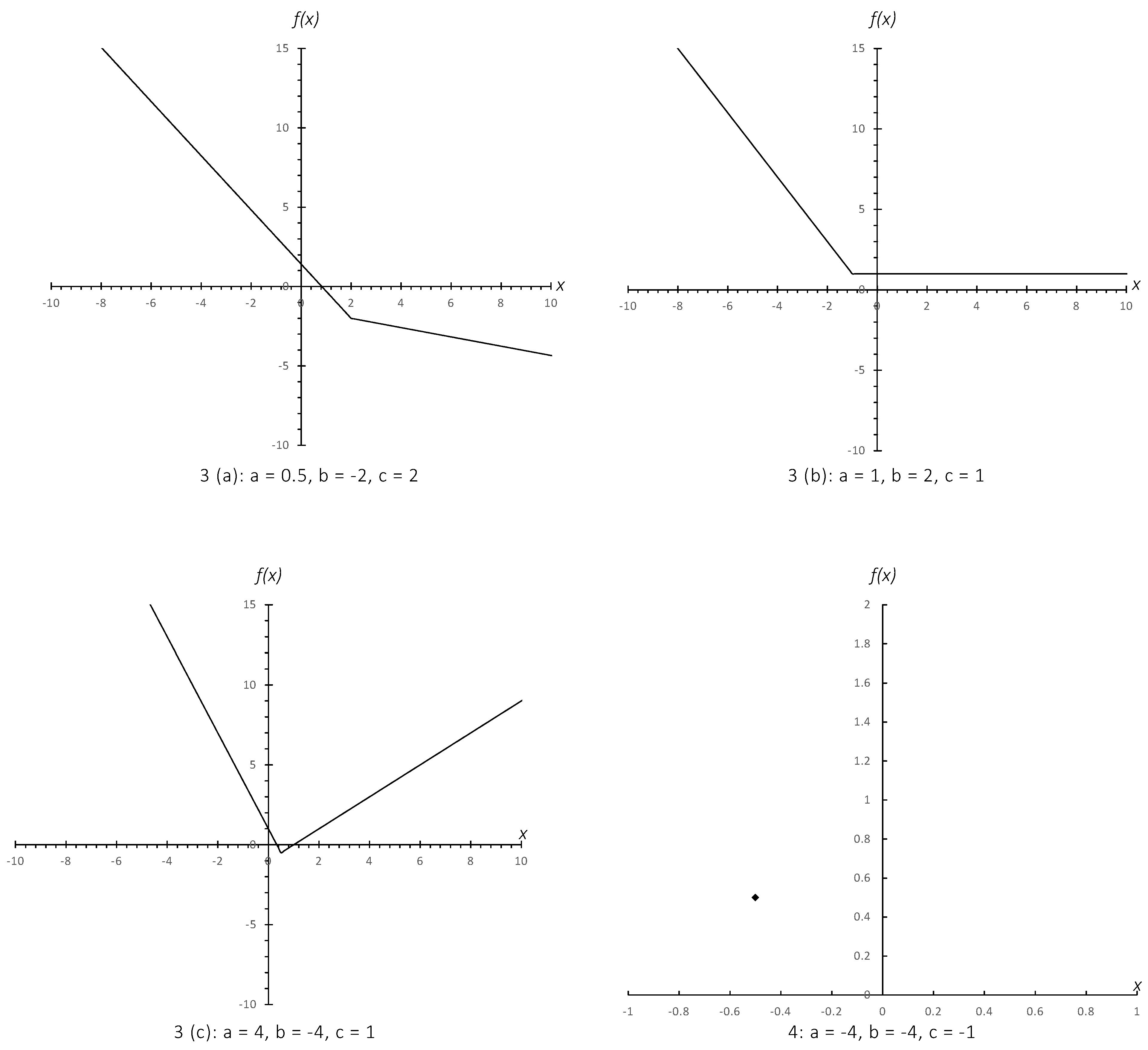
When $a\le 0$, $h(x_1,x_2)\ge 0$ and therefore Equation (8) is applicable. Then, the following is true for $f\left(x\right)$:

(a)

If $a<0$ and $b^2-4ac<0$, $f\left(x\right)\in \mathbb{C}$ for all x.

(b)

If $a<0$ and $b^2-4ac=0$, $f\left(x\right)$ consists of a single point at $x=-\frac{b}{2a}$; $f\left(x\right)\in \mathbb{C}$ elsewhere.

(c)

If $a<0$ and $b^2-4ac>0$, then $f\left(x\right)$ is concave between the roots of $g\left(x\right)$; $f\left(x\right)\in \mathbb{C}$ elsewhere.

(d)

If $a=0$, $f\left(x\right)$ is concave where $g\left(x\right)\ge 0$ and $f\left(x\right)\in \mathbb{C}$ elsewhere.

2.

When $a>0$ and $b^2-4ac>0$, $g\left(x\right)$ has two real roots and $f\left(x\right)\in \mathbb{C}$ between the roots. Therefore, we simply need to show that $h(x_1,x_2)\ge 0$ for $x_2\le x_1$ and $x_2\ge x_1$. $h(x_1,x_2)\ge 0$ for $x_2=x_1$. Without loss of generality, we fix $x_1$ at the smaller root. We will now show that $h(x_1,x_2)\ge 0$ for every $x_2<x_1$. Substituting the smaller root for $x_1$ in $h(x_1,x_2)$ results in:

$$\begin{array}{cc}\hfill h(x_1,x_2)& =2a{x}_2\left(\frac{-b-\sqrt{b^2-4ac}}{2a}\right)+b\left(\frac{-b-\sqrt{b^2-4ac}}{2a}\right)+b{x}_2+2c\hfill \\ \hfill & =\sqrt{b^2-4ac}\left(-x_2-\frac{b}{2a}\right)-\frac{b^2}{2a}+2c\hfill \end{array}$$

(10)

Because $x_2<x_1=\left(-\frac{b}{2a}-\frac{\sqrt{b^2-4ac}}{2a}\right)$, the following holds:

$$\begin{array}{c}\hfill h(x_1,x_2)>\sqrt{b^2-4ac}\left(\frac{b}{2a}+\frac{\sqrt{b^2-4ac}}{2a}-\frac{b}{2a}\right)-\frac{b^2}{2a}+2c=0\end{array}$$

(11)

Therefore, $h(x_1,x_2)\ge 0$ for $x_2<x_1$ and Equation (8) is applicable. Similarly, we can fix $x_1$ at the greater root and, using a similar process, we can prove that $h(x_1,x_2)\ge 0$ for $x_2>x_1$ and Equation (8) is again applicable. Consequently, when $a>0$ and $b^2-4ac>0$, $f\left(x\right)\in \mathbb{C}$ between the roots and concave outside of the roots.

3.

When $a>0$ and $b^2-4ac\le 0$, $g\left(x\right)$ has, at most, one real root and $f\left(x\right)\in \mathbb{R}$ for all x. When $b^2-4ac=0$, $x=-\frac{b}{2a}$ is the only root. Again, without loss of generality, we fix $x_1$ at this root. Substituting the root for $x_1$ in $h(x_1,x_2)$ results in:

$$\begin{array}{cc}\hfill h(x_1,x_2)& =2a{x}_2\left(-\frac{b}{2a}\right)-\frac{b^2}{2a}+b{x}_2+2c=-\frac{b^2}{2a}+2c\hfill \end{array}$$

(12)

Because $b^2\le 4ac$, the following holds:

$$\begin{array}{c}\hfill h(x_1,x_2)>-\frac{4ac}{2a}+2c=0\end{array}$$

(13)

Therefore, $h(x_1,x_2)\ge 0$ for $x_1\ne x_2$ and the simplification is valid, and thus, $f\left(x\right)$ is convex per Equation (8).

□

We observe that $g\left(x\right)$ having at most one real root is necessary for a unique interior solution that is finite valued, but not sufficient. The following lemma further establishes the sufficiency conditions.

Lemma 2.

Equation (5) has a unique interior minimum $\infty >x^{*}>0$ if and only if:

1.

$b^2-4ac\le 0$

2.

$a>1$

Proof. 

(1) is already established by Lemma 1. In order to prove (2), we will derive the closed-form euation for $x^{*}$. Let

$$\begin{array}{c}\hfill x_u=x^{*}+\Delta x\end{array}$$

(14)

$$\begin{array}{c}\hfill x_l=x^{*}-\Delta x\end{array}$$

(15)

for some $\Delta x>0$. Then, the following will hold for $x^{*}$ and $f\left(x\right)$:

$$\begin{array}{c}\hfill f\left(x_u\right)-f\left(x^{*}\right)\ge 0\end{array}$$

(16)

$$\begin{array}{c}\hfill f\left(x_l\right)-f\left(x^{*}\right)\ge 0\end{array}$$

(17)

Substituting Equation (5) into Equation (16), we obtain:

$$\begin{array}{c}\hfill \sqrt{a{x}_u^2+b{x}_u+c}-x_u-\sqrt{a{\left(x^{*}\right)}^2+b{x}^{*}+c}+x^{*}\ge 0\\ \hfill \sqrt{a{x}_u^2+b{x}_u+c}-\sqrt{a{\left(x^{*}\right)}^2+b{x}^{*}+c}-(x_u-x^{*})\ge 0\\ \hfill \frac{\sqrt{a{x}_u^2+b{x}_u+c}-\sqrt{a{\left(x^{*}\right)}^2+b{x}^{*}+c}}{(x_u-x^{*})}-1\ge 0\end{array}$$

Expanding the fraction by $\sqrt{a{x}_u^2+b{x}_u+c}+\sqrt{a{\left(x^{*}\right)}^2+b{x}^{*}+c}$ and simplifying, we obtain:

$$\begin{array}{c}\hfill \frac{a(x_u^2-{\left(x^{*}\right)}^2)+b(x_u-x^{*})}{(x_u-x^{*})(\sqrt{a{x}_u^2+b{x}_u+c}+\sqrt{a{\left(x^{*}\right)}^2+b{x}^{*}+c})}-1\ge 0\\ \hfill \frac{a(x_u+x^{*})+b}{\sqrt{a{x}_u^2+b{x}_u+c}+\sqrt{a{\left(x^{*}\right)}^2+b{x}^{*}+c}}\ge 1\end{array}$$

(18)

A similar analysis of Equation (17) will result in the following inequality:

$$\begin{array}{c}\hfill \frac{a(x_l+x^{*})+b}{\sqrt{a{x}_l^2+b{x}_l+c}+\sqrt{a{\left(x^{*}\right)}^2+b{x}^{*}+c}}\le 1\end{array}$$

(19)

Combining Equations (18) and (19), we obtain:

$$\begin{array}{cc}\hfill \frac{a(x_u+x^{*})+b}{\sqrt{a{x}_u^2+b{x}_u+c}+\sqrt{a{\left(x^{*}\right)}^2+b{x}^{*}+c}}\ge 1& \ge \frac{a(x_l+x^{*})+b}{\sqrt{a{x}_l^2+b{x}_l+c}+\sqrt{a{\left(x^{*}\right)}^2+b{x}^{*}+c}}\hfill \end{array}$$

(20)

Let $\Delta x$ become gradually smaller and approach zero. Then, both sides of Equation (20) will approach one another and therefore they will both approach 1 as well. It then follows that:

$$\begin{array}{c}\hfill \frac{2a{x}^{*}+b}{2\sqrt{a{\left(x^{*}\right)}^2+b{x}^{*}+c}}=1\end{array}$$

(21)

Note that Equation (21) is equivalent to

$$\begin{array}{c}\hfill f^{\prime }\left(x\right)=\frac{2a{x}^{*}+b}{2\sqrt{a{\left(x^{*}\right)}^2+b{x}^{*}+c}}-1=0\end{array}$$

(22)

However, we have not used knowledge of the derivative of any functional form to obtain this result. Equation (21) yields:

$$\begin{array}{c}\hfill 2a{x}^{*}+b=2\sqrt{a{\left(x^{*}\right)}^2+b{x}^{*}+c}\end{array}$$

(23)

We will now take the square of both sides to obtain a quadratic equation. Both negative and positive square roots of $\sqrt{a{\left(x^{*}\right)}^2+b{x}^{*}+c}$ satisfy the resulting Equation (24). Hence, we obtain two solutions, one that corresponds to a slope of 0 for $f\left(x\right)$, and another that corresponds to a slope of $-2$ for $f\left(x\right)$. The one that corresponds to zero slope is the interior minimum point and it is required to be positive. We know that $f\left(x\right)$ is required to be convex for a unique minimum, which means that its slope is negative to the left of the minimum point. Therefore, the larger of the two solutions of Equation (24) is the one that corresponds to the interior minimum point $x^{*}$. Taking the square of both sides and rearranging the terms, we obtain:

$$\begin{array}{c}\hfill 4(a-a^2){\left(x^{*}\right)}^2+4(b-ab)x^{*}+(4c-b^2)=0\end{array}$$

(24)

The discriminant of Equation (24) could be calculated as follows:

$$\begin{array}{cc}\hfill \Delta & ={\left[4(b-ab)\right]}^2-16(a-a^2)(4c-b^2)\hfill \\ \hfill & =16(1-a)(b^2-4ac)\hfill \end{array}$$

(25)

Then, the solution to Equation (24) will be the larger of the two roots:

$$\begin{array}{c}\hfill x^{*}=\frac{-4b(1-a)+4\sqrt{(1-a)(b^2-4ac)}}{2\left[4a\right(1-a\left)\right]}=\frac{1}{2a}\left[-b+\sqrt{\frac{b^2-4ac}{1-a}}\right]\end{array}$$

(26)

From (1), we know that $4ac\ge b^2$. Equation (26) requires $a>1$ in order to have a positive value inside the square root so that $x^{*}\in \mathbb{R}$, and it requires $a\ne 1$ to ensure that $x^{*}<\infty$. Therefore, we need $a>1$. It then follows that $c\ge 0$ because $4ac\ge b^2$ (this is not a separate condition, but a consequence of $a>1$ and $4ac\ge b^2$). □

We also need to establish conditions for $x^{*}>0$ and $f\left(x\right)>0$ because the underlying problem is the EPQ problem with backorders, where the problem is defined on $x>0$ and $f\left(x\right)>0$ for all $x>0$.

Lemma 3.

$f\left(x\right)>0$ for all $x\in \mathbb{R}$ if and only if $4(a-1)c>b^2$ and $a>1$.

Proof. 

The condition $f\left(x\right)>0$ can be simplified as follows:

$$\begin{array}{c}\hfill \sqrt{a{x}^2+bx+c}-x>0\Rightarrow a{x}^2+bx+c>x^2\Rightarrow (a-1)x^2+bx+c>0\end{array}$$

(27)

Equation (27) will be satisfied for all $x\in \mathbb{R}$ if and only if its graph entirely lies above the x axis—in other words, if it has no real roots and $a-1>0$ or $a>1$. Therefore, $\Delta =b^2-4(a-1)c<0$, or $4(a-1)c>b^2$. □

Lemma 4.

If $b\ge 0$, then $x^{*}>0$ if and only if $4c>b^2$.

Proof. 

If $b\ge 0$, $x^{*}>0$ requires:

$$\begin{array}{c}\hfill \sqrt{\frac{b^2-4ac}{1-a}}>b\Rightarrow \frac{b^2-4ac}{1-a}>b^2\Rightarrow 4c>b^2\end{array}$$

(28)

and if $b\le 0$, there is no additional condition for guaranteeing that $x^{*}>0$. □

We can now combine and summarize all of the necessary and sufficient conditions in the following theorem, as in Luo and Chou [31].

Theorem 1.

$f\left(x\right)$ is positive, convex, and has a unique positive finite valued non-boundary minimum if and only if $a>1$ and one of the following two conditions is satisfied:

1.

$b<0$ and $4(a-1)c>b^2$

2.

$b\ge 0$ and $4c>b^2$

Proof. 

Immediate from Lemmas 1–4: if $a>1$, then $4ac>4(a-1)c>b^2$ as well as $4ac>4c>b^2$, which means, for case 1, we can drop $b^2-4ac\le 0$ and keep $4(a-1)c>b^2$; and for case 2, we can drop $b^2-4ac\le 0$ and keep $4c>b^2$ □

4. The Original Inventory Problem

In the original EPQ with the backordering problem of Equation (4), $a=1+\alpha$; $b=0$, and $c=\beta$. Clearly, $a=1+\frac{b}{h}>1$; therefore, the only remaining requirement is $4\beta >0$ and this is also satisfied because $\beta =\frac{2\rho KD}{h}>0$. Therefore, we can substitute these values of a, b, and c in Equation (26) and obtain the optimal solution:

$$\begin{array}{c}\hfill B^{*}=\sqrt{\frac{\beta }{\alpha (1+\alpha )}},\mathrm{and}f\left(B^{*}\right)=\alpha B\end{array}$$

(29)

Contrary to the approach of Luo and Chou [31], our approach can directly be applied to Equation (4) as well. Let $B^{*}$ be the minimum point of $f\left(B\right)$ that is not a boundary solution and let

$$\begin{array}{c}\hfill B_u=B^{*}+\Delta B\end{array}$$

(30)

$$\begin{array}{c}\hfill B_l=B^{*}-\Delta B\end{array}$$

(31)

for some $\Delta B>0$. Then, the following will hold due to $B^{*}$ being a non-boundary minimum point:

$$\begin{array}{c}\hfill f\left(B_u\right)-f\left(B^{*}\right)\ge 0\end{array}$$

(32)

$$\begin{array}{c}\hfill f\left(B_l\right)-f\left(B^{*}\right)\ge 0\end{array}$$

(33)

Equation (32) can further be simplified as follows:

$$\begin{array}{c}\hfill \sqrt{(1+\alpha )B_u^2+\beta }-B_u-\sqrt{(1+\alpha ){\left(B^{*}\right)}^2+\beta }+B^{*}\ge 0\\ \hfill \frac{\sqrt{(1+\alpha )B_u^2+\beta }-\sqrt{(1+\alpha ){\left(B^{*}\right)}^2+\beta }}{B_u-B^{*}}-1\ge 0\end{array}$$

Expanding the fraction by $\sqrt{(1+\alpha )B_u^2+\beta }+\sqrt{(1+\alpha ){\left(B^{*}\right)}^2+\beta }$ results in

$$\begin{array}{c}\hfill \frac{(1+\alpha )(B_u^2-{\left(B^{*}\right)}^2)}{(B_u-B^{*})(\sqrt{(1+\alpha )B_u^2+\beta }+\sqrt{(1+\alpha ){\left(B^{*}\right)}^2+\beta })}-1\ge 0\\ \hfill \frac{(1+\alpha )(B_u+B^{*})}{\sqrt{(1+\alpha )B_u^2+\beta }+\sqrt{(1+\alpha ){\left(B^{*}\right)}^2+\beta }}\ge 1\end{array}$$

(34)

Applying the same approach to Equation (33) will result in:

$$\begin{array}{c}\hfill \frac{(1+\alpha )(B_l+B^{*})}{\sqrt{(1+\alpha )B_l^2+\beta }+\sqrt{(1+\alpha ){\left(B^{*}\right)}^2+\beta }}\le 1\end{array}$$

(35)

Again, combining Equations (34) and (35), we obtain:

$$\begin{array}{c}\hfill \frac{(1+\alpha )(B_u+B^{*})}{\sqrt{(1+\alpha )B_u^2+\beta }+\sqrt{(1+\alpha ){\left(B^{*}\right)}^2+\beta }}\ge 1\ge \frac{(1+\alpha )(B_l+B^{*})}{\sqrt{(1+\alpha )B_l^2+\beta }+\sqrt{(1+\alpha ){\left(B^{*}\right)}^2+\beta }}\end{array}$$

(36)

Let $\Delta B$ become gradually smaller and approach zero. Then, both sides of Equation (36) will approach one another and therefore they will both approach 1 as well. It then follows that:

$$\begin{array}{cc}\hfill & \frac{2(1+\alpha )B^{*}}{2\sqrt{(1+\alpha ){\left(B^{*}\right)}^2+\beta }}=1\hfill \end{array}$$

(37)

Therefore, the solution to Equation (37) is:

$$\begin{array}{c}\hfill B^{*}=\sqrt{\frac{\beta }{\alpha (1+\alpha )}}\end{array}$$

(38)

$f\left(B\right)$ is strictly convex if and only if the following holds for $B_1$, $B_2\in \mathbb{R}$, $B_1\ne B_2$ and $0<\lambda <1$:

$$\begin{array}{c}\hfill \lambda f\left(B_1\right)+(1-\lambda )f\left(B_2\right)>f(\lambda B_1+(1-\lambda )B_2)\end{array}$$

(39)

Equation (39) can be simplified further as follows:

$$\begin{array}{cc}\hfill & \lambda \sqrt{(1+\alpha )B_1^2+\beta }-\lambda B_1+(1-\lambda )\sqrt{(1+\alpha )B_2^2+\beta }-(1-\lambda )B_2>\hfill \\ \hfill & \sqrt{(1+\alpha ){(\lambda B_1+(1-\lambda )B_2)}^2+\beta }-\lambda B_1-(1-\lambda )B_2\hfill \\ \hfill & -2\lambda (1-\lambda )\beta +2\lambda (1-\lambda )\sqrt{[(1+\alpha )B_1^2+\beta ][(1+\alpha )B_2^2+\beta ]}>\hfill \\ \hfill & 2\lambda (1-\lambda )(1+\alpha )B_1{B}_2\hfill \end{array}$$

(40)

Dividing both sides by the positive term $2\lambda (1-\lambda )$, we obtain:

$$\begin{array}{cc}\hfill & \sqrt{[(1+\alpha )B_1^2+\beta ][(1+\alpha )B_2^2+\beta ]}>(1+\alpha )B_1{B}_2+\beta \hfill \\ \hfill & (1+\alpha )\beta (B_1^2+B_2^2-2B_1{B}_2)>0\Rightarrow {(B_1-B_2)}^2>0\hfill \end{array}$$

Therefore, $B^{*}>0$ is a unique non-boundary finite valued optimal solution that also satisfies $f\left(B^{*}\right)>0$.

5. Limitations and Further Research

The proposed method does not explicitly use the derivative of any function and, instead, derives the optimal solution using only algebraic manipulations. It is simple, succinct, and intuitive, which makes it a useful pedagogical tool to teach inventory models to students with limited skills in differential calculus. On the other hand, it implicitly uses the first derivative of the total cost function, by obtaining it through algebraic operations, as shown in Çalışkan [33]. It implicitly assumes that the total cost function is continuous and continuously differentiable. When this is not the case, it will require further steps and will become more complicated. However, the same is true for any other approach when the total cost function is not continuous. Further research may apply the proposed method to total cost functions that are not continuous, and to other problems in inventory management and operations research. It may also be adapted to situations in which there are constraints and/or more decision variables in the problem.

6. Conclusions

In this paper, we answer the open question posed in Chang et al. [7]: deriving the optimal solution for a reformulation of the EPQ problem with backorders using an approach that does not require derivatives. The earlier approach proposed by Luo and Chou [31] is not entirely correct and complete, as shown in Çalışkan [32], so the open question is still outstanding. We also point out that the approach in Luo and Chou [31] is far too complicated that it defeats the purpose, which is simplifying the optimization by not using differential calculus so that undergraduate or even high school students, or practitioners without a working knowledge of differential calculus, can understand it. Our approach, on the other hand, is simple, succinct, and easy to follow. We consider the generalized version of the open question proposed by Lau et al. [29] and derive the necessary and sufficient conditions for the problem to have an acceptable optimal solution for the underlying EPQ problem, as well as the optimal solution itself. We also show that our approach could be applied directly to the original inventory problem with ease. Finally, we study the general problem to provide more insights and show that it can assume different characteristics depending on its parameters (Appendix A).

References

- Harris, F. How Many Parts to Make At Once. Fact. Mag. Manag. 1913, 10, 135ߝ136, 152. [Google Scholar] [CrossRef]
- Grubbström, R.W.; Erdem, A. The EOQ with backlogging derived without derivatives. Int. J. Prod. Econ. 1999, 59, 529–530. [Google Scholar] [CrossRef]
- Cárdenas-Barrón, L.E. The economic production quantity (EPQ) with shortage derived algebraically. Int. J. Prod. Econ. 2001, 70, 289–292. [Google Scholar] [CrossRef]
- Wee, H.; Chung, S.; Yang, P. Technical Note A Modified EOQ Model with Temporary Sale Price Derived without Derivatives. Eng. Econ. 2003, 48, 190–195. [Google Scholar] [CrossRef]
- Huang, Y.F. The deterministic inventory models with shortage and defective items derived without derivatives. J. Stat. Manag. Syst. 2003, 6, 171–180. [Google Scholar] [CrossRef]
- Ronald, R.; Yang, G.K.; Chu, P. Technical note: The EOQ and EPQ models with shortages derived without derivatives. Int. J. Prod. Econ. 2004, 92, 197–200. [Google Scholar] [CrossRef]
- Chang, S.J.; Chuang, J.P.; Chen, H.J. Short comments on technical note—The EOQ and EPQ models with shortages derived without derivatives. Int. J. Prod. Econ. 2005, 97, 241–243. [Google Scholar] [CrossRef]
- Sphicas, G.P. EOQ and EPQ with linear and fixed backorder costs: Two cases identified and models analyzed without calculus. Int. J. Prod. Econ. 2006, 100, 59–64. [Google Scholar] [CrossRef]
- Omar, M.; Zubir, M.B.; Moin, N. An alternative approach to analyze economic ordering quantity and economic production quantity inventory problems using the completing the square method. Comput. Ind. Eng. 2010, 59, 362–364. [Google Scholar] [CrossRef]
- Cárdenas-Barrón, L.E. Optimal manufacturing batch size with rework in a single-stage production system–-A simple derivation. Comput. Ind. Eng. 2008, 55, 758–765. [Google Scholar] [CrossRef]
- Wee, H.M.; Chung, C.J. A note on the economic lot size of the integrated vendor–-Buyer inventory system derived without derivatives. Eur. J. Oper. Res. 2007, 177, 1289–1293. [Google Scholar] [CrossRef]
- Chung, K.J. “A note on the economic lot size of the integrated vendor–-buyer inventory system derived without derivatives”: A comment. Eur. J. Oper. Res. 2009, 198, 979–982. [Google Scholar] [CrossRef]
- Teng, J.T. A simple method to compute economic order quantities. Eur. J. Oper. Res. 2009, 198, 351–353. [Google Scholar] [CrossRef]
- Leung, K.N.F. Some comments on “A simple method to compute economic order quantities”. Eur. J. Oper. Res. 2010, 201, 960–961. [Google Scholar] [CrossRef]
- Cárdenas-Barrón, L.E. A simple method to compute economic order quantities: Some observations. Appl. Math. Model. 2010, 34, 1684–1688. [Google Scholar] [CrossRef][Green Version]
- Cárdenas-Barrón, L.E. An easy method to derive EOQ and EPQ inventory models with backorders. Comput. Math. Appl. 2010, 59, 948–952. [Google Scholar] [CrossRef]
- Ouyang, L.Y.; Chang, C.T.; Shum, P. The EOQ with defective items and partially permissible delay in payments linked to order quantity derived algebraically. Cent. Eur. J. Oper. Res. 2012, 20, 141–160. [Google Scholar] [CrossRef]
- Cárdenas-Barrón, L.E.; Wee, H.M.; Blos, M.F. Solving the vendor–-Buyer integrated inventory system with arithmetic–-Geometric inequality. Math. Comput. Model. 2011, 53, 991–997. [Google Scholar] [CrossRef]
- Cárdenas-Barrón, L.E. The derivation of EOQ/EPQ inventory models with two backorders costs using analytic geometry and algebra. Appl. Math. Model. 2011, 35, 2394–2407. [Google Scholar] [CrossRef]
- Lin, S.S.C. Note on “The derivation of EOQ/EPQ inventory models with two backorders costs using analytic geometry and algebra”. Appl. Math. Model. 2019, 73, 378–386. [Google Scholar] [CrossRef]
- Teng, J.T.; Cárdenas-Barrón, L.E.; Lou, K.R. The economic lot size of the integrated vendor–-buyer inventory system derived without derivatives: A simple derivation. Appl. Math. Comput. 2011, 217, 5972–5977. [Google Scholar] [CrossRef]
- Sphicas, G.P. Generalized EOQ formula using a new parameter: Coefficient of backorder attractiveness. Int. J. Prod. Econ. 2014, 155, 143–147. [Google Scholar] [CrossRef]
- Luo, X.R. A Detailed Examination of Sphicas (2014), Generalized EOQ Formula Using a New Parameter: Coefficient of Backorder Attractiveness. Int. J. Prod. Econ. 2019, 11, 931. [Google Scholar] [CrossRef]
- Minner, S. A note on how to compute economic order quantities without derivatives by cost comparisons. Int. J. Prod. Econ. 2007, 105, 293–296. [Google Scholar] [CrossRef]
- Wee, H.M.; Wang, W.T.; Chung, C.J. A modified method to compute economic order quantities without derivatives by cost-difference comparisons. Eur. J. Oper. Res. 2009, 194, 336–338. [Google Scholar] [CrossRef]
- Cárdenas-Barrón, L. A note on how to compute economic order quantities without derivatives by cost comparisons: Some comments. Int. J. Appl. Manag. Sci. 2010, 2, 198–204. [Google Scholar] [CrossRef]
- Chung, C.J. An easy method to derive the integrated vendor—Buyer production—Inventory model with backordering using cost–difference rate comparison approach. Math. Comput. Model. 2013, 57, 632–640. [Google Scholar] [CrossRef]
- Widyadana, G.A.; Cárdenas-Barrón, L.E.; Wee, H.M. Economic order quantity model for deteriorating items with planned backorder level. Math. Comput. Model. 2011, 54, 1569–1575. [Google Scholar] [CrossRef]
- Lau, C.; Chou, E.; Dementia, J. Criterion to ensure uniqueness for minimum solution by algebraic method for inventory model. Int. J. Eng. Appl. Sci. 2016, 3, 71–73. [Google Scholar]
- Chiu, C.; Li, Y.; Julian, P. Improvement for Criterion for Minimum Solution of Inventory Model with Algebraic Approach. J. Bus. Manag. 2017, 19, 73–78. [Google Scholar] [CrossRef]
- Luo, X.R.; Chou, C.S. Technical note: Solving inventory models by algebraic method. Int. J. Prod. Econ. 2018, 200, 130–133. [Google Scholar] [CrossRef]
- Çalışkan, C. On “Technical note: Solving inventory models by algebraic method”. J. Stat. Manag. Syst. 2021, 24, 1533–1541. [Google Scholar] [CrossRef]
- Çalışkan, C. A general approach for the derivation of optimal solutions without derivatives. Int. J. Syst. Sci. Oper. Logist. 2021, 1–12. [Google Scholar] [CrossRef]
- Jensen, J.L.W.V. Sur les fonctions convexes et les inégalités entre les valeurs moyennes. Acta Math. 1906, 30, 175–193. [Google Scholar] [CrossRef]
Publisher’s Note: MDPI stays neutral with regard to jurisdictional claims in published maps and institutional affiliations. |
© 2022 by the author. Licensee MDPI, Basel, Switzerland. This article is an open access article distributed under the terms and conditions of the Creative Commons Attribution (CC BY) license (https://creativecommons.org/licenses/by/4.0/).