Position Estimation Method for a Fluorescently Labeled Tumor Based on Beer’s Law: An Analysis Using Monte Carlo Simulations

Abstract

Estimating the depth of a fluorescently labeled tumor is beneficial in tumor resection. In this study, we proposed a method for the three-dimensional position estimation of fluorescent tumors using Monte Carlo simulations. A limited proof-of-concept experiment was conducted, and the two-dimensional position of a tumor was estimated by calculating the centroid of the fluorescence distribution, which was obtained by using excitation light to scan the surface of the model. The depth of the tumor was estimated by fitting the analytical equation based on Beer’s law to the diffuse fluorescence profile on the surface of the model. In the estimation of the two-dimensional position, the distance between the embedded and estimated tumor coordinates was 0.71 mm. The estimated tumor depths of 2–6 mm closely matched the embedded depths, with an error rate of approximately 20%. In previous studies, depth estimation was limited to 1–5 mm using visible light, whereas for the simulation used in the present study, the use of longer wavelengths enabled estimation at slightly greater depths.

1. Introduction

Detection techniques used for fluorescent objects in tissues using non-targeted and targeted tracers have made remarkable progress in medical applications. Non-targeted tracers such as fluorescein in the visible region (VIS) visualize retinal perfusion, and indocyanine green (ICG) in the near-infrared region (NIR) emits strong fluorescence within the body because it accumulates in tumors with high metabolic efficiency [1,2]. Targeted tracers are composed of a carrier molecule (such as an antibody, a peptide, or a small molecule) with a fluorescent probe and are specifically accumulated for the target [3]. In previous studies, tracers were employed for the detection of breast tumors, the identification of lymph node metastasis resulting from said tumors, or tumor resection in neurosurgery [4,5]. Since tumor depth estimation is beneficial for resection, fluorescence molecular tomography was developed to estimate the three-dimensional localization of fluorescent objects in tissues [6]. However, data acquisition is time-consuming, the required equipment is expensive, and the optical system is very sensitive to small misalignments in the instrument [7]. As a result, improved estimation methods for tumor depth have been proposed.

Tumor depth was estimated by measuring the ratio of the fluorescence at two wavelengths of 670 and 720 nm in combination with normalization techniques based on diffuse reflectance measurements [7]. The wavelength pair was limited due to the smaller spectroscopic changes in hemoglobin absorption above 700 nm. Fluorescence topography was determined up to a 5 mm depth with millimeter-depth accuracy in turbid media with optical properties representative of normal brain tissue. Petusseau et al. developed a depth-sensing imaging technique using light detection and ranging time-of-flight technology to determine the depth of the target tissue [8]. Because fluorescence wavelengths with IRDye680 were limited due to specifications of the single-photon avalanche diode sensor, estimating the depth with a sub mm resolution up to a maximum of 5 mm was possible. Thus, efforts to improve the evaluated depth are needed, which can be achieved by extending the fluorescence wavelength. Dang et al. proposed a deep-tissue optical imaging technique in 1000–1700 nm using rare-earth-doped probes, where the surface area of a tissue with an embedded fluorescent object was excited by a laser of 980 nm in the trans-illumination scanning configuration [9]. Fluorescent objects with different emission wavelengths were differentiated using hyperspectral imaging, and each depth up to 50 mm was estimated using hyper-diffuse imaging.

In the present study, fluorescence obtained by the diffuse reflectance measurement was evaluated using the hyper diffuse imaging method, and the feasibility of the depth estimation was examined using Monte Carlo simulations with ICG (approved for clinical use), which is excited by and emitted at wavelengths of 785 nm and 820 nm, respectively. Based on previous studies [10,11,12,13,14], we set the appropriate optical parameters of the absorption coefficient, scattering coefficient, refractive index, and anisotropy for a homogeneous tissue phantom with 50 × 50 × 28 mm, and a fluorescent sphere tumor with a 4 mm diameter was embedded at different depths of 1 to 6 mm. In the simulation, incident photons were excluded from fluorescence using a dichroic mirror and a long-pass filter. When a two-dimensional scan was performed at a constant excitation light intensity, fluorescence fluence maps on the phantom surface were obtained for each excitation light irradiation position, and the centroid coordinate was calculated from the fluorescence intensity ratios at four excitation positions. For the depth estimation of the fluorescent object, the excitation light intensity irradiated on the surface coordinate was adjusted based on the sensitivity in the near-infrared region of the actual camera. The obtained fluorescence fluence map was converted into a diffuse fluorescence profile, and an analytical equation derived from Beer’s law was fitted to the results for tumor depth estimation. Although the estimated depth at 1 mm had a 93% error, the depth between 2 and 6 mm indicated high accuracy compared to a previous study [7]. In addition, we conducted a limited proof-of-concept experiment based on simulations.

2. Materials and Methods

2.1. Model Setup

Figure 1 shows a scheme of the model used in this study. A voxel-based model with dimensions of 500 × 500 × 280 pixels (50 × 50 × 28 mm) was created [15], in which a scattering medium was defined. Appropriate optical properties, including the scattering coefficient (${\mu }_s$), absorption coefficient (${\mu }_a$), anisotropy factor ($g$), and refractive index ($n$), were assigned to each voxel, as listed in Table 1 [10,11,12,13,14]. The scattering medium was assumed to contain a 1% intralipid solution, which is commonly used to mimic the scattering characteristics of a biological tissue [16]. A fluorescent tumor with a diameter of 4 mm, reported as the initial tumor size in Weng et al.’s study, was used in this model [17]. The tumor shape was assumed to be spherical because it is difficult to simulate complex geometries resembling actual tumors. The fluorescent tumor was embedded at depths ranging from 1 to 6 mm from the top surface of the scattering medium, with coordinates of x = 250 and y = 250 in the XY plane. ICG (Ex 785 nm/Em 820 nm, QY 0.09, C 20 µM, εC: 3.4 cm⁻¹), the only near-infrared fluorescent dye approved by the FDA, was assumed to be used as a fluorescent dye [10,18]. This study assumes that the fluorescent dye concentration within the tumor is constant, which several previous studies have done to simplify the analysis of light propagation [19,20].

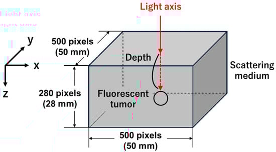
Figure 1. Scheme of the simulation model. A fluorescent tumor is embedded at a defined depth within a three-dimensional voxel-based model (500 × 500 × 280 pixels) representing a scattering medium. The excitation light is incident perpendicular from the top surface along the light axis, indicated by the red arrow. The coordinate system is defined so that the X-axis corresponds to the horizontal direction, the Y-axis to the vertical direction, and the Z-axis to the depth direction.

Table 1. Optical properties of the simulation model.

Wavelength (nm)	Layer	${\mathit{\mu }}_{\mathit{a}}$ $[{\mathbf{c}\mathbf{m}}^{-1}$]	${\mathit{\mu }}_{\mathit{s}}$ $[{\mathbf{c}\mathbf{m}}^{-1}$]	n	g
785	Medium	0.018	30	1.33	0.67
	Tumor	1	150	1.45	0.9
820	Medium	0.03	27.4	1.33	0.67
	Tumor	0.7	140	1.45	0.9

2.2. Monte Carlo Simulation

For the Monte Carlo simulation, photon migration through the tissue was calculated using Wang et al.’s computational procedure [21]. The simulation code was developed by Iida et al. [10] using the C programming language within Microsoft Visual Studio 2022 (Version 17.1.4). Briefly, the travel distance and direction of the photon were determined using random numbers generated by the Mersenne twister method [22]. The weight of each excitation photon was initially unity and then subsequently reduced by ${\mu }_a/{\mu }_t$ (${\mu }_t$ is the sum of ${\mu }_s$ and ${\mu }_a$) during one movement of the photon to the next site. At each boundary between the two layers, the photons were reflected or transmitted based on the Fresnel reflectance, which was calculated from the refractive indices $n$ of each layer [21]. Random photon paths were calculated until the weight of the photon was reduced to below the threshold or left the medium. The weight of each photon absorbed within each voxel was scored for fluorescence after inputting a million excitation photons, and the sum of all photon weights in each voxel was divided by the ${\mu }_a$ of the voxel to obtain the fluence. If the input photon beam is measured in W/cm² as the power density, the unit of fluence is also W/cm² [21]. In the present study, the fluence in each voxel was multiplied by the particular irradiation intensity (W/cm²) and divided by the number of excitation photons to obtain the absorbed fluence per voxel (W/cm²).

2.3. Monte Carlo Fluorescence Model

In this study, one million photons were launched from the XY plane (see Figure 1), and each photon was tracked during random walks based on the optical parameters of the tissues (Table 1). Excitation photon propagation was displayed as the internal photon distribution using fluence, which scores the photon weight absorbed within the grid elements (r, z) based on the absorption coefficients of the scattering medium and the fluorescent tumor. Because the step size was 0.01 cm, each element occupied ${0.01}^3$ ${\mathrm{c}\mathrm{m}}^3$ [23]. In the present study, fluence was considered to be the weight of the photons that passed per unit area; in other words, it is the amount of energy that is passed per unit area ($\mathrm{W}/{\mathrm{c}\mathrm{m}}^2$). After completion of the tracking of all excitation photons, a million photons at the emission wavelength were generated at randomly determined points within the tumor. The initial weight of a fluorescence photon was calculated as the excitation photon weight multiplied by the quantum yield (QY) of the fluorescent dye. In the first generation step, both azimuth and zenith angles toward the subsequent interaction site were set to isotropic using different random numbers. Thereafter, the isotropic azimuth and zenith angles with substantial forward-scattering properties toward the next interaction site were generated.. The fluorescence intensity (W/cm²) was calculated by multiplying the fluence at each voxel by a specified irradiation intensity (W/cm²) and dividing by the number of excitation photons [23].

2.4. Three-Dimensional Position Estimation (Simulation Methods)

2.4.1. Two-Dimensional Position Estimation (Simulation Methods)

To estimate the two-dimensional position of the fluorescent tumor, the excitation light was scanned on the top surface of the model. In the present study, the excitation light scanning range and interval were set considering the balance between simulation accuracy and computation time. Excitation light was irradiated at 25 points with 5 mm intervals over a 20 × 20 mm area on the top surface of the model. For each excitation light irradiation position, a fluorescence fluence map on the model surface was generated, and the accuracy of the two-dimensional position estimation was subsequently evaluated. Therefore, the distance between the estimated fluorescent tumor coordinates and the actual embedded tumor coordinates was calculated, where the estimated coordinates—defined as the centroid of the fluorescence intensity ratios obtained at the four points on the model surface—were calculated using the results from four of the twenty-five simulated excitation light irradiation positions. The fluorescence intensity represents the average value within a 10 × 10-pixel area centered at the centroid coordinates of each fluence map. The centroid ($x_c$, $y_c$) was calculated using Equation (1).

$$x_c={\displaystyle \frac{{\sum }_{i=1}^N{I}_i{x}_i}{{\sum }_{i=1}^N{I}_i}}{y}_c={\displaystyle \frac{{\sum }_{i=1}^N{I}_i{y}_i}{{\sum }_{i=1}^N{I}_i}}.$$

(1)

In this equation, ($x_c$, $y_c$), $N$, $(x,y)$, and $I$ are the centroid coordinates, the number of data points, the excitation light irradiation coordinates, and the fluorescence intensity, respectively. Then, the distance between the centroid $(x_c,y_c)$ and the embedded fluorescent tumor center $(250,250)$ was calculated. Moreover, to simulate the excitation light scanning expected in the actual measurements, we performed simulations using a 1 mm scanning interval to determine how fluorescence fluence changes based on the distance between the excitation position and the tumor. As a result of these conditions, the excitation light scanning assumed in the experimental measurements was reproduced, enabling an evaluation of how the fluorescence fluence obtained on the surface of the scattering medium varies with the distance between the fluorescent tumor and the excitation light irradiation position. The excitation light intensity was set to 0.5 $\mathrm{m}\mathrm{W}$/${\mathrm{c}\mathrm{m}}^2$ at all depths for the purpose of estimating the two-dimensional position of the tumor. This value was selected based on the maximum excitation intensity experimentally determined with the camera (MCM-303NIR, Gazoo, Niigata, Japan) and did not cause fluorescence saturation at a depth of 1 mm. The excitation beam diameter was set to 1 mm, which corresponded to the minimum beam size of the light source used for the actual measurement system.

2.4.2. Depth Estimation (Simulation Methods)

To estimate the depth of the fluorescent tumor, simulations were performed for tumor depths ranging from 1 to 6 mm. Fluorescence becomes more strongly scattered as the tumor depth increases, which is a characteristic that was used to estimate the tumor depth in this study. Therefore, for each tumor depth ranging from 1 to 6 mm, the excitation light intensity was set to the maximum value that did not exceed the saturation intensity of the camera used in the experimental system. This is based on the fact that, in actual measurements, it is easy to adjust the excitation light output while monitoring the camera image in real time to ensure that the fluorescence intensity is similar at each depth. Based on the fluorescence imaging results obtained with the experimental system, simulations were conducted to determine the fluorescence fluence that did not exceed the camera’s saturation intensity. As a result, the fluorescence fluence at each depth was 1.29 × 10⁻⁵, and multiple simulations were subsequently performed to determine the excitation light intensity for each fluorescent tumor depth, resulting in excitation intensities for tumor depths of 1–6 mm being 0.5, 1.0, 2.3, 4.5, 7.0, and 14.5 $\mathrm{m}\mathrm{W}/{\mathrm{c}\mathrm{m}}^2$, respectively. Based on a previous study [9], the resulting fluorescence fluence maps for each depth were converted into diffuse fluorescence profiles, and the analytical equation was fitted to these profiles. We used fluorescence fluence maps at the surface of the scattering medium obtained for each tumor depth. The map was converted into a diffuse fluorescence profile representing the change in fluorescence fluence with distance from the excitation light irradiation position. The estimated tumor depth was obtained by fitting the following analytical Equation (2)—which describes the change in fluorescence intensity as a function of the distance—to this profile.

$$I\left(r\right)=A·e^{-{\mu }_{\mathrm{e}\mathrm{f}\mathrm{f}}(d+\sqrt{r^2+d^2})}.$$

(2)

In this equation, $I\left(r\right)$, $A$, ${\mu }_{\mathrm{e}\mathrm{f}\mathrm{f}}$, $d$, and $r$ are fluorescence fluence as a function of the distance $r$, an arbitrary constant, the attenuation coefficient of the scattering medium, the depth of the fluorescent tumor, and the distance from the excitation position, respectively. Fitting parameters included $A$, ${\mu }_{\mathrm{e}\mathrm{f}\mathrm{f}}$, and $d$, and fitting was performed using a nonlinear least-squares method, applying an initial value of 0.80 only to ${\mu }_{\mathrm{e}\mathrm{f}\mathrm{f}}$, whereas no initial values were assigned to $A$ and $d$. The attenuation coefficient of the scattering medium was calculated using Equation (2) below.

$${\mu }_{\mathrm{e}\mathrm{f}\mathrm{f}}=\sqrt{3·{\mu }_{\mathrm{a}}({\mu }_{\mathrm{a}}+{\mu }_{\mathrm{s}}^{\prime })}.$$

(3)

Here, ${\mu }_{\mathrm{e}\mathrm{f}\mathrm{f}}$, ${\mu }_{\mathrm{a}}$, and ${\mu }_{\mathrm{s}}^{\prime }$ are the attenuation coefficients of the scattering medium, the absorption coefficient of the medium, and the reduced scattering coefficient [9] of the medium, respectively. In Table 1, the attenuation coefficient of the medium at two wavelengths, 785 nm and 820 nm, was calculated using the absorption coefficient (${\mu }_{\mathrm{a}}$), scattering coefficient (${\mu }_{\mathrm{s}}$), and anisotropy parameter ($g$). As a result, ${\mu }_{\mathrm{e}\mathrm{f}\mathrm{f}}$ was determined to be 0.73 and 0.90 at the excitation and fluorescence wavelengths, respectively. Considering the attenuation of both excitation and fluorescence light, the initial value of the attenuation coefficient was set to 0.80. The analyses described in this section were conducted using MATLAB R2021a, except for the curve fitting process, which was performed using the Solver function in Microsoft Excel.

2.5. Limited Proof-of-Concept Experiment (Experimental Methods)

2.5.1. System Setup

A limited proof-of-concept experiment was conducted using the system shown in Figure 2. The 785 nm excitation light source (LP785-SF20, THORLABS, Newton, NJ, USA) was connected to a two-axis motorized stage (HPS120-60X-M5, SIGMAKOKI Co., Tokyo, Japan), which was connected to a controller (SHOT-702H, SIGMAKOKI Co., Tokyo, Japan) and a PC, and was operated using a PC program. The excitation light was scanned over a 20 × 20 mm area on the sample surface at 1 mm intervals, passed through a dichroic mirror (69220, Edmund Optics, Barrington, NJ, USA) placed at 45°, and scanned over the sample containing the fluorescent dye. The fluorescence emitted upward was reflected by the dichroic mirror and detected by the camera (MCM-303NIR, Gazoo Co., Niigata, Japan), which has a quantum efficiency of 40% around 800 nm, and the acquired images were 785 × 480 pixels (55 × 35 mm). These images are represented in 8-bit grayscale. The sample to be imaged consisted of a 50 × 50 × 50 mm container, a 1% intralipid solution (Intralipos 20%, Otsuka Pharmaceutical Co., Tokyo, Japan), a fluorescent dye, and a supporting pillar. ICG (I0535, Tokyo Chemical Industry, Tokyo, Japan) was used as a 4 mm diameter spherical fluorophore, which was fabricated by pouring an agar solution mixed with ICG (20 µM) into a silicone mold with a 4 mm diameter spherical cavity and allowing it to solidify. By mounting the fluorophore on a supporting pillar with a height of 19–23 mm and filling the container with intralipid solution up to a height of 28 mm, fluorophore depths of 1–5 mm were achieved.

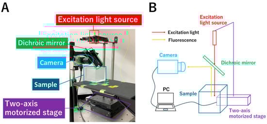
Figure 2. System for the limited proof-of-concept experiment (A) and its schematic diagram (B). The 785 nm excitation light source is connected to a two-axis motorized stage, which is connected to a controller and a PC, and was operated using a PC program. The excitation light passes through a dichroic mirror placed at 45° and is used to scan the sample containing the fluorophore. The fluorescence emitted upward is reflected by the dichroic mirror and detected by the camera.

2.5.2. Two-Dimensional Position Estimation (Experimental Methods)

To estimate the two-dimensional position of the fluorophore, the excitation light was scanned over a 20 × 20 mm area on the top surface of the sample at 1 mm intervals, and an image was acquired at each excitation light irradiation position. In the simulation, the accuracy of two-dimensional position estimation was evaluated using fluence maps obtained at four excitation positions, each located 5 mm away from the fluorophore. Because the scanning interval was 1 mm, the accuracy of two-dimensional position estimation was evaluated using the images acquired at four excitation positions embedded 1–5 mm from the fluorophore at 1 mm increments for each depth. For each depth from 1 to 5 mm, three experiments were performed.

2.5.3. Depth Estimation ( Experimental Methods)

To estimate the depth of the fluorophore, the excitation light intensity was adjusted at each depth from 1 to 5 mm so that the fluorescence intensity reached the maximum level without saturation. The excitation light intensities at depths of 1–5 mm were 0.2, 1.9, 4.2, 8.4, and 15.0 mW, respectively. Because the maximum output of the excitation light source in the experimental system was 20 mW, the experiment at a depth of 6 mm was not performed to avoid the risk of damaging the light source. For each depth, the image obtained when the excitation light was irradiated directly above the fluorophore was used in the analysis. Following the methodology of a previous study [9], a Gaussian filter was applied to each acquired image at each depth, which were then converted into diffuse fluorescence profiles, to which Equation (2) was fitted to obtain the estimated fluorophore depth. For each depth from 1 to 5 mm, three experiments were performed.

3. Results

3.1. Three-Dimensional Position Estimation (Simulation Results)

3.1.1. Two-Dimensional Position Estimation (Simulation Results)

Figure 3 shows the color map of the excitation (Figure 3A) and fluorescence (Figure 3B) fluences when a spherical fluorescent tumor with a diameter of 4 mm was embedded at a depth of 4 mm. Both maps are cross-sectional slices at the center of the fluorescent tumor in the X–Y plane. Although the simulation was conducted with 25 excitation light irradiation points arranged at 5 mm intervals in a 20 × 20 mm area, only the results of 9 representative points are shown, because the excitation light is irradiated symmetrically around the center of the fluorescent tumor. The excitation light is incident from the top surface of the scattering medium and propagates isotropically within the medium (Figure 3A). Because the excitation light was scanned at 5 mm intervals, higher fluence was observed within the fluorescent tumor when the beam was positioned closer to the tumor. The fluorescence fluence is isotropically emitted from the fluorescent tumor in proportion to the excitation light fluence (the right columns of A and B). Furthermore, variations in intensity can be observed depending on the excitation light irradiation position (Figure 3B).

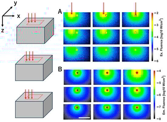
Figure 3. Fluence map of excitation (A) and fluorescence (B) for a fluorescent tumor embedded at a depth of 4 mm. The panels represent nine results obtained by varying the excitation light irradiation position. Three red arrows above the excitation maps indicate that the excitation light irradiation positions change along the X direction at 5 mm intervals from right to left. On the left side, three diagrams indicate that the excitation light irradiation positions change along the negative direction of the Y axis at 5 mm intervals from the center of the fluorescent tumor. (A,B) show the XZ cross-sectional view through the center of the fluorescent tumor. The white scale bar in the figure represents 20 mm. Color bars indicate fluence values on a logarithmic scale (log₁₀ W/cm²).

Figure 4 shows the results of calculating the two-dimensional position of the fluorescent tumor. The fluorescent tumor was embedded at a depth of 4 mm, with its center coordinates at (x, y) = (250, 250). Excitation light was irradiated at 25 positions arranged on a 20 × 20 mm area of the scattering medium surface, with 5 mm intervals between the points. Then, the coordinates of the fluorescent tumor were estimated based on the fluorescence intensity at the surface of the scattering medium obtained when excitation light was irradiated at four points: (200, 200), (300, 200), (200, 300), and (300, 300). The fluorescence intensities obtained at the four excitation light positions were 1.59 × 10⁻⁶, 1.57 × 10⁻⁶, 2.17 × 10⁻⁶, and 2.02 × 10⁻⁶ W/cm², respectively. The centroid coordinates were calculated based on the ratios of these four intensities. As a result, the distance between the embedded fluorescent tumor coordinates (250, 250) and the calculated centroid coordinates (248.84, 242.99) was 0.71 mm.

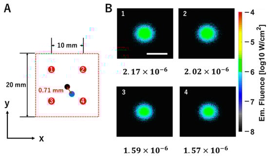
Figure 4. Evaluation of the accuracy of two-dimensional position estimation for the fluorescent tumor. (A) The left panel shows a top view of the 20 × 20 mm excitation light scanning area on the model surface (XY plane). The red circles labeled with the numbers 1–4 indicate the 4 excitation light irradiation coordinates used for the centroid calculation (1: (200, 300); 2: (300, 300); 3: (200, 200); 4: (300, 200)). The black circle represents the center coordinate of the embedded fluorescent tumor (250, 250), while the blue circle represents the centroid coordinate (248.84, 242.99) corresponding to the estimated position of the fluorescent tumor. The distance between these coordinates (indicated by the red arrow) is 0.71 mm. (B) Right panels are the fluorescence fluence maps on the model surface obtained by irradiating excitation light at each coordinate marked with red circles labeled 1–4. The white scale bar shown in the fluence map represents 20 mm. The fluorescence fluence values are shown at the bottom of each map (1: 2.17 × 10⁻⁶; 2: 2.02 × 10⁻⁶; 3: 1.59 × 10⁻⁶; 4: 1.57 × 10⁻⁶). The color bar indicates fluence values on a logarithmic scale (log₁₀ W/cm²).

Figure 5 shows the change in fluorescence fluence as the excitation light is scanned horizontally in 1 mm increments. As the light moved stepwise to the right relative to the center of the fluorescent tumor (top of Figure 5), the detected fluorescence fluence gradually decreased. Furthermore, the decrease in peak intensity was also observed through the regression line ($y=-0.25x+2.07,R^2=0.88$; bottom of Figure 5).

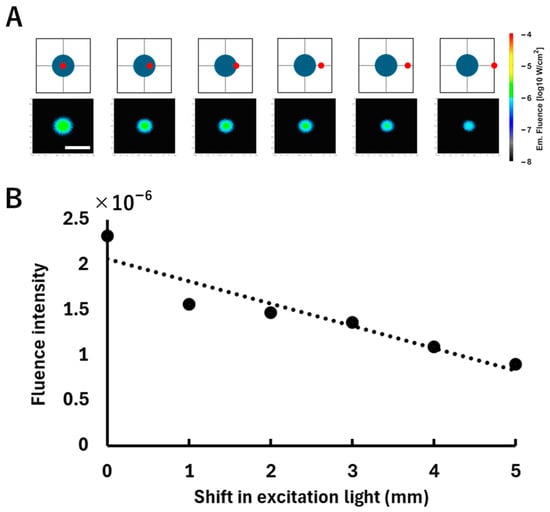
Figure 5. Relationship between the excitation light irradiation position shift and the fluorescence fluence. (A) The top row shows schematic illustrations of the excitation positions and the corresponding fluorescence fluence map on the surface of the model, displayed on a logarithmic scale (log₁₀ W/cm²). A spherical fluorescent tumor (blue) was positioned at a depth of 3 mm, where the excitation light (red) was incrementally shifted to the right from the tumor center at 1 mm intervals. The white scale bar shown in the fluence map represents 20 mm. (B) The bottom graph plots the average fluorescence fluence obtained from each fluence map. The horizontal axis indicates the lateral displacement of the excitation light from the tumor center, and the vertical axis indicates the corresponding average fluorescence fluence (W/cm²) calculated over a 10 × 10-pixel area centered at the centroid pixel of the fluorescence distribution. The dotted line is a regression line added to indicate the trend in the change in intensity.

3.1.2. Depth Estimation (Simulation Results)

Figure 6A presents the fluorescence simulation results when the fluorescent tumor was embedded at depths ranging from 1 to 6 mm. As the tumor depth increased, the fluorescence distribution became more diffuse due to scattering within the medium. Figure 6B shows the diffuse fluorescence profiles converted from the fluorescence fluence maps at each depth. It can be observed that the deeper the fluorescent tumor is embedded, the more the fluorescence spreads. Figure 7 presents the results of fitting using the analytical equation (Equation (2)), along with the estimated depths obtained (Figure 7A) and the error rates relative to the embedded tumor depths (Figure 7B). In Figure 7A, the horizontal axis represents the embedded depth ranging from 1 to 6 mm, while the vertical axis indicates the estimated depth. A strong correlation was observed between the embedded and estimated depths (R² = 0.98), indicating the validity of the fitting approach. In Figure 7B, the horizontal and vertical axes, respectively, represent the embedded depth and the error rate of the estimated depth relative to the embedded depth. In the tumor depth range of 1–6 mm, the error rate tends to decrease as the fluorescent tumor is embedded deeper. Additionally, in models with tumor depths beyond 7 mm, fluorescent tumor position estimation was performed by scanning the excitation light. However, when the tumor depth exceeded 7 mm, fluorescence could not be detected on the surface of the scattering medium. This is attributed to the low-excitation light intensity (0.5 mW) used for two-dimensional position estimation.

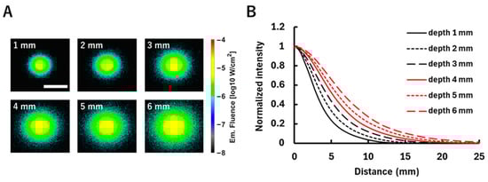
Figure 6. The fluorescence distribution for the fluorescent tumor embedded at different depths (1–6 mm). (A) Fluorescence fluence maps on the model surface when excitation light is irradiated directly above the fluorescent tumor at each depth. Fluence values are shown on a logarithmic scale (log₁₀ W/cm²). The white scale bar in the figure represents 20 mm. (B) Diffuse fluorescence profiles derived from the corresponding fluence maps. This shows the relationship between the distance from the excitation light irradiation position and the change in fluorescence fluence corresponding to that distance. The vertical axis is normalized to the maximum fluence at each depth.

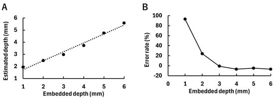
Figure 7. Results of depth estimation of the fluorescent tumor by fitting. (A) The relationship between the embedded depth of the fluorescent tumor and the estimated depth. The dotted line indicates a regression line ($y=0.74x+0.99$, $R^2=0.98$). (B) The relationship between the embedded depth of the fluorescent tumor and the error rate of the estimated depth relative to the embedded depth.

3.2. Limited Proof-of-Concept Experiment (Experimental Results)

3.2.1. Two-Dimensional Position Estimation (Experimental Results)

Table 2 presents the two-dimensional position estimation error of the fluorophore. With greater depths of the embedded fluorophore, sufficient fluorescence was detected for estimation even when the excitation light scanning interval was large. This is attributed to the fact that scattering in the intralipid solution increases with greater fluorophore depth. As a result, more excitation light reaches the fluorophore, inducing fluorescence emission. The estimation accuracy tends to decrease as the excitation light scanning interval increases.

Table 2. Two-dimensional position estimation accuracy of the fluorophore. The upper line shows the mean value, and the lower line shows the estimation errors for the three trials. The unit for both is millimeters (mm). The crosses in the table indicate that fluorescence was not detected.

	1 mm Interval	2 mm Interval	3 mm Interval	4 mm Interval	5 mm Interval
Depth 1 mm	0.34 (0.59, 0.29, 0.13)	1.39 (2.44, 0.89, 0.83)	×	×	×
Depth 2 mm	0.22 (0.28, 0.19, 0.20)	0.87 (0.58, 1.05, 0.98)	×	×	×
Depth 3 mm	0.15 (0.15, 0.14, 0.16)	0.46 (0.48, 0.44, 0.46)	1.75 (3.18, 0.78, 1.29)	×	×
Depth 4 mm	0.11 (0.22, 0.09, 0.02)	0.28 (0.66, 0.14, 0.04)	0.68 (1.35, 0.24, 0.45)	1.24 (1.11, 1.78, 0.84)	2.03 (3.38, 1.59, 1.13)
Depth 5 mm	0.16 (0.30, 0.01, 0.18)	0.38 (0.76, 0.12, 0.27)	0.76 (1.02, 0.55, 0.72)	1.52 (2.00, 091, 1.66)	1.38 (1.78, 1.44, 0.92)

3.2.2. Depth Estimation (Experimental Results)

Figure 8 shows the acquired images and the diffuse fluorescence profiles for each fluorophore depth. As shown in Figure 8A, the fluorescence spread with increasing fluorophore depth due to the effect of scattering. The diffuse fluorescence profiles in Figure 8B reflect the differences in fluorescence spread at each depth. Figure 9 shows the estimated fluorophore depths obtained by fitting, along with their error rates, with Figure 9A showing the estimated depth values corresponding to the depths at which the fluorophores were embedded. The plots indicate the averages of three experiments. The results of three experiments at each depth from 1 to 5 mm are as follows: a 1 mm depth: 1.19 mm, 1.85 mm, and 1.04 mm; a 2 mm depth: 2.20 mm, 1.83 mm, and 1.83 mm; a 3 mm depth: 2.75 mm, 2.71 mm, and 2.06 mm; a 4 mm depth: 3.34 mm, 3.62 mm, and 3.68 mm; and a 5 mm depth: 3.91 mm, 4.22 mm, and 4.27 mm. A strong correlation (R² = 0.99) was observed between the embedded fluorophore depth and the estimated depth. Figure 9B shows the error rates of the estimated depths relative to the embedded depths. The plots indicate the average error rates of the three experiments, which were within ±30%.

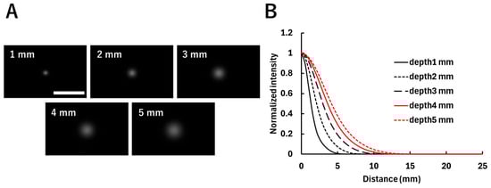
Figure 8. Fluorescence distribution of fluorophores embedded at different depths (1–5 mm). (A) Images acquired at each depth when the excitation light was irradiated directly above the fluorophore. The white scale bar in the figure indicates 20 mm. (B) Diffuse fluorescence profiles corresponding to each image, showing the relationship between the distance from the excitation light irradiation position and the corresponding fluorescence intensity. The vertical axis is normalized by the maximum fluorescence intensity at each depth.

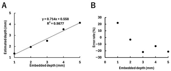
Figure 9. Results of the estimated depths of the fluorophore, with plots indicating the averages of three experiments. (A) Relationship between the embedded depth of the fluorophore and the estimated depth. The dotted line indicates the regression line (y = 0.71x + 0.56, R² = 0.99). (B) Relationship between the embedded depth of the fluorophore and the error rate of the estimated depth.

4. Discussion

4.1. Two-Dimensional Position Estimation (Simulation)

As shown in Figure 4, the distance between the embedded and estimated tumor coordinates at a depth of 4 mm was 0.71 mm. Zhou et al. examined the position estimation accuracy of a fluorescent source using FMT [24]. Here, the distance between the centroid of the embedded fluorescent target and that of the reconstructed image was approximately 0.2–0.3 mm. The results reported by Zhou et al. were superior to the estimation accuracy in the present study. However, FMT requires a large-scale setup and has a long computation time, thus limiting clinical implementation and real-time applicability. In contrast, our approach provides a faster and simpler estimation of the tumor position, which is advantageous for real-time clinical applications.

4.2. Depth Estimation (Simulation)

The depth estimation results obtained in the present study were compared with those reported in a previous study [7], in which the error rates for the estimated depths of fluorescent tumors ranging from 1 to 5 mm were generally within 25%. In contrast, as shown in Figure 7B, we found that the error rates for estimated depths from 1 to 5 mm were 93%, 24%, 1%, 7%, and 5%, respectively, confirming the tendency that shallower tumors, such as those at depths of 1–2 mm, are associated with larger estimation errors. This tendency can be attributed to insufficient fluorescence scattering in the shallow region, leading to a steeper diffuse fluorescence profile observed on the model surface (see Figure 6B). Therefore, the fitting accuracy with the analytical equation may have been reduced. In a previous study, an error of up to approximately 2 mm between the embedded and estimated depths was considered acceptable. In the present study, the maximum error obtained was 0.9 mm at a depth of 1 mm, which is sufficiently smaller than the error reported in the previous study. Alexa Fluor 647, which has an emission peak in the visible wavelength range (around 650 nm), was assumed in the previous study. Therefore, Alexa Fluor 647 does not penetrate deep into the medium compared to light in the near-infrared wavelength range. As a result, it may be difficult to estimate fluorescent tumors embedded deeper than 5 mm. In contrast, ICG, which has an emission peak in the NIR (around 820 nm), was assumed as the fluorescent dye in the present study. This enables the accurate depth estimation of tumors embedded deeper in the medium. In particular, as shown in Figure 7B, high estimation accuracy within a 10% error rate was achieved for depths between 3 and 5 mm. In a previous study [8], a depth-sensing imaging technique based on fluorescence time-of-flight was employed, enabling depth estimation with sub-millimeter resolution up to 5 mm. In the present study as well, the maximum depth estimation error was 0.9 mm at a depth of 1 mm, demonstrating accuracy comparable to that reported in the previous study. Furthermore, in the previous study, IRDye 680, which has an emission peak in the visible region, was used as the fluorescent dye. Therefore, depth estimation beyond 6 mm is difficult. In contrast, in the present study, ICG with an emission peak in the NIR region was assumed, allowing depth estimation up to 6 mm, which is slightly deeper. In another previous study [9], a deep-tissue imaging technique using excitation light scanning was developed. By extending the wavelength range into the SWIR region (1000–1700 nm), the estimation of fluorescent tumors embedded up to 50 mm deep in tissue was reported. In the present study, the positions of fluorescent tumors were estimated up to a depth of 6 mm using NIR wavelengths. Therefore, the previous study achieves a greater estimation depth. However, the SWIR wavelength range cannot be applied to clinical fluorescence tumor estimation because no fluorescent dyes in this wavelength range have been approved for clinical use.

4.3. Limits of Simulation

According to previous studies, in this simulation, it is assumed that the concentration distribution of the fluorescent dye within the tumor and the optical properties of the scattering medium are uniform [19,20]. By simplifying the model, the fundamental effectiveness of the fluorescent tumor position method was evaluated. However, in actual biological tissues, there are spatial variations in the concentration of fluorescent dye within the tumor and in the optical properties of normal tissues. Considering these factors, the fluorescence distribution and diffuse fluorescence profiles are expected to change, making depth estimation more complex. In the future, it will be necessary to construct a model considering these factors and evaluate their impact on the depth estimation of fluorescent tumors.

In the reflection configuration, fluorescence is assumed to be detected through the same optical path as the excitation light. However, since the simulation tracks only fluorescent photons, interference from the excitation light that occurs in experimental measurements is not considered. As a result, the obtained fluorescence fluence map is idealized.

In experiments, a dichroic mirror and a long-pass filter will be used in combination. The dichroic mirror separates 90% of the excitation light and fluorescence by wavelength. Furthermore, in front of the detector, a long-pass filter blocks 90% of the excitation light. Therefore, the interference from excitation light during fluorescence detection is considered to be minimized.

4.4. Effects of Optical Properties and Tumor Size

Depending on the optical properties of the model, the estimated depth may vary. According to [25], the absorption coefficient and scattering coefficient of brain tissue at 800 nm are reported to be 0.2 cm⁻¹ and 80 cm⁻¹, respectively. As shown in Table 1, the absorption and scattering coefficients of the intralipid solution at 800 nm are approximately 0.02 cm⁻¹ and 30 cm⁻¹. Thus, both coefficients are somewhat higher in brain tissue. If the optical properties of brain tissue were applied, the stronger absorption would decrease the fluorescence intensity, while the stronger scattering would broaden the full width at half maximum of the diffuse fluorescence profile. Consequently, the estimated depth may become a little larger. However, a comprehensive sensitivity analysis examining the effects of changes in the four optical properties, including the refractive index and anisotropy parameter, has not been conducted. Therefore, evaluating the robustness of the proposed method against optical properties that vary under physiological conditions remains a subject for future investigation.

To examine how tumor size affects depth estimation, simulations were performed only at a depth of 5 mm, varying the tumor diameter to 2, 4, and 6 mm. The estimated depths for each tumor size were 4.86, 4.75, and 4.99 mm, respectively. The range of these estimates was 0.24 mm. For the newly added fluorescent tumor sizes of 2 mm and 6 mm, the depth estimates showed smaller errors from the true depth of 5 mm than those for the 4 mm tumor. The effect of tumor size on the estimated depth was evaluated only at a depth of 5 mm, and was not investigated at other depths. Therefore, caution is required when generalizing the estimation accuracy at a depth of 5 mm to other depth–size combinations.

4.5. Comparison Between Simulation and Limited Proof-of-Concept Experiment

4.5.1. Two-Dimensional Position Estimation (Comparison)

In the simulation, the estimation error of the two-dimensional position at a depth of 4 mm was 0.71 mm when the excitation light was scanned at 5 mm intervals. As shown in Table 2, when the experimental scanning interval is set to the same 5 mm as in the simulation, the estimation error is 2.03 mm. Therefore, under the same scanning interval, the simulation showed higher estimation accuracy. However, in the experiments, reducing the excitation light scanning interval to 2 mm or less decreased the estimation error. These results indicate that while the simulation provides higher estimation accuracy when the excitation light scanning interval is the same at 5 mm, the experiments surpass the simulation in estimation accuracy as the scanning interval is reduced.

4.5.2. Depth Estimation (Comparison)

Figure 10 shows the fluorescence images obtained from the simulation and the experiments at depths of 1–5 mm. Both are fluorescence images used for depth estimation of the fluorophore, and the simulation images, converted to a linear scale, correspond to the fluence images in Figure 6A. The simulation images show more spread-out fluorescence than the experimental images, which is attributed to the difference in the effective attenuation coefficient (${\mu }_{\mathrm{e}\mathrm{f}\mathrm{f}}$) of the medium. In the simulation, the estimated ${\mu }_{\mathrm{e}\mathrm{f}\mathrm{f}}$ obtained from fitting was 0.30 ${\mathrm{m}\mathrm{m}}^{-1}$. This value represents the average of the estimated ${\mu }_{\mathrm{e}\mathrm{f}\mathrm{f}}$ across all depths. Similarly, the estimated ${\mu }_{\mathrm{e}\mathrm{f}\mathrm{f}}$ in the experiment was 0.64 ${\mathrm{m}\mathrm{m}}^{-1}$. Therefore, in tissues with an attenuation coefficient ranging from 0.30 to 0.64 mm⁻¹, the depth estimates are likely to be evaluated accurately. In a previous study [25], the attenuation coefficients of various brain regions at 800 nm were calculated using Equation (3). The wavelength of 800 nm is a representative value between the excitation wavelength of ICG at 785 nm and its fluorescence wavelength at 820 nm. As a result, the attenuation coefficients were 0.22 mm⁻¹ in the gray matter, 1.28 mm⁻¹ in the white matter, 0.68 mm⁻¹ in the cerebellum, 0.39 mm⁻¹ in the pons, and 0.53 mm⁻¹ in the thalamus. Therefore, in brain tissues other than the white matter and cerebellum, the depth can likely be estimated accurately. Therefore, under the constraints of tissue attenuation coefficients, the simulation demonstrates a reasonable approximation of the depth estimates observed in experiments.

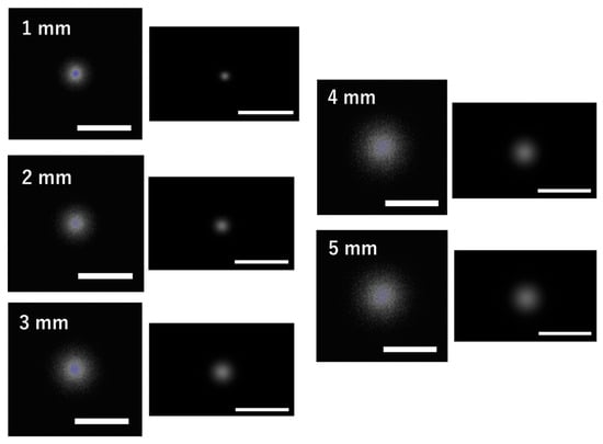
Figure 10. Comparison of fluorescence images between the simulation and the experiment. Fluorescence images from the simulation (left) and experiments (right) at fluorophore depths of 1–5 mm are shown. Each white scale bar indicates 20 mm.

4.5.3. Limits of Proof-of-Concept Experiment

This was performed using a simplified phantom and did not account for tissue het erogeneity, motion, or biological variability. Considering these points, the present experiment is regarded as a preliminary validation to demonstrate the effectiveness of the proposed method. Future investigations are required to evaluate the applicability of the method to biological tissue in actual clinical settings.

The maximum depth that can be estimated in the present study (simulation: 6 mm; experiment: 5 mm) remains limited compared with estimation methods targeting deeper tissues [9].

4.6. Beer’s Law Under Scattering Conditions

Beer’s law, which was used in this study, describes the attenuation of light due to absorption in a medium. Dang et al. reported a study that utilized Beer’s law, in which light propagating through a scattering medium attenuates exponentially with optical pathlength [9]. The original form of Beer’s law may not be suitable in models where scattering is dominant. Previous time-resolved spectrophotometry studies have demonstrated that, even when photons travel along nonlinear paths due to strong scattering, their intensity decays exponentially as a result of absorption [26]. This study indicates that, when considering the microscopic paths of photons, absorption-induced attenuation is independent of the degree of scattering and can be described as an exponential decay regardless of scattering effects. Furthermore, when this relationship is extended to continuous illumination, the apparent optical pathlength through tissue is not affected by physiological variations in absorption. In this study, because the absorption coefficient is defined as a constant, the light intensity in the scattering medium can be approximated using exponential attenuation. Therefore, this analytical equation does not fully capture the complexity of photon transport in biological tissue with heterogeneous optical properties.

4.7. Application to the SWIR Wavelength Range

By updating the simulation parameters to those appropriate for SWIR wavelengths, our method can be applied to the SWIR wavelength range. It has been documented that extending the wavelength range to SWIR allows light to penetrate deeper into the medium compared to NIR wavelengths [27]. In the present method, the excitation light intensity was set to 0.5 mW, which corresponds to the maximum intensity that does not saturate the fluorescence intensity at a depth of 1 mm in the experimental measurements. Consequently, the estimation of the two-dimensional position and depth could only be achieved down to 6 mm. However, by using SWIR fluorescent dyes and corresponding SWIR light sources, it may be possible to obtain sufficient fluorescence for detection even beyond 7 mm, enabling two-dimensional position and depth estimation. However, the SWIR wavelength range cannot be applied to clinical fluorescence tumor estimation because no fluorescent dyes in this wavelength range have been approved for clinical use.

5. Conclusions

In this study, we proposed a method for three-dimensional position estimation of a fluorescent tumor using an excitation light scanning configuration and evaluated its feasibility using Monte Carlo simulations. A voxel model simulating the scattering characteristics of biological tissue was created. In a two-dimensional position estimation of the fluorescent tumor, we investigated how the distance between the tumor and the excitation light positions affects the excitation and fluorescence fluence. Then, the distance between the coordinates of the embedded fluorescent tumor and the estimated coordinates was calculated to evaluate the accuracy of the two-dimensional position estimation. The fluorescent tumor depth was estimated by fitting an analytical equation to the fluorescence distribution obtained on the model’s surface. In the simulation, the estimated tumor depths of 2–6 mm showed high-precision agreement with the embedded depths, with an error rate of approximately 20%. In previous studies [7], depth estimation was limited to 1–5 mm using visible light, but in the present study, the use of longer wavelengths enabled estimation at slightly greater depths. This limited proof-of-concept study was conducted using an experimental system. The simulations, when compared with the experimental measurements, did not produce any inconsistencies. In the estimation of the two-dimensional position of the fluorophore, it was observed that the estimation error tended to decrease as the excitation light scanning interval became smaller. The simulation provides higher estimation accuracy when the excitation light scanning interval is 5 mm. However, the experiments surpass the simulation in estimation accuracy as the scanning interval is reduced. In depth estimation, the estimation error relative to the embedded depth remained within ±30%. By comparing the results of simulations and the experiment, the range of tissue attenuation coefficients for which depth estimation can be accurately evaluated was determined. Overall, the proposed method would be most suitable for applications involving shallow tumors or intraoperative lesions accessible from the body surface.

References

- Uddin, M.J. Advances in imaging retinal inflammation. Exp. Eye Res. 2025, 259, 110537. [Google Scholar] [CrossRef] [PubMed]
- Mehravanfar, H.; Farhadian, N.; Abnous, K.; Zavvar, T. Catalase enzyme-modified carbon quantum dot nanoparticles with hypoxia alleviation associated with indocyanine green for synchronous augmented photodynamic therapy and cell imaging of melanoma. Nanoscale 2025, 17, 19631–19655. [Google Scholar] [CrossRef] [PubMed]
- Schouw, H.M.; Huisman, L.A.; Janssen, Y.F.; Slart, R.H.J.A.; Borra, R.J.H.; Willemsen, A.T.M.; Brouwers, A.H.; van Dijl, J.M.; Dierckx, R.A.; van Dam, G.M.; et al. Targeted optical fluorescence imaging: A meta-narrative review and future perspectives. Med. Mol. Imaging 2021, 48, 4272–4292. [Google Scholar] [CrossRef] [PubMed]
- Wang, G.; Li, W.; Shi, G.; Tain, Y.; Kong, L.; Ding, N.; Lei, J.; Jin, Z.; Tain, J.; Du, Y. Sensitive and specific detection of breast cancer lymph node metastasis through dual-modality magnetic particle imaging and fluorescence molecular imaging: A preclinical evaluation. Med. Mol. Imaging 2022, 49, 2723–2734. [Google Scholar] [CrossRef]
- Miller, J.P.; Maji, D.; Lam, J.; Tromberg, B.J.; Achilefu, S. Noninvasive depth estimation using tissue optical properties and a dual-wavelength fluorescent molecular probe in vivo. Biomed. Opt. Express 2017, 8, 3095–3109. [Google Scholar] [CrossRef]
- Stuker, F.; Ripoll, J.; Rudin, M. Fluorescence molecular tomography: Principles and potential for pharmaceutical research. Pharmaceutics 2011, 3, 229–274. [Google Scholar] [CrossRef]
- Kolste, K.K.; Kanick, S.C.; Valdes, P.A.; Jermyn, M.; Wilson, B.C.; Roberts, D.W.; Paulsen, K.D.; Leblond, F. Macroscopic optical imaging technique for wide-field estimation of fluorescence depth in optically turbid media for application in brain tumor surgical guidance. J. Biomed. Opt. 2015, 20, 26002. [Google Scholar] [CrossRef]
- Petusseau, A.F.; Streeter, S.S.; Ulku, A.; Feng, Y.; Samkoe, K.S.; Bruschini, C.; Charbon, E.; Pogue, B.W.; Bruza, P. Subsurface fluorescence time-of-flight imaging using a large-format single-photon avalanche diode sensor for tumor depth assessment. J. Biomed. Opt. 2024, 29, 016004. [Google Scholar] [CrossRef]
- Dang, X.; Bardhan, N.M.; Qi, J.; Gu, L.; Eze, N.A.; Lin, C.W.; Kataria, S.; Hammond, P.T.; Belcher, A.M. Deep-tissue optical imaging of near cellular-sized features. Sci. Rep. 2019, 9, 3873. [Google Scholar] [CrossRef]
- Iida, T.; Kiya, S.; Kubota, K.; Jin, T.; Seiyama, A.; Nomura, Y. Monte Carlo modeling of shortwave-infrared fluorescence photon migration in voxelized media for the detection of breast cancer. Diagnostics 2020, 10, 961. [Google Scholar] [CrossRef]
- Yuan, B.; Chen, N.; Zhu, Q. Emission and absorption properties of indocyanine green in Intralipid solution. J. Biomed. Opt. 2004, 9, 497–503. [Google Scholar] [CrossRef] [PubMed]
- Moran, L.J.; Wordingham, F.; Gardner, B.; Stone, N.; Harries, T.J. An experimental and numerical modelling investigation of the optical properties of Intralipid using deep Raman spectroscopy. Analyst 2021, 146, 7601–7610. [Google Scholar] [CrossRef] [PubMed]
- Grabtchak, S.; Palmer, T.; Foschum, F.; Liemert, A.; Kienle, A.; Whelan, W.M. Exprimental spectro-angular mapping of light distribution in turbid media. J. Biomed. Opt. 2012, 17, 067007. [Google Scholar] [CrossRef] [PubMed]
- Lai, P.; Xu, X.; Wang, L.V.; Liemert, A.; Kienle, A.; Whelan, W.M. Dependence of optical scattering from Intralipid in gelatin-gel based tissue-mimicking phantoms on mixing temperature and time. J. Biomed. Opt. 2014, 19, 035002. [Google Scholar] [CrossRef]
- Iida, T.; Jin, T.; Nomura, Y. Monte Carlo Modeling of Near-infrared Fluorescence Photon Migration in Breast Tissue for Tumor Prediction. Adv. Biomed. Eng. 2020, 9, 100–105. [Google Scholar] [CrossRef]
- Lu, L.; Li, B.; Ding, S.; Fan, Y.; Wang, S.; Sun, C.; Zhao, M.; Zhao, C.; Zhang, F. NIR-II bioluminescence for in vivo high contrast imaging and in situ ATP-mediated metastases tracing. Nat. Commun. 2020, 11, 4192. [Google Scholar] [CrossRef]
- Weng, D.; Jin, X.; Qin, S.; Lan, X.; Chan, C.; Sun, X.; She, X.; Dong, C.; An, R. Radioimmunotherapy for CD133(+) colonic cancer stem cells inhibits tumor development in nude mice. Oncotarget 2017, 8, 44004–44014. [Google Scholar] [CrossRef]
- Sitia, L.; Sevieri, M.; Bonizzi, A.; Allevi, R.; Morasso, C.; Foschi, D.; Corsi, F.; Mazzucchelli, S. Development of Tumor-Targeted Indocyanine Green-Loaded Ferritin Nanoparticles for Intraoperative Detection of Cancers. ACS Omega 2020, 5, 12035–12045. [Google Scholar] [CrossRef]
- Ong, Y.H.; Finlay, J.C.; Zhu, T.C. Monte Carlo modelling of fluorescence in semi-infinite turbid media. Proc. SPIE Int. Soc. Opt. Eng. 2018, 10492, 104920T. [Google Scholar] [CrossRef]
- Kervella, M.; Humeau, A.; Huillier, J.P. Time-resolved fluorescence intensity issued from a heterogeneous slab: Sensitivity characterization. Opt. Commun. 2008, 281, 5982–5990. [Google Scholar] [CrossRef]
- Wang, L.; Jacques, S.L.; Zheng, L. MCML—Monte Carlo modeling of light transport in multi-layered tissues. Comput. Methods Programs Biomed. 1995, 47, 131–146. [Google Scholar] [CrossRef]
- Matsumoto, M.; Nishimura, T. Mersenne Twister: A 623-dimensionally equidistributed uniform pseudorandom number generator. ACM Trans. Model. Comput. Simul. 1998, 8, 3–30. [Google Scholar] [CrossRef]
- Jacques, S.L. Handbook of Biomedical Fluorescence, 1st ed.; CRC Press: Boca Raton, FL, USA, 2003; p. 45. [Google Scholar] [CrossRef]
- Zhou, T.; Ando, T.; Nakagawa, K.; Liao, H.; Kobayashi, E.; Sakuma, I. Localizing fluorophore (centroid) inside a scattering medium by depth perturbation. J. Biomed. Opt. 2015, 20, 017003. [Google Scholar] [CrossRef]
- Schwarzmaier, H.; Yaroslavsky, A.N.; Yaroslavsky, I.V.; Goldbach, T.; Kahn, T.; Ulrich, F.; Schulze, P.C.; Schober, R. Optical properties of selected native and coagulated human brain tissues in vitro in the visible and near infrared spectral range. Phys. Med. Biol. 2002, 47, 2059. [Google Scholar] [CrossRef]
- Nomura, Y.; Hazeki, O.; Tamura, M. Relationship between time resolved and non-time-resolved Beer-Lambert law in turbid media. Phys. Med. Biol. 1997, 42, 1009–1022. [Google Scholar] [CrossRef]
- Cosco, E.D.; Arus, B.A.; Spearman, A.L.; Atallah, T.L.; Lim, L.; Leland, O.S.; Caram, J.R.; Bischof, T.S.; Bruns, O.T.; Sletten, E.M. Bright Chromenylium Polymethine Dyes Enable Fast, Four-Color In Vivo Imaging with Shortwave Infrared Detection. J. Am. Chem. Soc. 2021, 143, 6836–6846. [Google Scholar] [CrossRef]
Disclaimer/Publisher’s Note: The statements, opinions and data contained in all publications are solely those of the individual author(s) and contributor(s) and not of MDPI and/or the editor(s). MDPI and/or the editor(s) disclaim responsibility for any injury to people or property resulting from any ideas, methods, instructions or products referred to in the content. |
© 2025 by the authors. Licensee MDPI, Basel, Switzerland. This article is an open access article distributed under the terms and conditions of the Creative Commons Attribution (CC BY) license.