Abstract
Existing reinforced concrete (RC) buildings in Europe have generally been designed without proper consideration of seismic actions and capacity design principles, and thus they tend to be vulnerable to earthquakes. Moreover, since a significant proportion of the aforementioned buildings were developed during the 1950s and 1960s, they are currently close to the end of their service life. Therefore, seismic assessment of existing RC building is a major issue in structural engineering and construction management, and the related seismic analyses should take into account the effect of material ageing and degradation. This paper proposes a practice-oriented procedure for quantifying seismic reliability, taking into account the main effects of carbonation-induced degradation phenomena. It summarizes the main aspects of the most up-to-date models for the seismic degradation of concrete and RC members and shows how nonlinear static (pushover) analyses can be utilized (in lieu of the most time-consuming non-linear time history analyses) in quantifying seismic reliability with respect to the performance levels of relevance in seismic engineering. A relevant case study is finally considered with the aim to showing how some parameters, such as exposure class and cover thickness, affect the resulting seismic reliability of existing RC buildings.
1. Introduction
In Europe, the vast majority of reinforced concrete (RC) structures were built in areas classified as non-seismic at the time of construction and before seismic codes came into force [1]. Moreover, they are generally close to the end of their design service life, as their construction periods generally date back to the post-WWII period [2].
Furthermore, a huge number of these structures may be affected by severe material degradation phenomena, since classical procedures adopted in concrete structure design have often failed to achieve sufficiently durability [3]. Consequently, both designing durable RC structures and handling the degradation phenomena possibly developing in existing ones are timely challenges in modern structural engineering [4].
In the last few decades, great effort has been spent in the mathematical modelling of corrosion induction due to different degradation phenomena, such as carbonation, chloride ingress, alkali aggregate reaction and frost [5]. A series of parametric studies have been performed in order to formulate semi-probabilistic and full-probabilistic methods, which are applicable for service life design purposes and for existing objects, including the effects of both environmental and material parameters (that may require proper structural investigation) [6].
A relevant consequence of such studies was the introduction of environmental exposure conditions for concrete structures in EN 1992-1-1:2004 [7], with the aim being to introduce practice-oriented criteria regarding the choice of both material properties and the proper concrete cover thickness.
Among the various degradation phenomena of relevance, carbonation-induced degradation is certainly the most common, as all RC structures are exposed to atmospheric CO2. Although it may induce milder degradation effects than other phenomena (e.g., chloride ingress) possibly affecting steel rebars [8], it is more widespread and leads to carbonation of the concrete cover, resulting in depassivation and, consequently, reinforcement corrosion.
Experimental tests carried out on RC members have shown that their load carrying capacity, together with their ductility properties, decrease as the level of rebar corrosion increases [9]. Several studies have been developed with the aim being to propose modified constitutive laws in order to take into account material degradation phenomena affecting both concrete and reinforcement [10].
Moreover, other formulations have been proposed in order to quantify the influence of rebar corrosion on member capacity [11]. Recent numerical simulations of structural seismic behaviour (in terms of Pushover curves), considering the effects of carbonation-induced degradation at different ages of the structural life, clearly demonstrated a pronounced capacity degradation, confirming that the observed cross sectional strength reduction reverberates its effects upwards at the structural scale [12].
In principle, the safety and serviceability assessment of RC structures should consider the time-dependent variation of the structural response due to degradation phenomena [13]. Adopting a fibre discretisation of transverse sections, it is easy to implement the progressive effects of material degradation (in terms of loss of concrete cover and the reduction in steel rebar area) in the structural model [14].
In reality, the increasing deterioration of concrete as well as the progressive corrosion of reinforcing bars may lead to significant a reduction in structural reliability, with respect to the initial values at both ultimate and serviceability limit states [13].
The “2000 SAC/FEMA” is one of the most well-established reliability and risk assessment methods, specialised for seismic problems [15,16]. This method aims to provide a closed-form (and easy to compute) expression for the risk, written according to the classical reliability formulations.
Although the original formulation of the SAC/FEMA method does not take into account the time-dependent variation of the structural response, possibly due to degradation phenomena, recent extensions have been proposed, with the aim being to include the time-variant nature of the structural response [17]. Specifically, this evolution leads to defining an “equivalent constant rate” (ECR) of degradation, which allows for maintaining a code-compatible format based on the mean annual frequencies (MAFs) of exceedance.
The aforementioned procedures provide structural engineers with somewhat simplified methodologies for the assessment of seismic risk, namely the mean annual probability PLS of a structure to achieve a given limit state (LS) as exposed to a seismic hazard described by hazard curves.
In addition to their simple conceptual framework, they require carrying out a huge number of non-linear time history analyses that are increasingly time-consuming as the level of detail of the numerical models increases, as is usually required to achieve a sufficient accuracy in simulating the structural response of the existing structures. In particular, incremental dynamic analyses (IDA) have to be carried out on structures with the aim to obtain a “median” relationship between a seismic “intensity measure” (IM) and a relevant “engineering demand parameter” (EDP) and the corresponding dispersion due to record-to-record variability [18].
However, in the scientific literature, simple alternatives to IDA have been proposed. Both procedures rely on the application of the N2 method [19], considering demand spectra characterized by an increasing value of the intensity parameter (namely, the pseudo-acceleration at the fundamental period of vibration of the structure) with the aim of directly obtaining the relationship between the seismic demand D and the intensity measure Sa. On the one hand, the so-called “incremental N2 method” (IN2) [20] considers design spectra to obtain the average relationship between IM and EDP, whereas an alternative proposal is based on representing demand by means of a set of natural spectra with the aim of reproducing the record-to-record variability [21].
Moreover, three different (ideally alternative) methods of seismic reliability assessment of RC and masonry structures are proposed in CNR-DT 212/2013 [22]. The main difference between those methods consists of the suggested analysis methodology, together with the required computational effort. Recent comparative analyses among these methods were developed with the aim of validating the simpler methodologies, based on static analyses, comparing their results with the outcomes of dynamic analyses, which are meant to be the most accurate ones [23].
The present paper proposes a general practice-oriented framework and some preliminary results about the evaluation of seismic reliability of RC structures affected by carbonation-induced degradation phenomena. To this end, a simple yet mechanically consistent implementation of the effects of material degradation in a structural analysis model is described. Then, the results obtained for nonlinear static (pushover) analyses are utilised to obtain reliability evaluations by means of well-established methodologies. The outcomes of some parametric analyses are presented in order to quantify the evolution of PLS (seismic risk) resulting from alternative scenarios involving different environmental exposures, material properties and structural detailing in terms of concrete cover.
2. Outline of Theoretical Models for Carbonation-Induced Degradation Phenomena
Since carbonation-induced degradation can have a great impact on the structural behaviour, recently, new conceptual frameworks have been formulated with the aim of designing the service life of new RC structures and analysing existing ones by taking into account the degradation processes possibly induced by environmental exposure [24]. The fib Model Code 2010 [25] provides researchers and practitioners with a wide report of the most recent models available in the literature for simulating the degradation processes and their consequences on the structural response of members and structures.
2.1. Carbonation and Corrosion Models
In this context, the well-known Tuutti’s model for the degradation of structures is a classical conceptual tool employed to describe the time-evolution of the effects of concrete degradation in RC sections [26].
The diffusion of carbonation inside concrete covers is generally derived from the well-known Fick’s law. The depth of the carbonated layer of concrete can be expressed as a function of the square root of time t, and the following expression can be obtained for the depassivation time td [24]:
where:
- -
- ke is environmental function (-);
- -
- kc is execution transfer parameter (-);
- -
- kt is regression parameter (-);
- -
- RACC,0−1 is inverse effective carbonation resistance of concrete ((mm2/years)/(kg/m3));
- -
- εt is error term;
- -
- Cs is the CO2 concentration (kg/m3);
- -
- Wt is the weather function, intended at simulating the effects of driving rains on carbonation of the member under consideration (-).
It is worth highlighting that RACC,0−1 is strongly related to the chemical composition of concrete, which can be represented by an “equivalent water cement ratio”, as defined in [27]. In particular, RACC,0−1 decreases as the water cement ratio decreases. Consequently, a proper consideration of water cement ratio at design stage can increase the structure durability itself.
Further relevant information about mathematical expressions and statistical definitions assumed for the above parameters can be found in the original work [6].
Depassivation ideally triggers oxidation and, hence, the corrosion of steel reinforcements. A linear model can be considered to describe the time evolution of bar radius loss xcorr as follows [25]:
where the two parameters Vcorr and wt, representing the rate of corrosion and a weather function, depend on the environmental exposure class which the member is subjected to [5].
As for concrete cracking and spalling, crack width is supposed to grow linearly right after td, and a conventional value wcr = 0.05 mm is assumed to define “visible” crack opening. Specifically, the following expression is assumed in the present study:
where:
- -
- β is a parameter controlling propagation (-);
- -
- p (t − td) is a measure of the propagation phenomenon (mm), which can be equalled to the loss of radius in steel bars xcorr(t).
The following expression is assumed for p0:
where:
- -
- (d’ − ϕ/2)/ϕ is the ratio between the initial concrete cover and the initial bar diameter (mm);
- -
- ft,sp is the splitting strength of concrete;
- -
- a1, a2, and a3 are calibration parameters.
Consequently, the value tcr can be obtained by solving Equation (2) with respect to time t and after imposing xcorr(tcr) = p0 given by Equation (4). The values assumed for both β in Equation (3) and a1, a2, and a3 in Equation (4) are consistent with the mean and regression values determined as part of the DuraCrete Project [28]. Then, the splitting condition in the concrete cover can be determined when w in Equation (3) reaches a given threshold limit, which in the present study is assumed as ws = 1 mm. The value of ts (spalling time) can be easily derived by solving Equation (3) with respect to t, for w = 1 mm.
Therefore, Equations (1)–(4) can completely describe the time evolution of the relevant degradation phenomena driven by concrete carbonation, which lead, on the one hand, to a reduction in bar radius (from td on) and, on the other hand, to the (linearly) progressive loss of concrete cover between times tcr and ts.
Finally, it is worth highlighting that the models summarised above are utilised in a deterministic way, with the aim being to understand the influence of the relevant parameters of the member and structural response in RC frames. However, the parameters controlling Equations (1)–(4) need to be defined in statistical terms with the aim of covering both uncertainty and randomness affecting their predictions.
2.2. Influence of Rebar Corrosion on the Chord Rotation
It is expected that material degradation can affect the member capacity under seismic actions. Recent studies highlighted that steel corrosion not only causes a reduction in the cross-sectional area of rebars, but also shows similar effects on the ductility and on stress–strain relationships of the corroded reinforcement [11]. Many formulations have been proposed in order to take into account the decrease in both capacity and ductility of reinforcement [10].
Moreover, extending these observations to the structural behaviour of ageing structures, it is worthwhile to account for a reduction in capacity in terms of chord rotation, which becomes higher as the mass loss (ψ) of reinforcement increases. This correction of the time-independent capacity formulations could be provided by a bilinear formulation:
The parameters of this bilinear formulation depend on the longitudinal rebar diameter and are available in [11]. In each case, the capacity decay is more pronounced for values of mass loss less than ψlim = 10%.
3. Outline of the Bases of Reliability Analysis
3.1. Risk Evaluation Methods
3.1.1. The “2000 SAC/FEMA” Method
This framework aims to provide criteria based on desired performance objectives, which are defined as specified probabilities of exceeding a certain performance level.
To do so, the probabilistic representations of the three aforementioned elements are needed. Normally the general design approach considers demand “D” and capacity “C” separately, comparing them in two steps at the displacement or drift level.
The method relies on the following hypotheses:
- the pseudo-acceleration value Sa(Tf) corresponding to a period T close to the fundamental period of the structure Tf is often assumed as the intensity measure (IM) for seismic signals which can be scaled for covering the entire relevant integration domain;
- to quantify seismic response of structures, a consistent engineering demand parameter (EDP) is defined. While a comparative analysis of those parameters can be found in [29], in the present paper, chord rotation is considered as the demand measure, as usually adopted in similar applications;
- demand “D” is a log-normal random variable, characterized by the median value . The relationship between the intensity measure sa and the median demand is assumed to be a power law, as follows:
This regression curve should be combined with the drift capacity representation and with the hazard function to produce PLS, the annual probability of achieving a certain limit state (e.g., collapse or life safety level). Probabilistic seismic hazard analysis (PSHA) defines (on regional basis) the hazard function H(sa), which gives the annual probability that the (random) intensity Sa at the site will be equal to or exceed the level sa. This curve can be reasonably approximated as follows:
Using the total probability theorem, it is possible to express the drift hazard curve HD(d): the MAF that the drift demand D exceeds any specified value d, given an intensity measure Sa from the hazard curve. In discrete form, the drift hazard curve is given by:
having expanded the probability of interest by conditioning on all possible levels of ground motion.
Based on the above hypotheses, the following expression can be derived for the probability of the structure to achieve the limit state LS, as shown in [21];
The probability obtained through Equation (9) is basically obtained as the product of two factors whose meaning can be easily understood:
- is the annual probability of occurrence of an earthquake whose intensity Sa is larger than the value sa, which corresponds to a median demand equal to median capacity for a given Limit State (. Hence, this term represents the probability for the structure to achieve the LS of interest considering both capacity and demand as deterministic variables: the former one is defined as a function of the geometric and mechanical model of the structure members and the latter one is basically defined as a function of the seismic intensity measure;
- represents a magnification factor (MF) accounting for the probabilistic nature of seismic demand (the “record-to-record” variability, related to the accelerograms chosen for the analyses) and structural capacity. In particular and represent the variances of demand and capacity (associated with a certain LS), both regarded as random variables log-normally distributed.
Moreover, assuming that capacity is deterministic, its eventual dispersion around the median value is neglected for each limit state. Thus, the abovementioned PLS turns in the following expression, where obviously the magnification factor takes into account only the probabilistic nature of seismic demand:
3.1.2. The Equivalent Constant Rate (ECR)
The concepts of exceedance probabilities of “10% in 50 years” integrated into our design methodologies may be modified as degradation phenomena occur.
This concept represents a homogeneous Poisson process with a constant rate of PLS, which gives the probability “p” of exceedance over the lifetime of Td years as
Nevertheless, the assumption of a constant rate PLS may not be adequate for all the structures that are subjected to relevant environmental actions, that slowly degrade their capacity over time. As time increases and the degradation phenomena takes place, not only does the median capacity of the structure decrease, but also the uncertainties associated with the degradation process may change.
Vamvatsikos and Dolšek [17] clearly showed that, when the rate of degradation is relatively close to linear, it is possible to derive simple formulations aiming to describe an equivalent constant rate (ECR) associated with the lifetime Td, approximately equal to the service life of the structure itself.
where:
- -
- PLS(t) expresses the time-evolution of PLS and, according to the authors, could be approximately derived from the regression parameters that describe the evolution of seismic demand and its dispersion during time;
- -
- α is the societal discount rate, which can be fixed for instance at 0.1%. In this case, the ECR will be approximately equal to the average rate, defined in the following lines.
Alternatively, it is possible to evaluate an average rate (AVG) applying the median theorem at PLS(t) on the whole range [0, Td].
Assuming that structure capacity degradation during the time period is described by a power law and that the dispersion increases linearly with time, it is possible to derive a closed-form expression of ECR. The complete analytical formulation is available in [17].
3.2. Analysis Procedure
3.2.1. Use of Nonlinear Static (Pushover) Analysis
In order to formulate a practice-oriented procedure, the first contribution introduced by the present paper consists of extending the use of pushover analysis to seismic reliability assessment, considering its cost-effectiveness in terms of computational costs with respect to the usual procedures based on dynamic analysis [21].
In particular, among the analysis methodologies proposed in CNR-DT 212/2013 [22], “Method C” is employed herein. Recent research showed that “Method C” can lead to an estimation close to that of “Method A”, which is thought to be more accurate [23].
However, it is necessary to evaluate the variability of seismic demand, employing natural spectra, directly derived by the same recorded accelerograms which could have been utilized for time-history analyses in IDA. Natural spectra, with their rough shape, can be directly utilized to apply the N2 method, with the aim of reproducing the record-to-record variability, which is typical of time-history analyses.
The method proposed in the present paper relies on the availability of a pushover curve representative of the inelastic behaviour of the structure. In order to simulate the inelastic response of the frame, it may be suitable to adopt a fibre formulation model that distributes plasticity by means of numerical integrations through the member cross sections and along the member length. In the present work, a concentrated-plasticity model is adopted for beam elements, making use of the OpenSEES [14] “beam with hinges” element, while the distributed-plasticity OpenSEES “nonlinear beam-column” element is employed to model column behaviour.
Uniaxial material models are defined to capture the nonlinear hysteretic axial stress–strain characteristics in the cross sections. The plane-sections-remain-plane assumption is enforced, where uniaxial material “fibres” are numerically integrated over the cross section to obtain stress resultants (axial force and moments) and incremental moment–curvature and axial force–strain relationships. The cross sectional parameters are then integrated numerically at discrete sections along the member length, using displacement or force interpolation functions [30,31].
3.2.2. Seismic Demand Determination
As anticipated in the previous paragraph, for each natural spectrum, the spectral ordinates (in terms of acceleration) should be divided according to the spectral acceleration Sa(Tf) corresponding to the natural period of vibration Tf. Consequently, it is possible to scale the natural spectra in order to cover the entire relevant integration domain.
The displacement demand for the SDOF (whose period of vibration is T*) equivalent to the given MDOF structure can be easily derived making use of the N2 method, providing reasonably accurate results [19]:
where
- -
- μ is the ductility factor, defined as the ratio between the maximum displacement and the yield displacement;
- -
- Rμ is the reduction factor due to ductility (i.e., due to hysteretic energy dissipation of ductile structures);
- -
- T0 is the transition period, which is assumed to be equal to the characteristic period TC, which represents the intersection between the constant pseudo-acceleration branch and the constant pseudo-velocity one according to the Newmark and Hall idealization of seismic spectra [32].
For each spectrum, the reference period TC is calculated as follows:
where max(SV) and max(Sa) are, respectively, the maximums of the spectral velocity and the spectral acceleration.
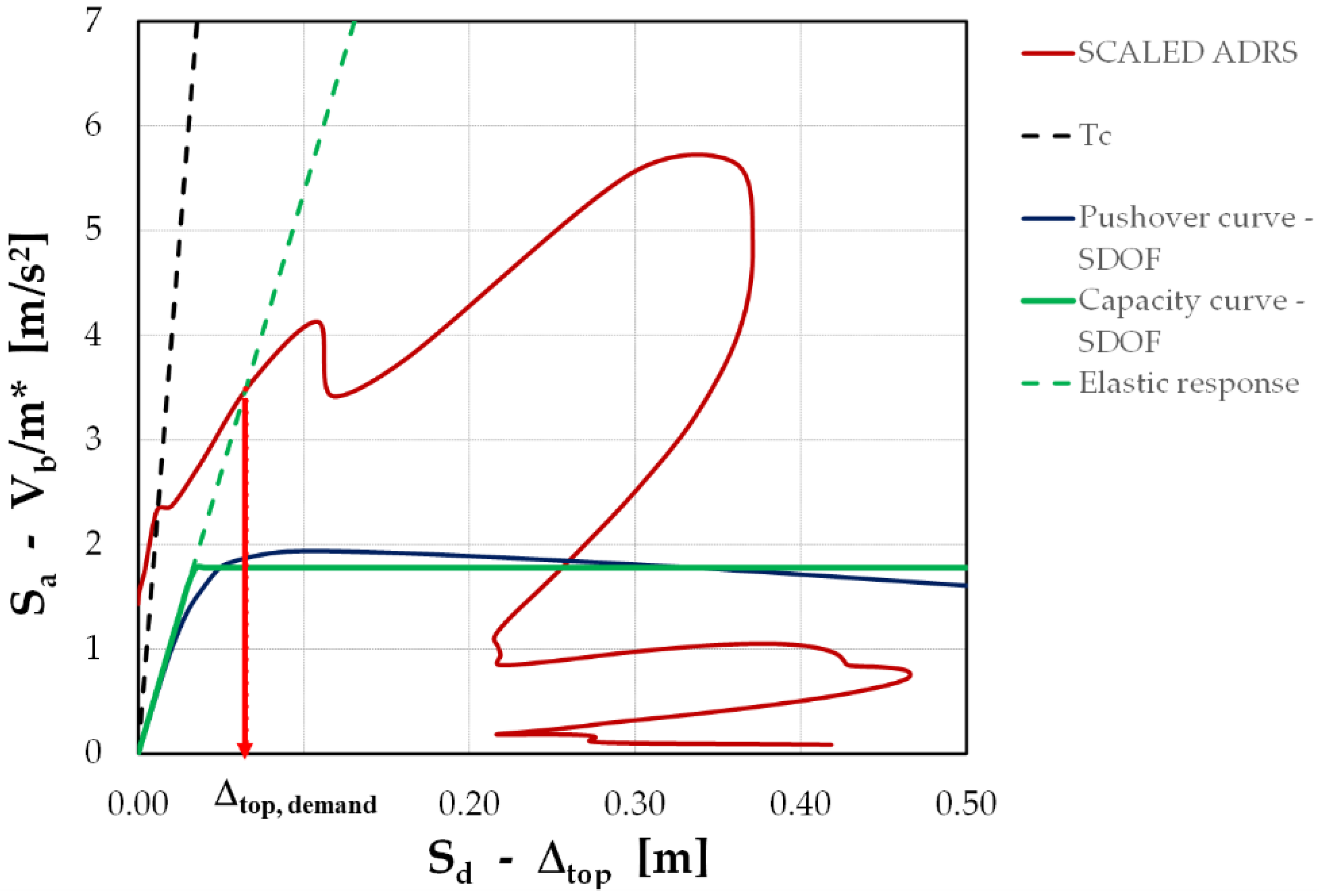
Figure 1 represents a sample (graphical) application of the N2 method employing one natural spectrum characterizing a characteristic period TC = 0.45 s, scaled by a scale factor (SF) equal to 2.75 m/s2. The elastic demand spectrum is represented in the ADRS format, while the capacity curve is represented in terms of Vb/m* (ratio between base shear force and participant mass) and Δtop (top displacement). Since T* is approximately equal to 0.85 s, the equal-displacement rule is applied—Equation (16)—in order to determine the seismic displacement demand Δtop, demand.
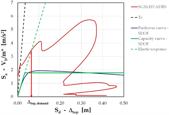
Figure 1.
Sample application of N2 method in the case of TC = 0.45 s.
3.2.3. Evaluation of the PLS and Extension to the Case of Ageing Structures
Firstly, the seismic demand is evaluated for each accelerogram and for different values of the scaling factor compatible with structure displacement capacity.
Then, it is necessary to evaluate not only the intensity measures (IM) corresponding to the EDP associated with each limit state using Equation (6), but also the dispersion (namely, the variance of the log-normal random variable “D”) at each relevant level of IM.
As previously anticipated, the second contribution introduced by the present paper regards the evaluation of dispersion measures, using static analyses rather than incremental dynamic ones. Dispersion is measured by means of variance β2D of the random variable “D” (demand), regarded as log-normally distributed.
Thus, it is possible to compute the PLS for each relevant limit state using Equation (10). To this end, the evaluation of the maximum of chord rotation (EDP, lim) for each limit state is realized following the prescription of CNR-DT 212/2013 [22].
As highlighted in Section 2.2, the maximum values of chord rotation (EDP, lim) also depend on the mass loss of rebars, since they are determined by means of Equation (5).
The third contribution presented herein consists of extending the previous results (which refer to a certain time of structural age) to the case of ageing structures, in order to quantify the influence of carbonation-induced degradation on the seismic capacity.
The above procedure must be repeated by modifying the material properties and the values of EDP, lim in accordance with degradation models available in the literature [11,24]. The degradation of materials, which can be represented by a reduction in both concrete cover thickness and steel rebars area, can be easily implemented by modifying the geometric parameters of the fibre discretisation of a transverse section adopted in the OpenSEES model [14].
These changes obviously affect the results of pushover analyses [12], and, thus, the resulting seismic demand and the PLS.
Repeating such analysis at different steps of the structural age, some interpolating functions expressing the PLS evolution during time should be evaluated, enabling the evaluation of the equivalent constant rate (PLSECR) and the average rate (PLSAVG) expressed in Equations (12) and (13).
Specifically, linear regression is adequate to capture the time evolution of PLS, enabling the evaluation of the aforementioned PLSECR—Equation (12)—with a closed-form solution.
Hence, it is interesting to compare for each limit state the PLS for a structure, whose behaviour is thought of as time-independent, to the PLSECR, which takes into account the outlined aspects of material degradation phenomena.
4. Parametric Analysis
4.1. Structure Presentation
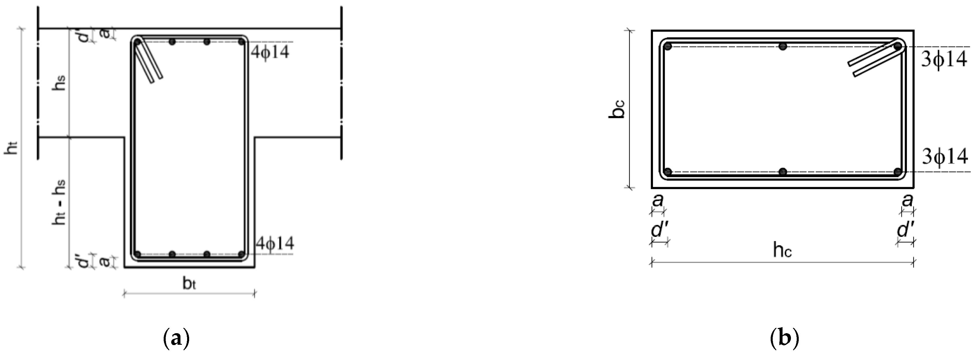
In the present study, a four bay-four storey RC frame was considered. It was ideally drawn from a residential building. The frame is characterized by a uniform bay width of 4.50 m and a story height of 3.50 m. Its members are reinforced by ϕ = 14 mm rebars. An example of a members cross section is represented in Figure 2a,b. With reference to Figure 2, for the internal columns of the first two storeys bc = 40 cm and hc = 50 cm, while in all the other cases bc = 30 cm and hc = 50 cm. Only at the top floor, the beam section is characterized by bt = 30 cm and ht = 55 cm, while in the other cases, bt = 30 cm and ht = 60 cm. The slab thickness is equal to hs = 25 cm.
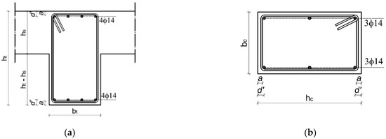
Figure 2.
Cross sections of beams (a) and columns (b).
C20/25 concrete and Aq42 rebars were implemented in the analysis with the aim of reproducing typical material properties of existing RC buildings built in the 1970s and 1980s that are supposed to be close to the end of their theoretical service life. The material properties of reinforcement were inspired by the work by Verderame et al. [33]. An equivalent water cement ratio equal to 0.60 was thought to be representative of the chemical composition of concrete. The median value of RACC,0−1 was obtained by employing the correlations reported in [27], as highlighted in Section 2.1 of the present paper.
The PSHA of reference concerns Avellino, a city located in Campania in Southern Italy. The soil class is “B”; consequently, according to Italian Code [34], the soil factor SS assumed values up to 1.20. Table 1 shows the principal variables describing the PSHA of the chosen site.

Table 1.
PSHA variables for the city of Avellino, Campania, Italy.
In the present work, the 22 ground shaking records suggested by FEMA [35], taken from “PEER Strong Motion Database Record” [36], were used, selecting only the principal component in the horizontal direction.
4.2. Material Degradation Modelling
The degradation of materials, which can be represented by a reduction in both concrete cover thickness and steel rebars area, can be easily implemented by modifying the geometric parameters of the fibre discretisation of transverse section adopted in the OpenSEES model [14]. For the sake of simplicity, a uniform degradation process was assumed on all sides of the cross section and throughout the whole element length, both for beams and columns.
The degradation models outlined in Section 2 could be employed with the aim of describing the time evolution of the nonlinear behaviour of the RC frame.
As reported in Section 2.1, the parameters controlling Equations (1)–(4) were modelled as random variables normally distributed, since their prediction is affected by both uncertainty and randomness. Consequently, it was interesting to investigate the influence on PLS of the fractiles employed in the aforementioned models.
In particular, the most important parameters controlling the degradation are the inverse effective carbonation resistance of concrete RACC,0−1 and the rate of corrosion Vcorr. The first one has a noticeable influence on the depassivation time, while the second one measures the velocity of the corrosion process.
Specifically, in the present analyses, two different scenarios were examined:
- Scenario 1: median (50%) fractiles are used to evaluate RACC,0−1 and Vcorr;
- Scenario 2: 95% fractiles are used to evaluate RACC,0−1 and Vcorr.
The second scenario represents very severe degradation conditions, when compared to the first one, dramatically reducing the depassivation time and increasing the rebar mass loss.
4.3. Parametric Field
With the aim of demonstrating the influence of carbonation-induced degradation on the seismic capacity of the structure at the global level, pushover analyses were carried out at different steps of structural age (from 0 to 50 years with steps of 10), under different environmental conditions and design cover thickness d’ (or, similarly, concrete cover a = d’ − ϕ/2). Two different scenarios for the rate of degradation were considered, as reported in the previous paragraph.
Specifically, Table 2 resumes the parametric analysis investigated. The effects of a variation of these parameters at the boundaries of the range considered in the present study are reported in the following paragraphs.
Table 2.
Parametric analysis.
The consistency of the proposed approach was demonstrated by reporting some results of analyses carried out at structural scales for the frame, evaluating the differences between the failure probability (in terms of return period) computed, neglecting the time-dependent variation of the structural response and the aforementioned equivalent constant rate and the average rate.
4.4. Application
4.4.1. Time-Evolution of Pushover Curves
In Figure 3a,b, Figure 4a,b and Figure 5a,b, a synthetic representation of the time-evolution (from 0 to 50 years) of pushover curves is presented, with the aim being to show the influence of the exposure class and the design cover on its evolution.
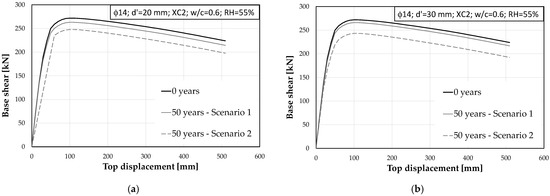
Figure 3.
Time evolution of the pushover curve for the 4 bay-4 storey RC frame (XC2, w/c = 0.60, RH = 55%) for different values of the design concrete cover d’, making use of different fractiles of the degradation model. (a) XC2, d’ = 20 mm; (b) XC2, d’ = 30 mm.
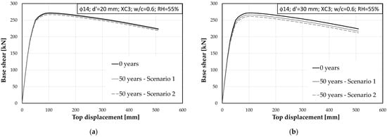
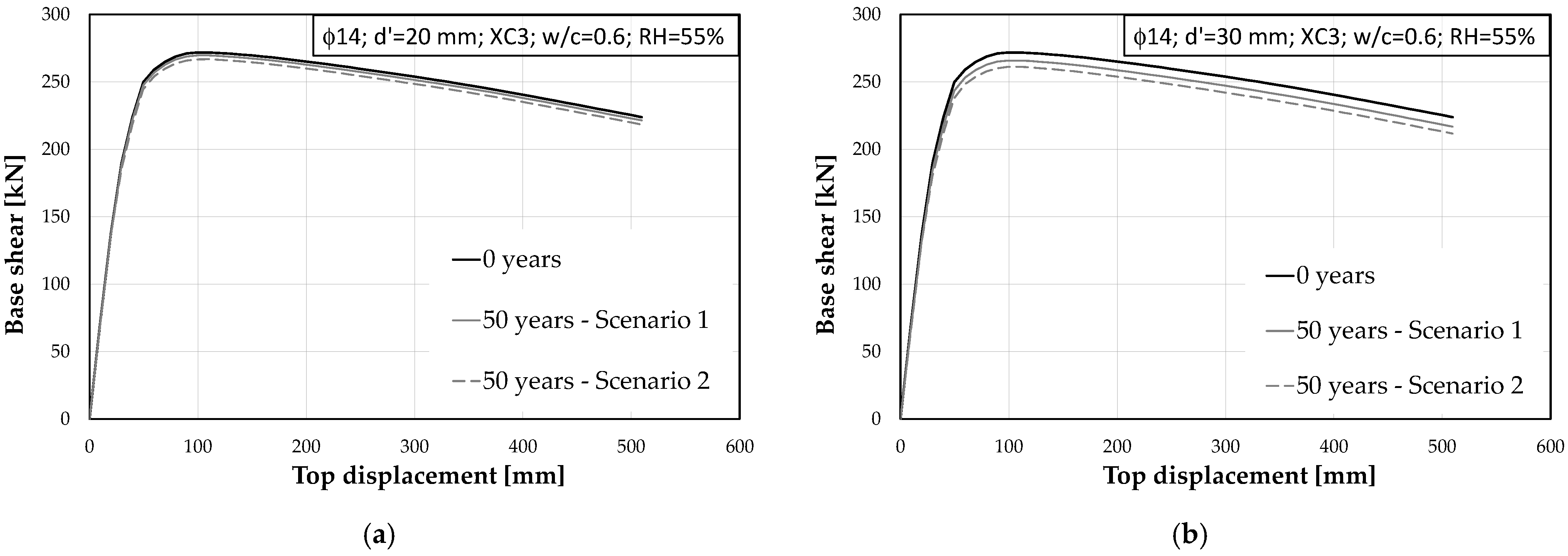
Figure 4.
Time evolution of the pushover curve for the 4 bay-4 storey RC frame (XC3, w/c = 0.60, RH = 55%) for different values of the design concrete cover d’, making use of different fractiles of the degradation model. (a) XC3, d’ = 20 mm; (b) XC3, d’ = 30 mm.
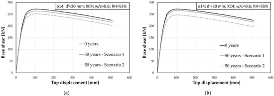
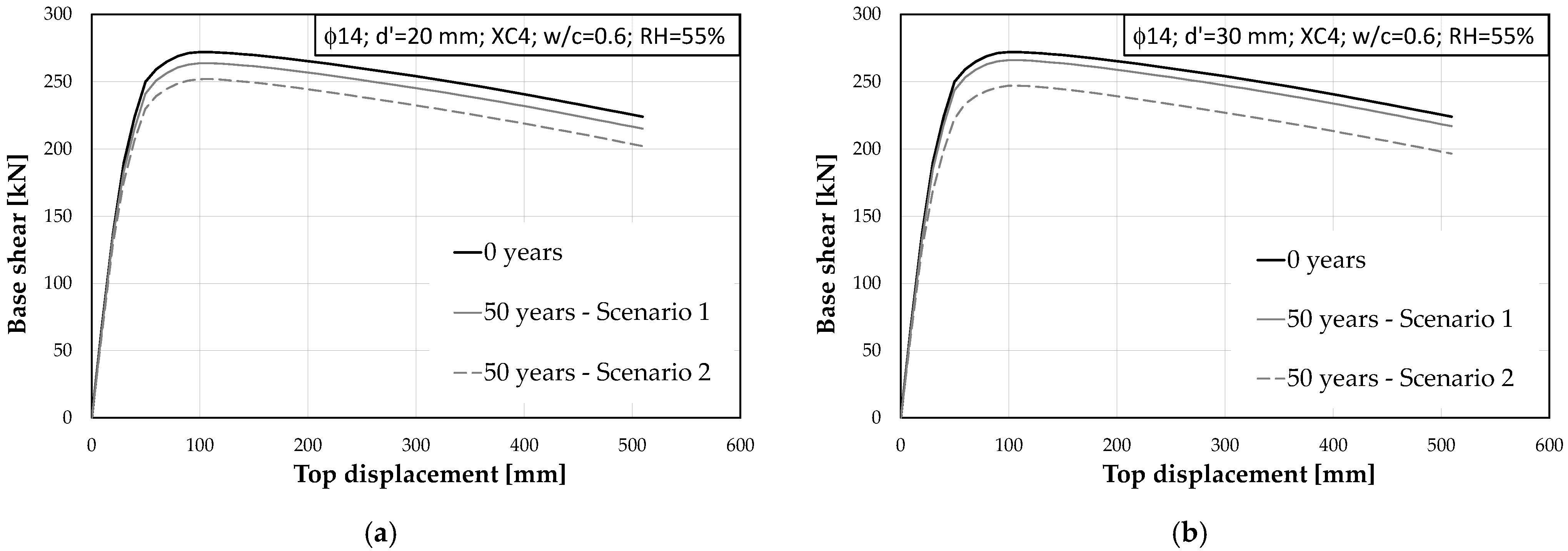
Figure 5.
Time evolution of the pushover curve for the 4 bay-4 storey RC frame (XC4, w/c = 0.60, RH = 55%) for different values of the design concrete cover d’, making use of different fractiles of the degradation model. (a) XC4, d’ = 20 mm; (b) XC4, d’ = 30 mm.
It is easy to observe that material degradation reduces the maximum base shear force; consequently, as time increases, the demand in terms of displacement increases. Nevertheless, in order to obtain consistent results, the choice of the proper values of the parameters describing degradation becomes more important, as the exposure class makes the environmental actions more severe for the structure. For instance, this choice is less relevant in the case of XC3 than in the other cases.
4.4.2. Evaluation of Median Demand and Its Dispersion
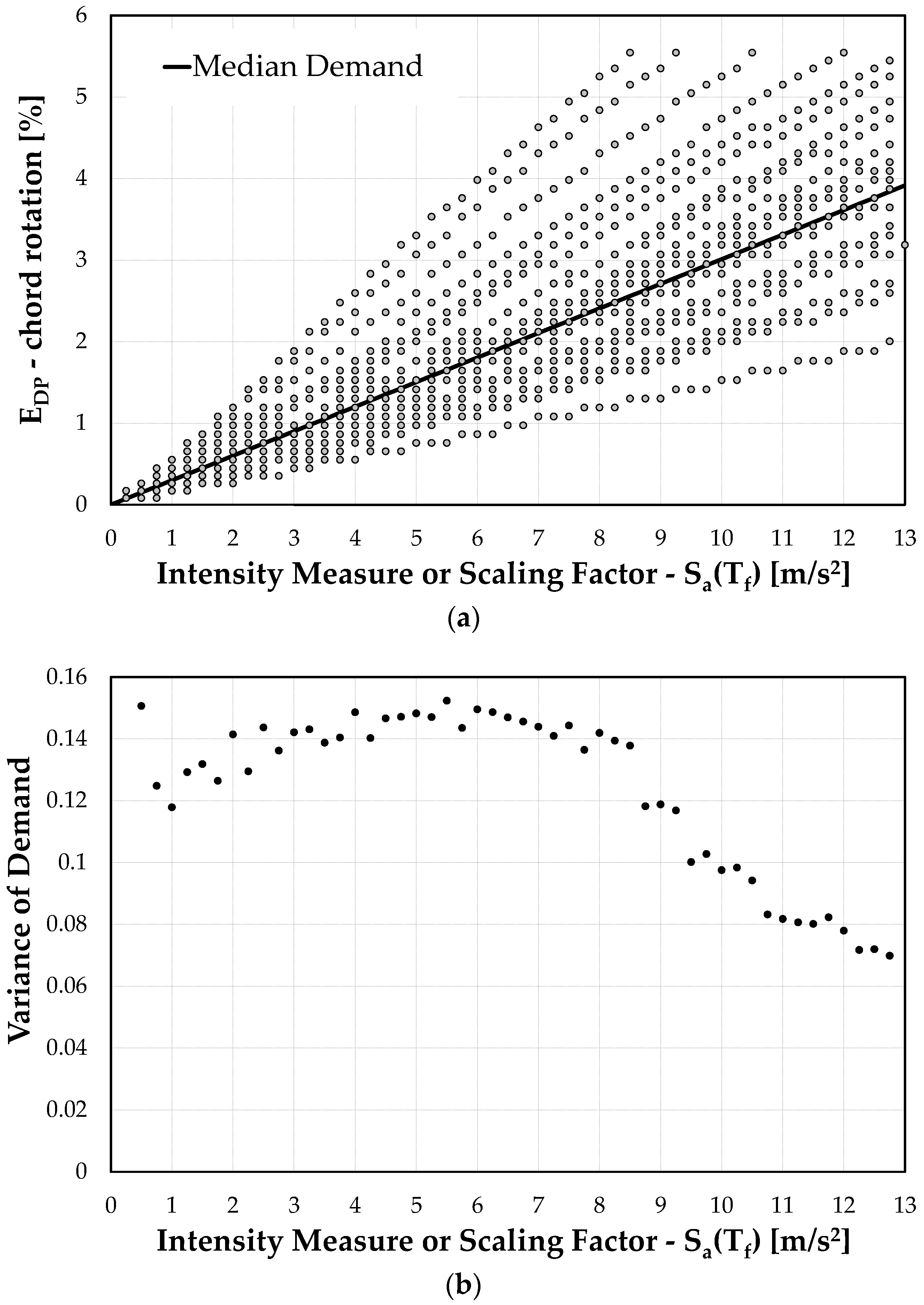
Figure 6a,b show the interpolating function—expressed by Equation (6)—representing median demand and demand dispersion for each level of SF in the case of XC2, d’ = 20 mm and time t = 50 years. Dispersion should be evaluated at each increase in scaling factor (SF), to obtain its variability with the IM.
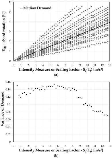
Figure 6.
Interpolation of median demand and demand variance for different values of the IM or SF in the case of XC2, d’ = 20 mm, employing 95% fractiles for RACC,0−1 and Vcorr (Scenario 2). (a) Interpolating function of median demand in the case XC2, d’ = 20 mm, time = 50 years; (b) Variance of demand in the case XC2, d’ = 20 mm, time = 50 years.
4.4.3. Evaluation of PLS
For each limit state, the intensity measure is determined by means of Equation (6), having fixed the values of the maximum chord rotation associated with each LS. Then, using Equations (6) and (10), it is possible to evaluate the PLS and the return period TR, defined as the inverse of PLS.
Table 3, Table 4, Table 5 and Table 6 resume the results obtained in the case of XC2, d’ = 20 mm at the boundary of the time span considered in the analyses.
Table 3.
Regression parameters for hazard and demand obtained at time = 0 in the case of XC2, d’ = 20 mm.
Table 4.
Results in terms of PLS obtained at time t = 0 years in the case of XC2, d’ = 20 mm.
Table 5.
Regression parameters for hazard and demand obtained at time t = 50 years in the case of XC2, d’ = 20 mm, employing 95% fractiles for RACC,0−1 and Vcorr (Scenario 2).
Table 6.
Results in terms of PLS obtained at time t = 50 years in the case of XC2, d’ = 20 mm, employing 95% fractiles for RACC,0−1 and Vcorr (Scenario 2).
4.4.4. Results of the 1st Scenario: 50% Fractiles for Evaluation of RACC,0−1 and Vcorr
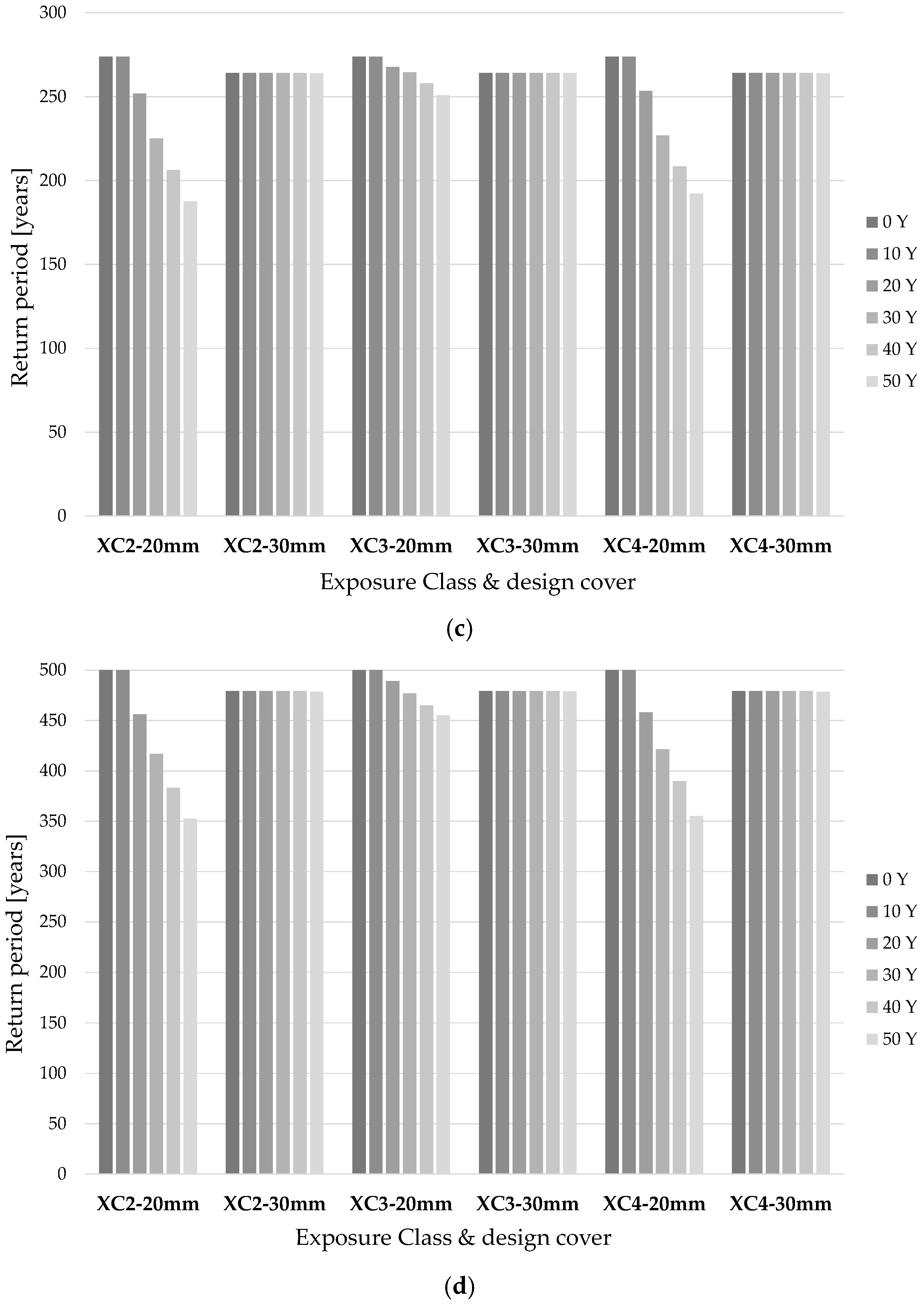
Figure 7a–d show the results of parametric analysis previously outlined in terms of return period for different limit states for the exposure classes XC3 and XC4 and for different values of the design cover (20 or 30 mm). In the degradation model, the 50% fractiles of RACC,0−1 and Vcorr are employed.

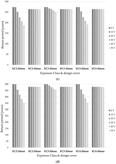
Figure 7.
Time evolution of the return period (for each LS) for the 4 bay-4 storey RC frame (w/c = 0.60, RH = 55%) for different exposure classes and different values of the design concrete cover d’, making use of median fractiles of the degradation model (Scenario 1). (a) Immediate occupancy limit state—1st scenario; (b) Damage limitation limit state—1st scenario; (c) Life safety limit state—1st scenario; (d) Collapse prevention limit state—1st scenario.
4.4.5. Results of the 2nd Scenario: 95% Fractiles for Evaluation of RACC,0−1 and Vcorr
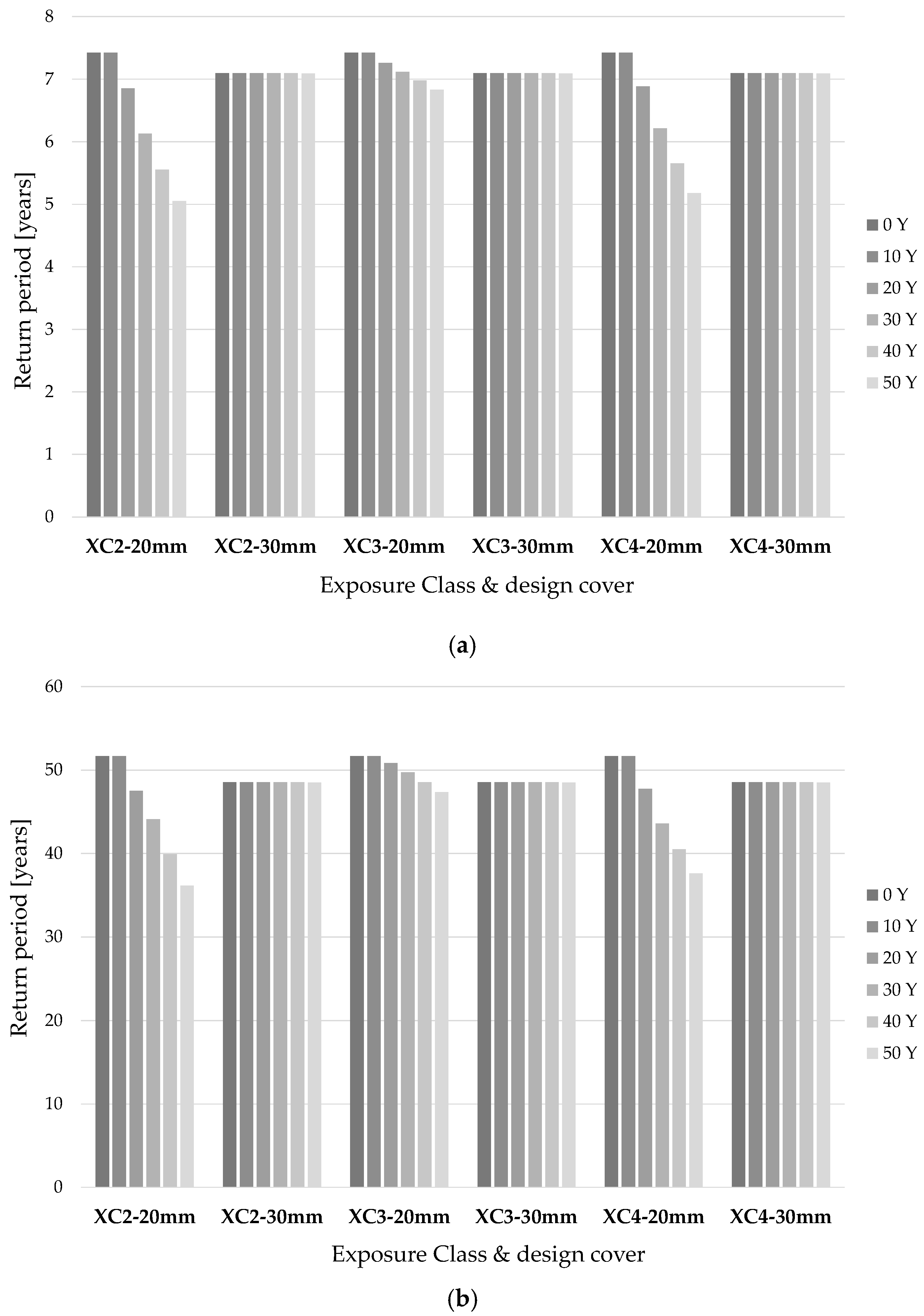
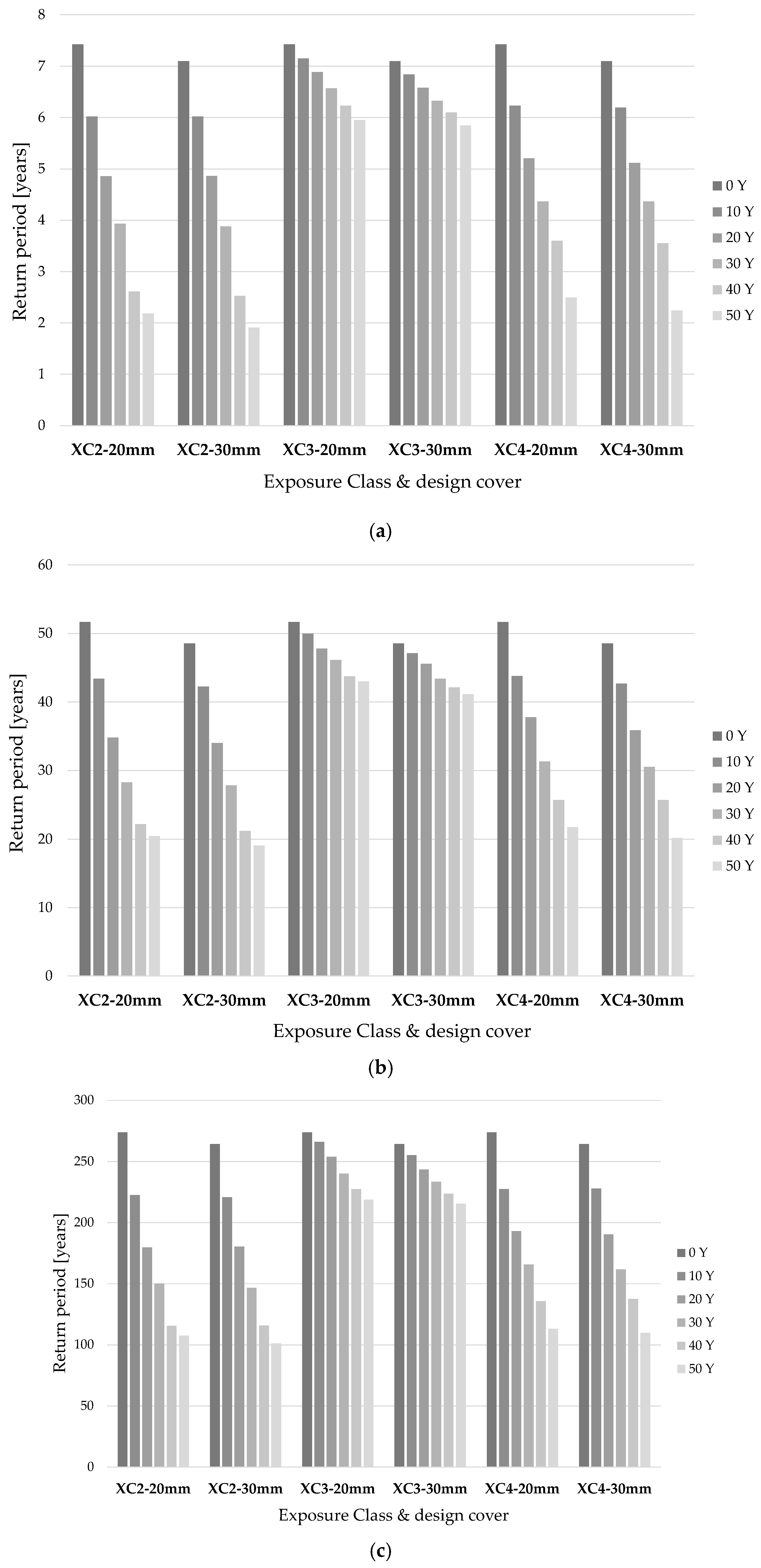
Figure 8a–d show the results of parametric analysis previously outlined in terms of the return period for different limit states for the exposure classes XC3 and XC4 and for different values of the design cover (20 or 30 mm). In the degradation model, the 95% fractiles of RACC,0−1 and Vcorr are employed.

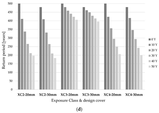
Figure 8.
Time evolution of the return period (for each LS) for the 4 bay-4 storey RC frame (w/c = 0.60, RH = 55%) for different exposure classes and different values of the design concrete cover d’, making use of 95% fractiles of the degradation model (Scenario 2). (a) Immediate occupancy limit state—2nd scenario; (b) Damage limitation limit state—2nd scenario; (c) Life safety limit state—2nd scenario; (d) Collapse prevention limit state—2nd scenario.
4.4.6. Results in Terms of Equivalent Constant Rate (ECR)
Table 7 and Table 8 report for both scenarios some comparisons between the return period “TR, 0 y”—estimated by neglecting the variation of mechanical properties due to ageing—and the return period “TR ECR”, estimated by means of Equation (12), which is able to take into account the ever-changing risk faced by the building over its design life, as formulated in [13]. The differences arising between the two and the ratios between these differences and “TR, 0 y” are shown as well.
Table 7.
Differences between TR, 0 y, TR ECR and TR, 50, employing 50% fractiles for RACC,0−1 and Vcorr (Scenario 1).
Table 8.
Differences between TR, 0 y, TR ECR and TR, 0, employing 95% fractiles for RACC,0−1 and Vcorr (Scenario 2).
Moreover, for both scenarios, the differences between the return period “TR, 0 y” and the return computed at time t = 50 years “TR, 50 y” and the ratios between these differences and “TR, 0 y” are presented.
For the sake of brevity, these return periods only deal with DL and LS limit states, since their study is very significant for common RC structures.
4.5. Discussion
In this section, the results obtained by adopting the preliminary analysis approach are presented. In order to highlight the influence of exposure class and design cover on the structural response, the risk (in terms of Return Period TR) is calculated at different stages of the theoretical structural service life Td.
Consequently, deriving an expression of the time evolution of risk, a comparison is made between the risk calculated by neglecting the effects of environmental actions TR, 0 y and the equivalent risk TRECR faced by the structure during its service life.
The principal results of this preliminary approach are summarized in the following:
- the effects of corrosion due to carbonation-induced degradation on RC members cannot be generally neglected, especially when the design cover is up to 20 mm. In these cases, a non-negligible loss in terms of the return period is observed on the structure fully exposed to XC2 and XC4 environmental actions;
- if the parameters RACC,0−1 and Vcorr are described by their median value (Scenario 1), concrete cover thickness plays a vital role in controlling the time evolution of RC sections. It can significantly delay the development of degradation, increasing the depassivation time (td) from 10 years (with a 20 mm cover) to approximately 50 years (with a 30 mm cover);
- if the parameters RACC,0−1 and Vcorr are described by their median value (Scenario 1), the usage of a design cover of 30 mm avoids significant reductions in the return period, while a design cover of up to 20 mm leads to premature degradation. This result is explained by the fact that in this condition, the depassivation time (td) is approximately equal to the theoretical service life Td; consequently, material degradation effects arise if the time span is expanded;
- the preliminary approach presented in this paper can also be employed in order to confirm the code provisions concerning the minimum values of design cover for different structural classes and exposure classes, reported in EC2 [7] confirm that in ordinary conditions (structural class S4), a design cover of 30 mm can grant a highly durable performance (in the case of carbonation induced corrosion);
- if the parameters RACC,0−1 and Vcorr are described by their median value (Scenario 1), the effect of the reduction in columns’ chord rotation capacity is still noticeable on the structure for exposure classes XC2 and XC4, when the design cover is up to 20 mm;
- if the parameters RACC,0−1 and Vcorr tend to be much higher than their median value (Scenario 2), no significant differences arise between the effect in the usage of the two values of design cover considered in this work;
- if the parameters RACC,0−1 and Vcorr tend to be much higher than their median value (Scenario 2), the effects of material degradation phenomena are still not really relevant for exposure class XC3, while they highly threaten the structural reliability for XC2 and XC4 exposure classes; indeed, in the former case, the difference between “TR, 0 y” and “TR, 50 y” is less than 20%, while in the latter cases, this difference reaches 60%;
- the variable “TRECR” is a good indicator of structural ageing. As shown in Table 7 and Table 8 (4.4.6.), if the difference between “TR, 0 y” and “TRECR” is up to 10%, the effect of ageing may be neglected, while higher values of this difference certainly imply a safety decrease (in terms of return period) higher than 25% (after 50 years);
- the decay observed in the return period is more pronounced for exposure classes XC2 and XC4 rather than for XC3, which is indeed referred to a “sheltered condition”; this is consistent with the parameters describing the degradation models reported in Section 2;
- the comparison between the two considered scenarios outlines the importance of probabilistic representation of parameters controlling Equations (1)–(4), with particular regard to RACC,0−1 and Vcorr; in the present work, they are employed in a deterministic way, although their randomness can lead to local capacity reduction that may affect the global structural response;
- since RACC,0−1 and Vcorr are defined in statistical terms, it seems evident that a more conservative approach (e.g., the usage of 95% fractiles) can lead to an excessive increase in the minimum value of design cover required to achieve a sufficiently durable performance;
- the considerations written above appear to be valid for each limit state studied.
5. Conclusions
The present paper presents a preliminary approach for practice-oriented seismic reliability analysis of RC structures affected by material degradation. Some preliminary results are also reported with the twofold aim of showing the potential of the proposed procedure and figuring out the influence of some relevant parameters (e.g., the environmental exposure class and thickness of the concrete cover) on the resulting reliability performance of a simple, yet widely representative, structure considered as a case study.
The obtained results show that:
- the effects of material degradation phenomena should be generally taken into account in the seismic reliability assessment of RC structures, if maintenance is not properly realized;
- although the work deals with the common carbonation-induced degradation phenomena that are relevant for all RC structures, the proposed procedure can be applied to any degradation phenomena, with minor specifications about material modelling and structural analysis; it is clear that carbonation-induced degradation induces a “mild” effect in terms of degradation, although it affects the entire member length, while other degradation phenomena (such as chloride ions attack) usually result in a local cross sectional strength reduction;
- the expected reduction in terms of displacement capacity induced by material degradation plays a major role in reducing the seismic reliability of the structure under consideration. As a matter of fact, the combined effect of the concrete cover loss, rebar corrosion and EDP, lim reduction can threaten the structural reliability;
- making use of simple models available in the literature for material degradation phenomena, it is possible to derive a simple expression of the time variation of the structural reliability in terms of return periods TR in a linear way; this approach may be less rigorous than the one presented in [17], but it could lead to more comprehensible results and can be more cost-effective;
- pushover analyses can be implemented for seismic reliability assessment, utilizing natural spectra (directly derived by accelerograms) in order to reproduce the record-to-record variability, as well, since the results of pushover analyses (in terms of risk) are almost equal to typical results of IDAs given in the scientific literature [16];
- the simplified procedure presented herein allows us to also explicitly predict the durability performance granted by a certain structure: for a chosen environment (in terms of exposure class), it is possible to compare the results of this analyses with the EC 8 provision for structural durability [7];
- a significant variability can be expected in the resulting structural response based on the actual rate of propagation and diffusion of the material degradation phenomena, also within the limits foreseen by the predictive models currently available in the literature and mentioned in the present paper.
Further developments of the present work will be directed towards implementing the specific aspects related to other exposure classes and expected degradation phenomena that are not included in the present paper. It will also be suitable for a comparison between the outcomes of similar analyses and the normative prescriptions for structural durability, extending the parametric field of interest.
Author Contributions
Conceptualization, E.M.; methodology, F.N. and E.M.; software, F.N., A.Z. and E.M.; validation, F.N. and E.M.; formal analysis, F.N. and E.M.; investigation, F.N. and E.M.; resources, E.M.; data curation, F.N. and A.Z.; writing—original draft preparation, F.N.; writing—review and editing, A.Z. and E.M.; visualization, F.N.; supervision, E.M.; project administration, E.M.; funding acquisition, E.M. All authors have read and agreed to the published version of the manuscript.
Funding
This research received no external funding.
Institutional Review Board Statement
Not applicable.
Informed Consent Statement
Not applicable.
Data Availability Statement
The data presented in this study are available in the article.
Conflicts of Interest
The authors declare no conflict of interest.
References
- European Commission. EU Buildings Factsheets 2013. Available online: https://ec.europa.eu/energy/eu-buildings-factsheets_en (accessed on 1 August 2021).
- Berto, L.; Vitaliani, R.; Saetta, A.; Simioni, P. Seismic assessment of existing RC structures affected by degradation phenomena. Struct. Saf. 2009, 31, 284–297. [Google Scholar] [CrossRef]
- De Schutter, G. Damage to Concrete Structures, 1st ed.; CRC Press Taylor & Francis Group: Boca Raton, FL, USA, 2013. [Google Scholar]
- Lu, C.; Jin, W.; Liu, R. Reinforcement corrosion-induced cover cracking and its time prediction for reinforced concrete structures. Corros. Sci. 2011, 53, 1337–1347. [Google Scholar] [CrossRef]
- Lay, S.; Schieβl, P. Lifecon Deliverable D 3.2, Service Life Models, “Instructions on Methodology and Application of Models for the Prediction of the Residual Service Life for Classified Environmental Loads and Types of Structures in Europe”. 2003. Available online: https://docplayer.net/49899904-Lifecon-deliverable-d-3-2-service-life-models.html (accessed on 1 September 2021).
- DuraCrete. Probabilistic Performance Based Durability Design of Concrete Structures: Statistical Quantification of the Variables in the Limit State Functions; Report No.: BE 95-1347; CUR: Amsterdam, The Netherlands, 2000. [Google Scholar]
- CEN. Eurocode 2: Design of Concrete Structures—Part 1-1: General Rules and Rules for Buildings; EN 1992-1-1:2004; Comité Européen de Normalisation: Brussels, Belgium, 2004. [Google Scholar]
- François, R.; Laurens, S.; Deby, F. Steel Corrosion in reinforced concrete. In Corrosion and its Consequences for Reinforced Concrete Structures, 1st ed.; ISTE Press Ltd.: London, UK; Elsevier Ltd.: New York, NY, USA, 2018; pp. 1–41. [Google Scholar]
- Berto, L.; Saetta, A.; Simioni, P. Structural risk assessment of corroding RC structures under seismic excitation. Constr. Build. Mater. 2012, 30, 803–813. [Google Scholar] [CrossRef]
- Kashani, M.M.; Lowes, L.N.; Crewe, A.J.; Alexander, N.A. Phenomenological hysteretic model for corroded reinforcing bars including inelastic buckling and low-cycle fatigue degradation. Comput. Struct. 2015, 156, 58–71. [Google Scholar] [CrossRef] [Green Version]
- Vecchi, F.; Belletti, B. Capacity Assessment of Existing RC Columns. Buildings 2021, 11, 161. [Google Scholar] [CrossRef]
- Erduran, E.; Martinelli, E. Some remarks on the seismic assessment of RC frames affected by carbonation-induced corrosion of steel bars. In Proceedings of the fib CACRCS DAYS 2020: Capacity Assessment of Corroded Reinforced Concrete Structures, on-line event, 1–4 December 2020. [Google Scholar]
- Sohail, M.G.; Kahraman, R.; Ozerkan, N.G.; Alnuaimi, N.A.; Gencturk, B.; Dawood, M.; Belarbi, A. Reinforced Concrete Degradation in the Harsh Climates of the Arabian Gulf: Field Study on 30-to-50-Year-Old Structures. J. Perform. Constr. Fac. 2018, 32, 04018059. [Google Scholar] [CrossRef]
- Mazzoni, S.; McKenna, F.; Scott, M.H.; Fenves, G.L. Open System for Earthquake Engineering Simulation User Command-Language Manual. 2009. Available online: https://OpenSEES.berkeley.edu/OpenSEES/manuals/usermanual/index.html (accessed on 1 September 2021).
- Pinto, P.E.; Giannini, R.; Franchin, P. Specialized methods for seismic problems. In Seismic Reliability Analysis of Structures, 1st ed.; IUSS Press: Pavia, Italy, 2004; pp. 215–218. [Google Scholar]
- Cornell, C.A.; Jalayer, F.; Hamburger, R.O.; Foutch, D.A. Probabilistic basis for 2000 SAC Federal Emergency Management Agency Steel Moment Frame Guidelines. ASCE J. Struct. Eng. 2002, 128, 526–533. [Google Scholar] [CrossRef] [Green Version]
- Vamvatsikos, D.; Dolšek, M. Equivalent constant rates for performance-based seismic assessment of ageing structures. Struct. Saf. 2011, 33, 8–18. [Google Scholar] [CrossRef]
- Vamvatsikos, D.; Cornell, A.C. Incremental Dynamic Analysis. Earthq. Eng. Struct. D 2002, 31, 491–514. [Google Scholar] [CrossRef]
- Fajfar, P. Capacity Spectrum Method Based on Inelastic Demand Spectra. Earthq. Eng. Struct. D 1999, 28, 979–993. [Google Scholar] [CrossRef]
- Dolsek, M.; Fajfar, P. IN2—A Simple Alternative for IDA. In Proceedings of the 13th World Conference on Earthquake Engineering, Vancouver, BC, Canada, 1–6 August 2004. Paper No. 3353. [Google Scholar]
- Faella, C.; Lima, C.; Martinelli, E. Non-linear static methods for seismic fragility analysis and reliability evaluation of existing structures. In Proceedings of the 14th World Conference on Earthquake Engineering, Beijing, China, 12–17 October 2008. [Google Scholar]
- CNR-DT 212/2013. Recommendations for the Probabilistic Seismic Assessment of Existing Buildings; Consiglio Nazionale delle Ricerche: Rome, Italy, 2013; Available online: http://www.cnr.it/sitocnr/IlCNR/Attivita/NormazioneeCertificazione/DT212.html (accessed on 1 September 2021). (In Italian)
- Lima, C.; Martinelli, E. OpenSEES procedure for implementing reliability analysis of RC frames. In Proceedings of the OpenSEES Days, 2nd Italian Conference, Salerno, Italy, 10–11 June 2015. [Google Scholar]
- FIB. Model Code for Service Life Design; Fédération Internationale du Béton: Lausanne, Switzerland, 2006. [Google Scholar]
- FIB. Model Code for Concrete Structures 2010; Fédération Internationale du Béton: Lausanne, Switzerland, 2013. [Google Scholar]
- Tuutti, K. Corrosion of Steel in Concrete; Swedish Cement and Concrete Research Institute: Stockholm, Sweden, 1982. [Google Scholar]
- DARTS. Durable and Reliable Tunnel Structures: Data, European Commission, Growths 2000, Contract G1RD-CT-2000-00467; Project GrD1-25633; Comité Européen de Normalisation: Brussels, Belgium, 2004. [Google Scholar]
- Siemes, T.; Edvardsen, C. DURACRETE: Service Life Design for Concrete Structures. 1999, pp. 1343–1356. Available online: https://www.irbnet.de/daten/iconda/CIB2068.pdf (accessed on 1 September 2021).
- Faella, C.; Lima, C.; Martinelli, E.; Nigro, E. Comparative Application of Capacity Models for Seismic Vulnerability Evaluation of Existing RC Structures. In Proceedings of the MERCEA’08 Conference, Reggio Calabria, Italy, 8–11 July 2008; pp. 1187–1194. [Google Scholar]
- Kunnath, S.K.; Reinhorn, A.M.; Park, Y.J. Analytical modeling of inelastic seismic response of R/C structures. J. Struct. Eng. 1990, 116, 996–1017. [Google Scholar] [CrossRef]
- Spacone, E.; Filippou, F.C.; Taucer, F.F. Fiber beam-column model for nonlinear analysis of R/C frames. 1: Formulation. Earthq. Eng. Struct. D 1996, 25, 711–725. [Google Scholar] [CrossRef]
- Newmark, N.M.; Hall, W.J. Earthquake Spectra and Design; Earthquake Engineering Research Institute: Berkeley, CA, USA, 1982. [Google Scholar]
- Verderame, G.M.; Ricci, P.; Esposito, M.; Sansiviero, F.C. Le caratteristiche meccaniche degli acciai impiegati nelle strutture in c.a. realizzate dal 1950 al 1980. In Proceedings of the XXVI Convegno Nazionale AICAP “Le Prospettive di Sviluppo delle Opere in Calcestruzzo Strutturale nel Terzo Millennio”, Padova, Italy, 19–21 May 2011. Paper No. 54. [Google Scholar]
- DM 17/01/2018. Italian Technical Code of Constructions; Ministerial Decree: Rome, Italy, 2018. [Google Scholar]
- Federal Emergency Management Agency (FEMA). Quantification of Building Seismic Performance Factors; CreateSpace Independent Publishing Platform: Scotts Valley, CA, USA, 2009. [Google Scholar]
- Pacific Earthquake Engineering Research Center (PEER NGA DATABASE). Available online: http://peer.berkeley.edu/nga (accessed on 1 September 2021).


Publisher’s Note: MDPI stays neutral with regard to jurisdictional claims in published maps and institutional affiliations. |
© 2021 by the authors. Licensee MDPI, Basel, Switzerland. This article is an open access article distributed under the terms and conditions of the Creative Commons Attribution (CC BY) license (https://creativecommons.org/licenses/by/4.0/).