Article

Resilient Anomaly Detection in Fiber-Optic Networks: A Machine Learning Framework for Multi-Threat Identification Using State-of-Polarization Monitoring

by
Gulmina Malik
1,*,
Imran Chowdhury Dipto
1,
Muhammad Umar Masood
1,
Mashboob Cheruvakkadu Mohamed
1,
Stefano Straullu
2,
Sai Kishore Bhyri
3,
Gabriele Maria Galimberti
4,
Antonio Napoli
5,
João Pedro
6,
Walid Wakim
7 and
Vittorio Curri
1
1
Department of Electronics and Telecommunications, Polytechnic University of Turin, 10129 Turin, Italy
2
LINKS Foundation, 10129 Turin, Italy
3
Optical Networks, Nokia, Bangalore 560045, India
4
Optical Networks, Nokia, 20060 Milan, Italy
5
Optical Networks, Nokia, 81541 Munich, Germany
6
Optical Networks, Nokia, 2720-092 Carnaxide, Portugal
7
Optical Networks, Nokia, Naperville, IL 60563, USA
*
Author to whom correspondence should be addressed.
AI 2025, 6(7), 131; https://doi.org/10.3390/ai6070131
Submission received: 16 May 2025 / Revised: 9 June 2025 / Accepted: 13 June 2025 / Published: 20 June 2025
(This article belongs to the Special Issue Artificial Intelligence in Optical Communication Networks)

Abstract

We present a thorough machine-learning framework based on real-time state-of-polarization (SOP) monitoring for robust anomaly identification in optical fiber networks. We exploit SOP data under three different threat scenarios: (i) malicious or critical vibration events, (ii) overlapping mechanical disturbances, and (iii) malicious fiber tapping (eavesdropping). We used various supervised machine learning techniques like k-Nearest Neighbor (k-NN), random forest, extreme gradient boosting (XGBoost), and decision trees to classify different vibration events. We also assessed the framework’s resilience to background interference by superimposing sinusoidal noise at different frequencies and examining its effects on the polarization signatures. This analysis provides insight into how subsurface installations, subject to ambient vibrations, affect detection fidelity. This highlights the sensitivity to which external interference affects polarization fingerprints. Crucially, it demonstrates the system’s capacity to discern and alert on malicious vibration events even in the presence of environmental noise. However, we focus on the necessity of noise-mitigation techniques in real-world implementations while providing a potent, real-time mechanism for multi-threat recognition in the fiber networks.

1. Introduction

Optical networks serve as the critical infrastructure for enabling ultra-high-speed and high-capacity data transmission in contemporary telecommunication systems. The exponential surge in internet traffic, emerging 6G applications, and rising demand for high-bandwidth services necessitates the optimization of optical network performance and reliability [1]. Optical communication systems transmit exceptionally large volumes of data, including sensitive and confidential information, across long distances. As such, ensuring the integrity and reliability of data transmission is of paramount importance in maintaining secure and trustworthy communication infrastructures [2]. The use of pre-installed optical fiber infrastructures for environmental monitoring has garnered more attention in recent years due to the extensive deployment of optical fiber networks in both terrestrial and subsea scenarios [3,4,5].
Fiber-optic cables are intrinsically sensitive to environmental conditions like temperature, mechanical stress, and vibrations [6,7]. Distributed acoustic sensing (DAS) systems can detect dynamic events such as mechanical vibrations up to the kilohertz range, and are widely used for earthquake detection [8,9] and metropolitan monitoring [10,11]. As we know, optical fiber networks form the backbone of global connectivity, linking billions of users worldwide. Their indispensable function and inherent sensitivity, however, render them susceptible to a range of impairments, including fiber breaks, targeted physical tampering, unauthorized eavesdropping via fiber bending, and ambient mechanical vibrations [12,13]. Such perturbations can degrade the propagating optical signal, leading to severe network impairments, widespread service outages, and breaches of data confidentiality. To provide early warnings for situations that endanger the health of optical fiber networks, monitoring the metropolitan environment is very essential. It is also critical to classify and localize the fiber anomalies and limit their impact by taking preventive measures proactively. Numerous studies have addressed the classification and localization of fiber anomalies; for instance, [14] utilized optical time-domain reflectometry (OTDR) trace analysis to detect and pinpoint disruptive events. In contrast, monitoring the state of polarization (SOP) offers greater sensitivity to subtle physical perturbations, as it directly captures alterations in the polarization state of light propagating through the fiber and can discriminate the type of anomaly. The study in [15] employs the angular speed of SOP (SOPAS) compared to a predetermined threshold to identify fiber impairments such as bending, shaking, or minor impact and other external disturbances. Meanwhile, the authors of [16] use transfer learning on SOP-derived data, while in [17], they investigate computer vision methodologies, transforming polarization measurements into visual formats or images to classify threats in optical networks.
Recent advancements in machine learning (ML) methodologies demonstrate significant promise in addressing the challenges of fiber event detection and localization [18]. Deep learning (DL) offers a powerful solution by learning complex patterns in high-dimensional SOP data. In order to identify and locate fiber disruption in optical networks, recent research has used supervised and unsupervised deep learning. Detection and localization of reflective fiber events caused by connectors or splices, multi-task long short-term memory (LSTM), and convolutional neural networks (CNNs) (first proposed in [19]) have been suggested in [20,21], providing precise detection and location even at low signal to noise ratio (SNR). The study in [22] introduced a one-dimensional neural network (1D-CNN) for the identification of adversarial events in a noisy environment. In [14], an autoencoder is employed to detect anomalies in optical fibers, followed by an attention-based bidirectional gated recurrent unit (BiGRU) architecture to classify and accurately localize the events. The work in [23] uses the data clustering module (DCM) to analyze the patterns of the monitoring data and the convolutional autoencoder to extract features and clustering to locate the location.
Contemporary deep learning techniques employ neural networks for anomaly detection due to their significantly reduced inference time [24], compared to classic ML models; however, they necessitate a substantial amount of data and computational resources to achieve an acceptable level of accuracy. However, for our study, supervised classical ML methods provided efficient and practical solutions due to their low processing costs and reduced need for high-dimensional feature space.
Despite these advances, a cohesive and resilient framework for real-time SOP-based multi-threat detection remains underexplored. While prior work in [25,26,27] has used ML to detect eavesdropping and harmful vibration events in real fiber installations, our study proposes a machine learning-based framework that takes advantage of the angular speed and temporal evolution of SOP (SOPAS) to detect and classify multiple fiber anomalies, including malicious vibrations, overlapping physical disturbances, and fiber tapping events. Unlike previous research, we evaluate the robustness of this model by introducing synthetic noise (e.g., sinusoidal) to emulate real-world environmental interference and assess the classifier’s ability to distinguish between benign and malicious anomalies. Our key objective is to create a lightweight yet resilient SOP-based monitoring architecture that can trigger alerts or initiate rerouting protocols based on the severity of the detected anomaly, thus improving the self-healing and defensive capabilities of optical networks. This work builds upon and extends our previous contributions in the field [28,29,30], aiming to bridge the gap between experimental SOP monitoring and deployable anomaly detection systems.

2. State of Polarization (SOP) as a Sensing Mechanism

The SOP serves as a highly sensitive, real-time sensing mechanism for detecting mechanical disturbances in optical fiber networks. The orientation of the electric field as it traverses the fiber is referred to as the polarization state. Optical fiber sensors exhibit polarization sensitivity and are typically prone to polarization fading [31]. Monitoring the polarization state trajectory on the Poincaré sphere allows SOP analysis to detect minute birefringence shifts caused by temperature changes, traffic, and external mechanical disturbances (e.g., drilling vibrations). In laboratory experiments, polarimeters coupled with programmable vibration sources (typically 1–10 Hz) provide high-fidelity measurement of the stokes parameters. Each SOP recording consists of numerous variables, incorporating the temporal variation of stokes parameters [32]. Fluctuations in SOP may signify fiber fluctuations. Early detection of fiber damage or anomalies is made possible by monitoring these fluctuations. There are four stokes parameters ( S 0 , S 1 , S 2 , and S 3 ) which characterize the polarization state of electromagnetic waves, or light. S 0 represents the total intensity or power of the optical beam or light while the other three components, S 1 , S 2 , and S 3 , are coordinate values in the coordinate system that a Poincaré sphere represents. S 1 is the difference in intensity between horizontally and vertically polarized light. S 2 is the difference in intensity between the diagonal (45°) and anti-diagonal (−45°). And S 3 represents the difference in intensity between left and right circular polarized components [33]. Any perfect polarization can be expressed as a point on the Poincaré sphere [5].
The time variation of the stokes parameters’ speed on the Poincar’e sphere at a specific angle is defined by SOPAS [34]. The formula is given by
ω [ k ] = arccos S k · S k 1 S k   S k 1 · 1 T s
where the sample period is denoted by T s . The dot product of the stokes vectors at time k and time k 1 is represented by ( S k · S k 1 ) , which indicates the extent to which these two vectors point in the same direction. The magnitude of the two stokes vectors is represented by the denominator.
To quantify the rate of change of the polarization orientation between successive stokes vectors S k 1 and S k throughout the sampling period T s , the SOP angular speed, represented by the symbol ω [ k ] , uses units of rad / s . The ratio of polarized to total light intensity in the fiber is known as the degree of polarization (DOP), and it is always 1. The strength of vibration is correlated with the SOPAS.
Polarization controllers are used to establish a desired polarization state in polarization-managed sensing networks. Standard optical fibers, on the other hand, cannot maintain this condition, leading to unexpected polarization at any point along the fiber instead of user-defined values [35]. However, SOP measurements in real-world installations have to deal with noise sources such as scattered ambient light, normalization problems in telemetry interfaces.
In this paper, we investigate the use of optical fiber as a sensing medium and present three distinct scenarios involving anomaly detection through the analysis of the SOP data obtained from a polarimeter. Machine learning techniques are used to classify these anomalies, which may indicate potential threats to network integrity. The identified scenarios are detailed in the following subsections. The experimental setup for the vibration generation is discussed in Section 3. Section 4 outlines the machine learning architecture implemented for vibration detection. In Section 5, we evaluate the model’s performance under varying vibration intensities and in the presence of additive noise, followed by a comparative analysis. The study concludes with key findings summarized in Section 6.

2.1. Eavesdropping

An adversary, known as a hacker, could compromise the physical layer of the telecommunications system to intercept private information and harm vendors. Fiber tapping is the predominant technique among the numerous fiber-tampering methods identified [36]. It involves macro-bending the fiber cable at a low curvature radius to compromise the total internal reflection condition that permits light propagation. The light then leaks from the fiber at the bending point, where it can be intercepted by an eavesdropping device. The communication system may undergo a minor power reduction [37,38] and a bending-induced change in SOP [39], both of which can be detected by an SOP detection system.
To replicate this phenomenon, we employed a commercial optical fiber identification (OFI) device that secures and significantly bends the fiber linked to a 13 km metropolitan cable [40]. A handgrip, when tightened, bends the internal fiber of the instrument to control clamping. Eavesdropping occurs when the equipment detects light leaking. Furthermore, it denotes the trajectory of the light leak, facilitating a hacker’s ability to extract data from the leaking light.
Figure 1 illustrates how bending has an adverse impact on the stokes parameters. Initial experiments were conducted with OFI securely fastened to the optical bench, separating it from outside influences, in order to describe the signature that the macro-bends had on the SOP. After 30 s of gentle clamping, the fiber was released. The S 0 component records the instantaneous power, and the polarimeter outputs the whole stokes vector. The outcomes of six tests are illustrated in Figure 1, where the behavior of the stokes parameters is evident for a clamp held for approximately 10 s. The instantaneous power gradually changes between levels over a period of about 1 s when the clamp is closed, exhibiting a sudden spike, respectively. The eavesdropping tests were repeated approximately 50 times to provide a more thorough understanding of the stokes parameters’ response.
We also computed the SOPAS deviation according to Equation (1). The higher peaks of the angular speed mean the parts when the clamp is closed, with the highest angular speed being 2.5 radians per second. In a real-world scenario, a malicious hacker would likely manipulate the optical fiber before connecting it to the device, rather than placing it firmly on a surface. In addition, the device would typically remain attached to the cable for several hours to maximize data intercept. These SOPAS and their temporal derivatives are integrated as key features for vibration event classification in our ML approach (Section 2.3).

2.2. Simultaneous Events

We also examined how polarization signatures appear when two disruptive events occur simultaneously. Every disrupting event has a distinct polarization signature. We generated several signatures to monitor the polarization state change on the Poincar’e sphere. These signatures were synthesized to capture the dynamic evolution of the polarization state.
Intentional or construction-site fiber shaking, as well as tapping (eavesdropping) into the fiber to leak private and sensitive information, is considered a hostile incursion that can mislead network operators. A sophisticated ML model is needed in these situations so that it can identify and distinguish between the events and notify the service providers. Identification is made more difficult by these overlapping disturbances, which calls for more advanced detection methods.
In this section, we investigated the use of ML-driven SOP analysis for the detection of overlapping anomalies in optical networks. Utilizing XGBoost [41], our model accurately classified overlapping fiber anomalies, which are further discussed in [30]. The results demonstrated that, for proactive network maintenance and enhanced fiber infrastructure security, ML is more accurate and dependable than traditional fault detection techniques.
For this experiment, we used a robotic arm that uses a frequency of 3 Hz and an angle of deviation 90° to move the fiber up and down for shaking. We manually tapped the fiber once every second to hit it. Because each event generates a unique polarization signature, we captured them using the stokes parameters, as shown in Figure 2. The pronounced peaks in these traces correspond to the physical tapping (fiber hits). However, the robotic arm’s coordinated action of shaking the fiber and hitting it was synchronized for the creation of overlapping events.
Following the collection of this data, we carried a few pre-processing procedures, and then fed the dataset into our model. The results, discussed in [30], concluded that XGBoost achieved higher accuracy than the other classifiers, as it effectively captured non-linear patterns and is computationally efficient. Therefore, it was chosen for further analysis. The model accurately predicted the data with an accuracy of 98%, and only misclassified 2.06% of overlap events.
This ML model enables real-time identification of multiple threat scenarios by effectively differentiating between benign vibrations and deliberate intrusions (e.g., tapping), owing to its training on overlapping tampering events and noise-augmented datasets. It provides a robust framework for enhancing network resilience against complex and evolving fault conditions.

2.3. State-of-Polarization-Based Vibration Monitoring

In this section, we will describe the complete architecture of the vibration monitoring system and the experimental setup through which the dataset was collected.
In Figure 3, we can observe the different levels of shaking and their corresponding signatures as represented by the stoke parameters. As the shaking increases, the range of variation in the stokes parameters decreases. In the noise-free data shown in Figure 3, for 10 Hz shaking, the value of S 3 component oscillates between 0.25 and 0.45, whereas it spans a wider range of 0.15–0.65 under 3 Hz excitation.
Upon introducing varying noise levels into the dataset, the polarization signatures, corresponding to each shaking frequency, exhibited noticeable shifts. For instance, Figure 4 illustrates a comparative analysis of the stokes parameter trajectories between the clean dataset and the dataset contaminated with 3 Hz noise, highlighting the distortion introduced by external perturbations. To gain a more granular understanding, each stokes parameter was individually analyzed in the figure to clearly visualize the impact and shift caused by the 3 Hz noise. The dotted lines indicate the fingerprints affected by added noise, while the solid lines represent the original, unaltered fingerprints.

3. Vibration Emulation and State-of-Polarization Sensing Setup

Each event produces a distinct polarization signature. To study these, we generated multiple signatures by tracking changes in the polarization state on the Poincaré sphere using stokes parameters. We used an Arduino-controlled robotic arm to generate the shaking of various frequencies. These events are explained in Table 1, where those that do not affect the fiber’s integrity are classified as “No event”. “Shaking (1 Hz)” are the ones that function as ambient sound and have a lower level of severity. “Shaking (3 Hz)” are moderately sensitive and can cause mild disturbances in the metropolitan fiber. Nonetheless, “Shaking (5 Hz) and Shaking (10 Hz)” are more sensitive to fiber integrity and require countermeasures. The vibration generation testbed is detailed in our earlier study [29]. A continuous-wave laser source emitting light at 1530 nm with 6 dBm power is launched into the sensing fiber. The testbed includes two segments of single-mode fiber (SMF), 8 km and 5 km in length, connected to an SMF section manipulated by the robotic arm. The Arduino-based arm is integrated into a custom-printed circuit board (PCB) along with its driver board and Arduino UNO R3 for improved stability. At the receiving end, an additional fiber spool is connected to a Novoptel PM1000 polarimeter, which captures the temporal evolution of stokes parameters to discern polarization fingerprints.
We set the sampling at 1500 samples per second. The averaging time exponent (ATE) is set to 16. The polarimeter analyzes the orientation of light scattered on the Poincaré sphere. SOPAS evaluations are generated by extrapolating the polarization state changes caused by the robotic arm. We recorded unique polarization signatures of vibrations, as outlined in the previous section, to differentiate between critical intensity levels. The experiments conducted by the robotic arm generated SOP and SOPAS data corresponding to each vibration level, which were subsequently utilized to train and evaluate our ML model.

4. Machine Learning Model Architecture

The machine learning architecture proposed in this study is purposefully designed to detect and classify mechanical anomalies in optical fiber networks by analyzing the temporal evolution of polarization states. The input data consist of time-series measurements of the stokes parameters and corresponding angular speed, sampled at a frequency of 1500 samples per second. This fine-grained temporal resolution enables the system to capture minute polarization fluctuations indicative of vibrational disturbances or external intrusions.
The input features taken for the training of the model were the stokes parameters ( S 1 , S 2 , and S 3 ) and the SOPAS, and the dataset consists of the target column named “Label” with values corresponding to different classes. These were the features used to train the ML classifiers in this experiment. After identifying the ideal model, it was then tested on the unseen data with various noise levels. After saving and testing the ideal model on the datasets with noise, it was noticed that further enhancements to these features were necessary for that model to perform better on the datasets with varying noise levels. In addition to the input features, we have added rolling mean and standard deviation of the input features ( S 1 , S 2 , and S 3 , SOPAS), with window sizes of 500 and 1000. We first ran the experiment with 500 as the window size and then tried with 1000. Following the addition of both 500 and 1000, empirical evaluation revealed enhanced performance of the model when assessed on unseen data. Similarly, we tested incorporating lag features of the input variables and discovered that the model exhibits improved performance when these lag features are included up to the third order, therefore successfully capturing short-term temporal dependencies.
To enhance the model’s ability to capture temporal dynamics, the raw polarization data are transformed into a higher-dimensional feature representation. This is achieved by incorporating temporally shifted (lagged) instances of each stokes parameter and the SOPAS up to third order, thereby enabling the model to learn from recent temporal patterns and transitional behavior. In parallel, rolling statistical descriptors, including localized means and standard deviations, are computed over sliding windows to extract trend sensitive features while attenuating transient noise and fluctuations.
Each data instance is associated with a class label corresponding to the severity of the induced mechanical disturbance: No Event, Shaking at 1 Hz, 3 Hz, 5 Hz, or 10 Hz. The dataset is partitioned into training and testing sets using a conventional 80:20 split. This structured representation enables the application of supervised learning methods capable of identifying complex patterns in both clean and noisy environments. Table 2 is a summary of the features considered for training the models on the clean dataset before they were tested on the unseen datasets. To identify trends and stability, rolling statistics such as mean ( m 2 , m 3 ) and standard deviation ( m 4 , m 5 ) are computed over two sliding windows, enabling the model to discern additional patterns for each window feature. Additionally, lag features ( m 6 , m 7 , m 8 ) are used to assist the model in identifying temporal dependencies.
The resulting architecture is structured to support efficient training and inference, with a moderate computational footprint and compatibility with a range of classification models. Figure 5 illustrates the complete machine learning framework, including the training process, classifier integration, and real-time event classification. The flowchart outlines key steps such as data pre-processing, feature extraction, model training, and classification of new SOP data. After training, the classifier is used to assess the severity of unseen polarization events and generate alerts accordingly, enabling timely response to potential fiber anomalies. The subsequent section presents the supervised learning models evaluated within this framework, detailing their implementation, configuration parameters, and comparative performance.

4.1. Machine Learning Classifiers

To find the best classifier for our malicious vibrations classification task, we thoroughly examined a number of supervised machine learning techniques. We have chosen different classifiers from the Scikit-Learn package according to their performance metrics, utility, and effective predictability. We employed k-nearest neighbor (k-NN), decision trees, random forest (RF), and extreme gradient boosting (XGBoost) in our investigation, which are explained in detail below.
RF is a powerful supervised learning algorithm designed for both classification and regression problems. It operates by constructing an ensemble of decision trees, each trained on a randomly sampled subset of the training data through a bootstrap aggregation (bagging) process. In this study, we employed a forest consisting of 100 decision trees, each with a maximum depth limited to 6, to control model complexity and reduce the risk of overfitting. RF improves predictive performance by averaging the outputs of individual trees, which enhances generalization and mitigates variance. Additionally, it leverages dimensionality reduction and parallel computation, enabling faster training and more robust handling of high-dimensional data and noise [42].
The k-NN classifier assigns unlabeled data points to the class of the most similar labeled instances based on their proximity in the feature space [43]. The labels of the K-nearest patterns in the data space serve as the foundation for nearest neighbor techniques. Since it establishes how many neighbors to take into account while making predictions, the value of k is crucial in k-NN. A greater k can assist in smoothing out the predictions and lessening the impact of noisy data if the dataset contains significant outliers or noise. We selected the value of K to be in the range [5, 50] to ensure robust classification performance across varying data distributions.
Decision trees are a supervised classification technique that uses a tree-like decision model that depends on the dataset values [44]. A decision tree solves the problem by using the tree representation, where each leaf node represents a class label and the internal nodes of the tree represent the features. The decision tree can be used to represent any Boolean function on discrete attributes. We kept the depth of tree in our model to [3, 5, 10, 15, 20], to reduce overfitting.
XGBoost is an ensemble learning method that integrates predictions from numerous weak models for a more robust prediction. It uses a classification and regression tree (CART) as its primary learning [41]. It is also compatible with parallel processing, allowing one to train models on large datasets in a practical time frame. We have trained 150 decision trees with a learning rate of 0.4.

4.2. Evaluation Metrics

To evaluate the performance of our model, we used standard metrics derived from the confusion matrix namely: accuracy, precision, recall, and F-1 score. These metrics help quantify how well the model distinguishes between different event types, including No Event, Shaking—1 Hz, Shaking—3 Hz, Shaking—5 Hz, and Shaking—10 Hz.

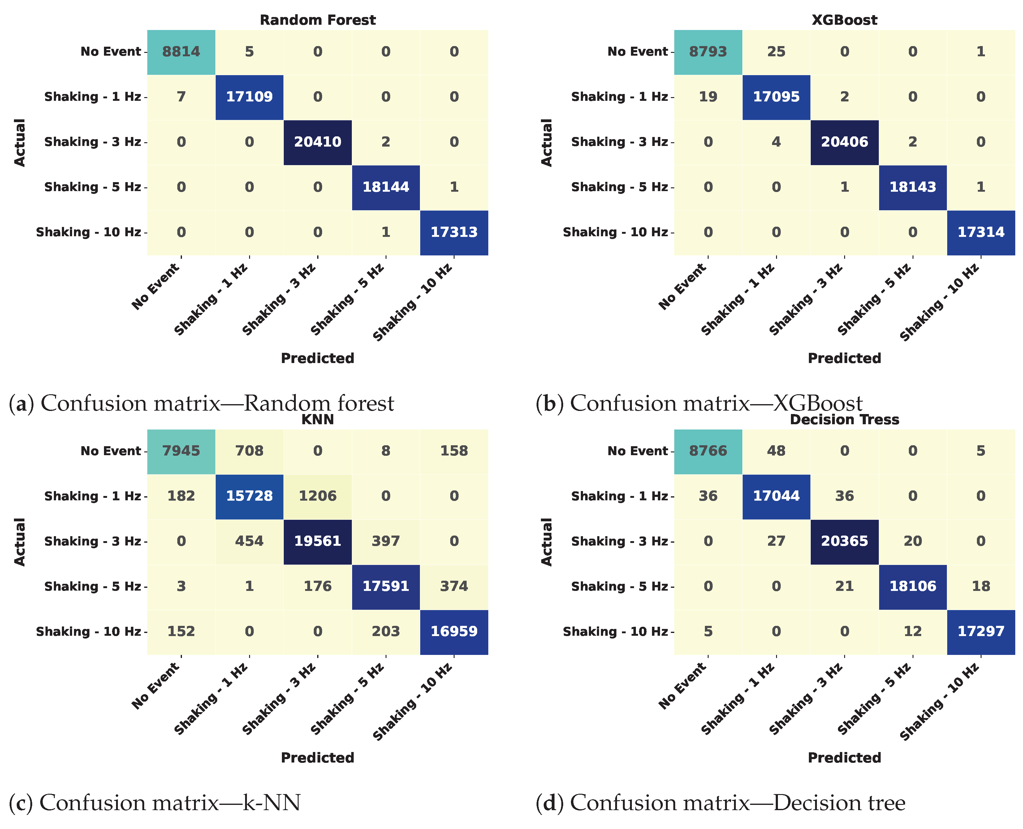
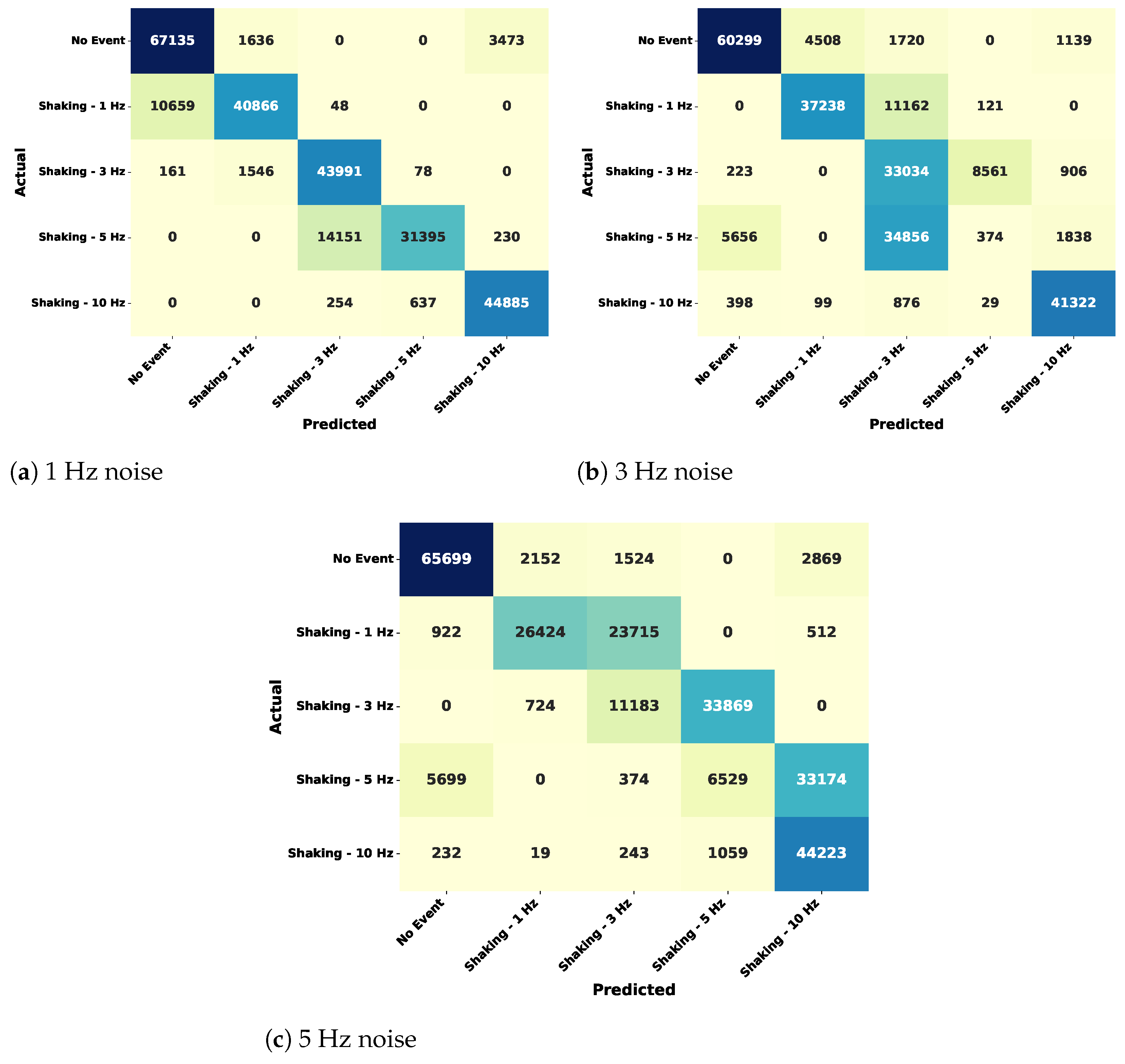
4.2.1. Confusion Matrix

The confusion matrix is a fundamental evaluation tool in supervised learning, offering a comprehensive breakdown of classification outcomes. It contrasts the actual class labels against the predicted ones to assess the model’s ability to distinguish between multiple event types. The confusion matrix shows a tabular representation consisting of actual and predicted class labels, shown in Table 3. Here, true positives (TP) and true negatives (TN) represent instances correctly classified as belonging or not belonging to a particular class, respectively. False positives (FP) correspond to instances incorrectly assigned to a class, while false negatives (FN) denote those that were wrongly excluded.
In our multi-class classification scenarios, where the classes represent discrete vibration levels including “No Event”, “Shaking—1 Hz”, “Shaking—3 Hz”, “Shaking—5 Hz”, and “Shaking—10 Hz”, the confusion matrix enables detailed per-class error analysis. By highlighting both correct predictions and misclassifications across all categories. The derived metrics from this matrix are elaborated in the subsequent sections to further quantify and compare the classification performance of different machine learning algorithms evaluated in this study.

4.2.2. Accuracy

Accuracy is a global metric that quantifies the proportion of correct predictions made by the model over the entire dataset, encompassing both correctly identified positive and negative instances across all classes. It is computed using the following formula:
Accuracy = i = 1 n T P i i = 1 n ( T P i + F P i + F N i + T N i )

4.2.3. Precision

Precision measures the exactness of the model in predicting a particular class. It is defined as the proportion of true positive predictions relative to the total number of positive predictions (both correct and incorrect) for that class:
Precision i = T P i T P i + F P i
High precision indicates a low rate of false positives, which is particularly crucial in our case, where incorrect alarms could lead to unnecessary service interruptions.

4.2.4. Recall

Recall, also known as sensitivity or true positive rate, evaluates the model’s ability to correctly identify all actual instances of a class. It is expressed as:
Recall i = T P i T P i + F N i
A high recall value implies that the model is effective in capturing all relevant instances of a class, which is vital for early detection of critical events such as high-risk vibrations within the fiber.

4.2.5. F-1 Score

The F-1 score provides a balanced assessment by harmonically combining both precision and recall for each class. It is especially useful when there is a trade-off between precision and recall, and a single metric is needed to summarize model performance:
F - 1 i = 2 × Precision i × Recall i Precision i + Recall i
The F-1 score ranges from 0 to 1, with higher values indicating better balance between precision and recall.

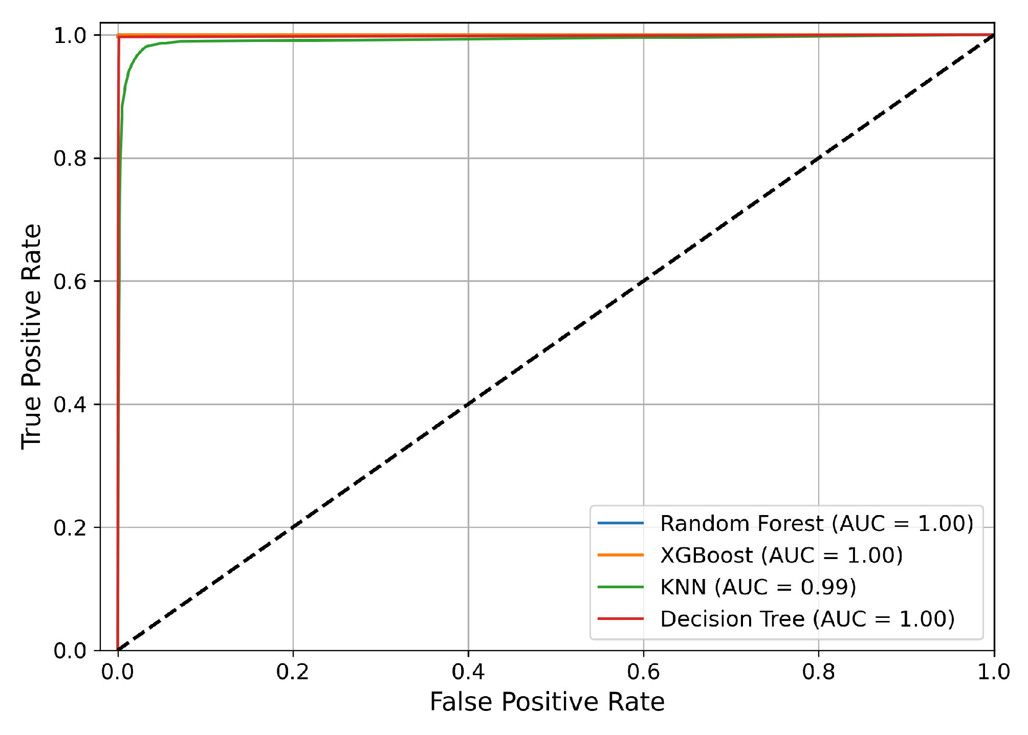
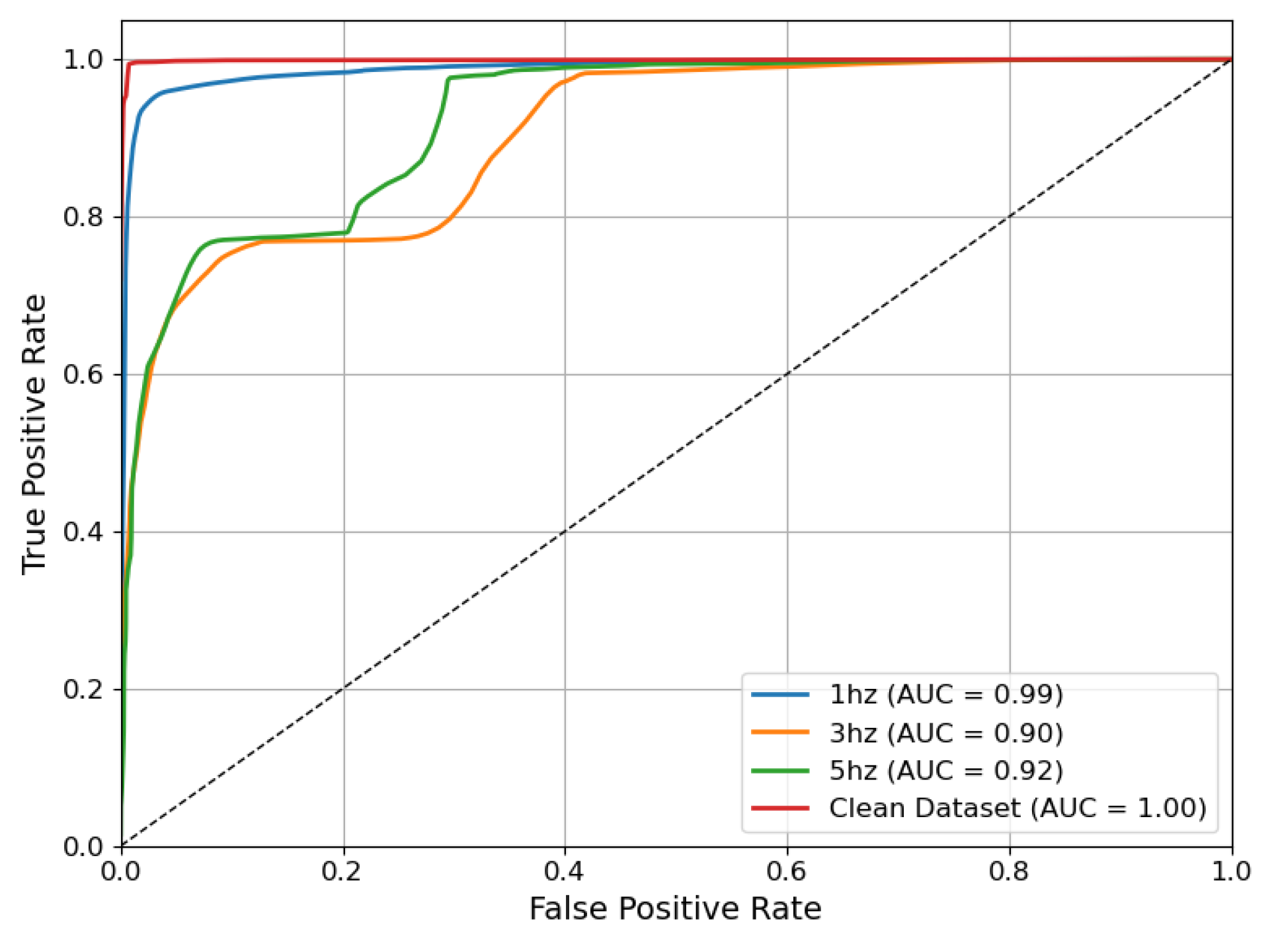
4.2.6. AUC-ROC Curve

The area under the receiver operating characteristic curve (AUC-ROC) is used to evaluate the classification performance of ML models in identifying between classes across different decision thresholds. This graph plots the true positive rate (TPR) against the false positive rate (FPR) at various classification thresholds.
In our case of multi-class classification of detection of different anomaly events, we adopt the one-vs-rest (OvR) approach, where an ROC curve is computed for each class by treating it as the positive class and the rest as the negative class. The area under each ROC curve (AUC) then shows the model’s ability to distinguish that specific class from the others.
The TPR and FPR are defined as:
TPR = T P T P + F N , FPR = F P F P + T N
The AUC value close to 1.0 indicates excellent class separability, whereas a value close to 0.5 suggests no better performance than random guessing of the model. AUC-ROC is particularly useful in our experiment as it provides insights into the model’s discriminative capability for each level of vibration event types. AUC-ROC is particularly useful in our context as it provides insight into the model’s discriminative capability for each vibration event type, independent of a fixed threshold of classification.

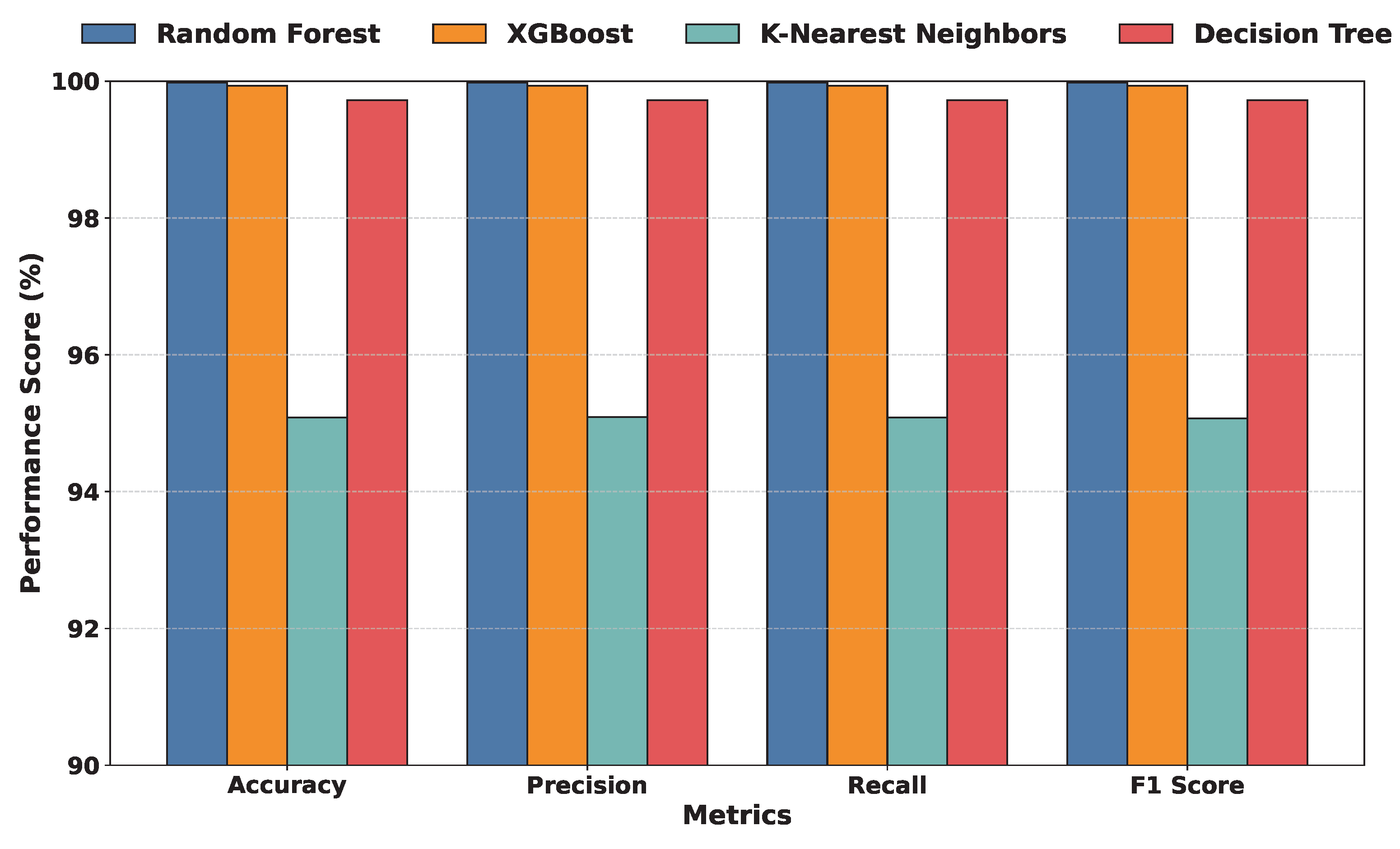
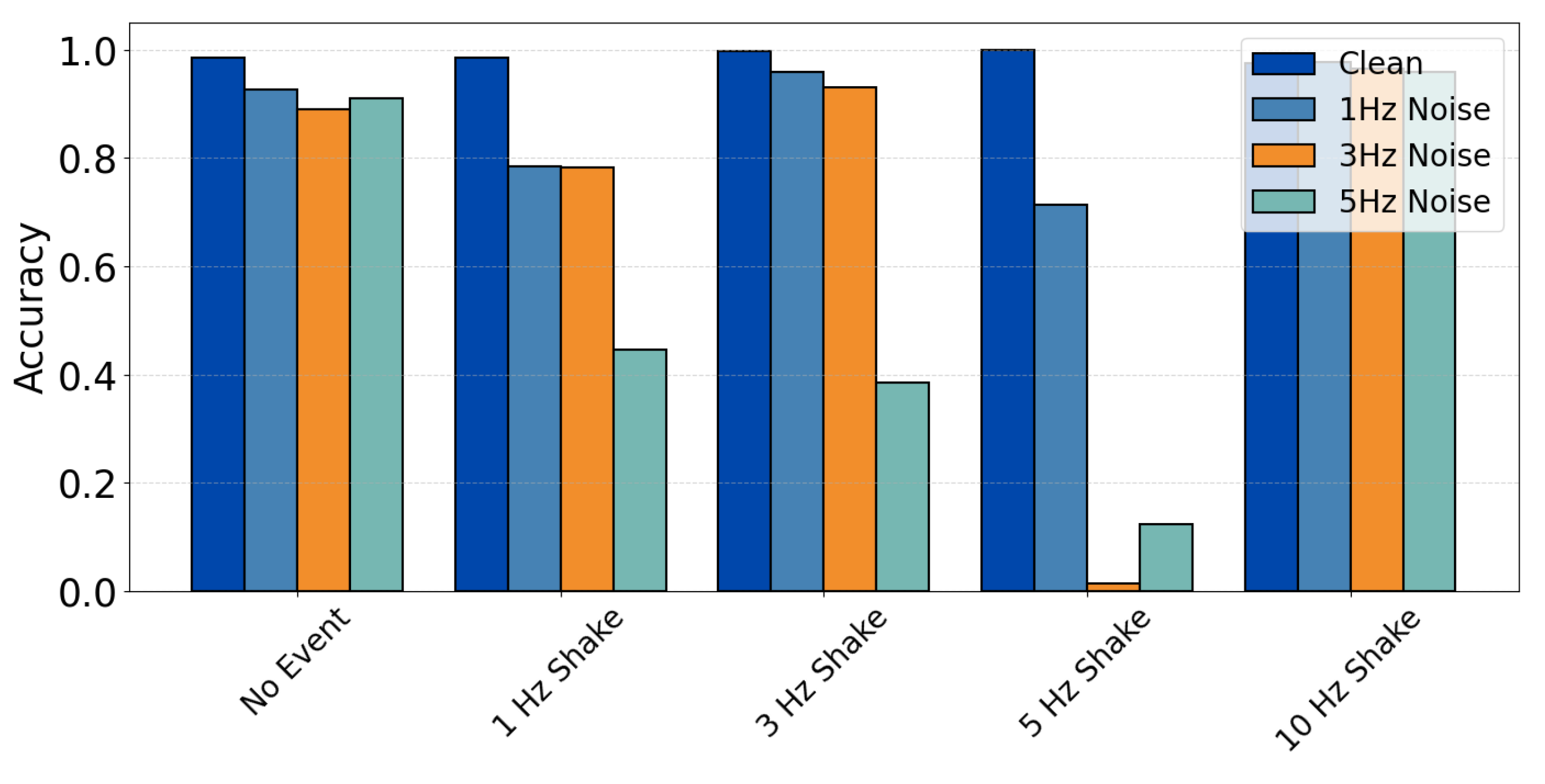
5. Performance Analysis of Machine Learning Model

This section provides a comprehensive analysis of the ML models used for vibration event classification in optical fiber networks, based on SOP dynamics. The evaluation is structured across clean and noise-augmented datasets to assess generalization and robustness.

5.1. Performance Evaluation of Model Classification Scores

Initially, all selected classifiers—random forest, XGBoost, k-NN, and decision tree—were trained and validated on a clean dataset comprising stokes parameters and SOPAS. To extract meaningful temporal patterns, we incorporated lag features (up to the third order) and rolling statistics (mean and standard deviation) as part of feature engineering.
Performance was measured using four standard metrics: Accuracy, Precision, Recall, and F-1 score, as shown in Figure 6. Random forest emerged as the most accurate classifier, achieving a near-perfect accuracy of 99.98%, followed by XGBoost and decision tree, while k-NN lagged with an accuracy of 95.08%.
Figure 7 illustrates the ROC curves of the four models trained and tested on the clean dataset. It is seen that the tree-based models, namely RF, XGBoost, and decision tree, all perform well as they all achieved an AUC score of 1.00. However, RF was better at distinguishing between the four labels in this experiment. This is because the curve for the RF is slightly higher than that for decision tree and XGBoost. This shows that the RF model is ideal for the prediction of different events compared to the other models.
Figure 8 presents the confusion matrices for all models evaluated on the clean dataset. These matrices illustrate how well each classifier predicted the five distinct event categories: No Event, and Shaking at 1 Hz, 3 Hz, 5 Hz, and 10 Hz. The RF classifier demonstrated exceptional classification performance across all categories, misclassifying only a handful of instances. It was particularly effective in differentiating between adjacent frequencies like 3 Hz and 5 Hz, which often produce overlapping SOP variations. RF constructs several decision trees using random bootstrap samples and feature subsets in this vibration classification scenario, then aggregates the results, which consequently reduces model variance and mitigates overfitting. Because of this bagging technique, RF is particularly resistant to noise and outliers in the angular speed and stokes characteristics. This highlights the model’s capability to discern subtle temporal and polarization-based patterns in the signal.
Conversely, the k-NN classifier exhibited significant misclassifications, particularly between classes with closer frequency spectra, such as 5 Hz and 10 Hz, and also struggled to separate No Event from low-frequency ambient vibrations. These misclassifications are attributed to k-NN’s reliance on local proximity in high-dimensional feature space, which is sensitive to noise and feature overlap. XGBoost and decision tree performed comparably well, though slightly below RF, with a few more errors in higher frequency shake classifications.
To quantitatively assess the impact of noise on model performance, we evaluated the RF classifier on datasets with 1 Hz, 3 Hz, and 5 Hz superimposed noise, shown in Figure 9. The resulting classification accuracies were 87.41%, 70.50%, and 58.99%, respectively. These figures reflect the expected trend of decreasing accuracy with increasing noise intensity, as noise distorts polarization fingerprints and makes class boundaries less distinguishable. However, even under severe 5 Hz noise, the model demonstrated a commendable ability to recognize patterns associated with high-risk events. These results demonstrate the model’s generalization capability and resilience to environmental distortions.
Figure 10 shows the ROC curves of the RF model tested on the clean and datasets consisting of different levels of noise. The experimental results show that the RF model had achieved a significant AUC score of 1.00. Likewise, its strong predictive capabilities are demonstrated with a high performance on the 1Hz dataset with an AUC score of 0.99, whereas the scores on the 3 Hz and 5 Hz datasets are 0.90 and 0.92, respectively. These results demonstrate that, with the introduction of various noise levels, the RF model remains robust across different sampling rates. The model demonstrated robust classification abilities across many data quality situations.
Figure 11 illustrates the confusion matrices for these noise levels, offering a more granular view of how noise affects event classification. At 1 Hz noise, the model shows minimal confusion across most classes, with high diagonal dominance indicating correct predictions. For 3 Hz noise, a slight increase in misclassifications is observed, especially between neighboring classes such as 3 Hz and 5 Hz, highlighting the growing difficulty in differentiating similar event signatures under mild interference. Under 5 Hz noise, classification errors are more prominent, particularly for lower-frequency events like No Event and 1 Hz, which are often misclassified due to overlapping polarization signatures. Nevertheless, high-risk events such as Shaking—10 Hz continue to exhibit strong predictive consistency, reflecting the model’s robustness in identifying critical anomalies even under severe environmental perturbations.
To further analyze per-class sensitivity, Figure 12 provides a side-by-side comparison of classification accuracy for each event class across clean and noisy datasets. The first bar in each group corresponds to the clean dataset with no added noise, serving as a performance baseline. As superimposed noise is introduced at increasing levels (1 Hz, 3 Hz, and 5 Hz), a progressive yet non-linear decline in classification accuracy is observed. Notably, the accuracy drops with increasing noise levels, particularly for the 1 Hz and 5 Hz shaking events. This is due to the superimposition of 3 Hz and 5 Hz noise frequency overlapping more destructively with the polarization signatures of some of the frequency events, thus creating confusion for the classifier. The sharp decline for 5 Hz shaking at this noise level further validates this, indicating that moderate-frequency noise has a disproportionately disruptive effect on the model’s prediction accuracy.
Low-frequency classes Shaking—1 Hz, 3 Hz, and 5 Hz show significant degradation as noise increases, due to their inherently subtle signal characteristics being easily masked. Meanwhile, Shaking—10 Hz maintains relatively stable accuracy, demonstrating that high-frequency events generate more distinguishable SOP patterns, which remain robust even under harsh conditions. This analysis affirms the model’s practical viability in real-world deployments where environmental interference is inevitable.
Overall, the RF model shows potential for deployment in fiber anomaly detection scenarios, delivering both high accuracy and noise robustness.

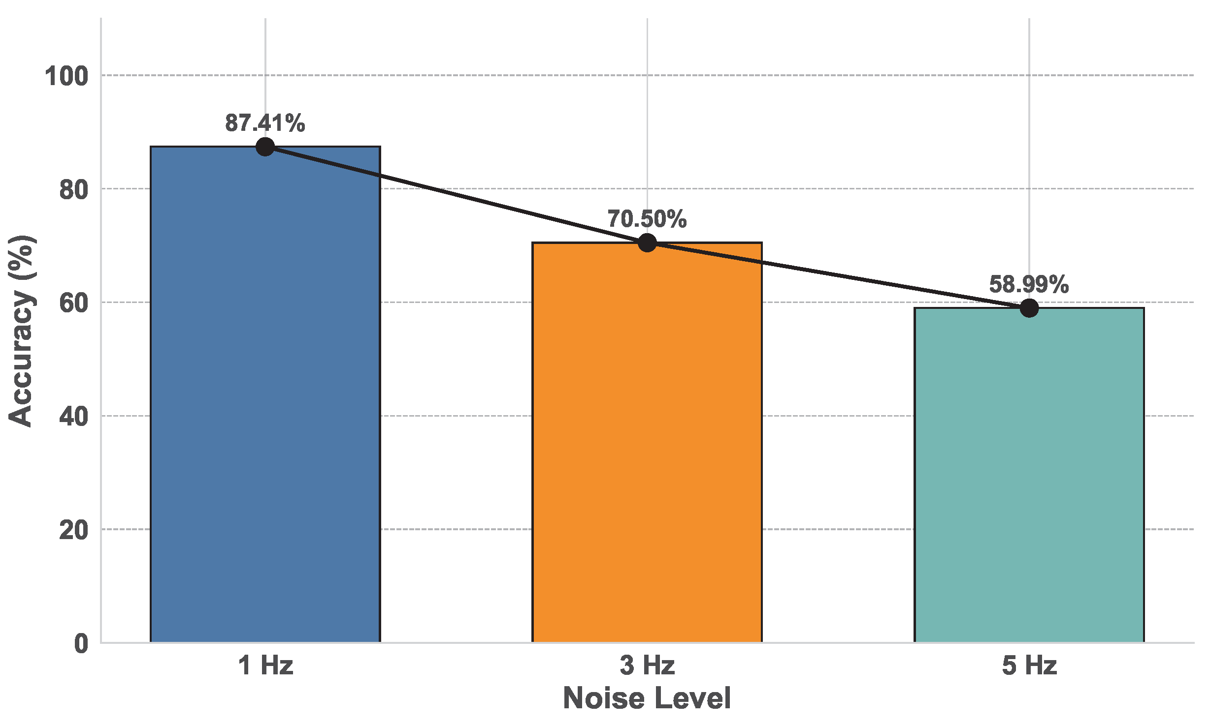
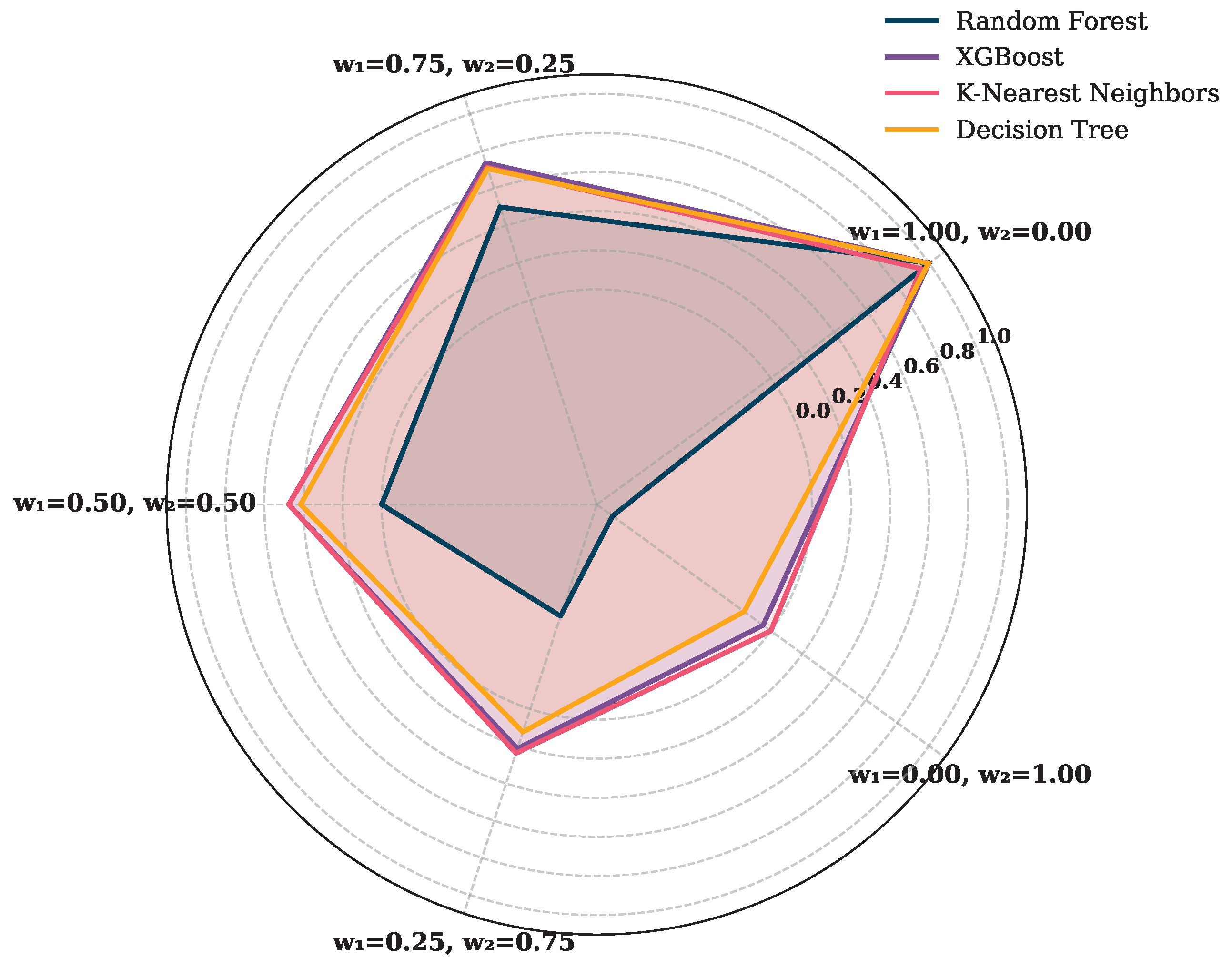
5.2. Performance Evaluation of ML Models Using Weighted Metrics

While conventional evaluation metrics, such as accuracy, precision, recall, and F-1 score, offer valuable insights into model performance, they do not account for computational efficiency, a crucial factor for real-time or resource-limited deployments. To bridge this gap, we introduced a weighted performance metric (WPM) that jointly considers classification accuracy and training time. This metric enables a comprehensive evaluation of models under varying operational priorities. The WPM for a given model i is defined as:
WPM i = w 1 · Accuracy i w 2 · TrainingTime i max ( TrainingTime i )
Here, w 1 and w 2 represent the user-defined weights for accuracy and training efficiency, respectively, and are constrained such that w 1 + w 2 = 1 . The training time of each model is normalized by the maximum training time among all models to ensure fair comparison. To explore how model performance changes under different priorities, we evaluated the WPM across five weight configurations: from complete emphasis on accuracy ( w 1 = 1.0 ,   w 2 = 0.0 ) , to equal weighting ( w 1 = 0.5 ,   w 2 = 0.5 ) , and up to full emphasis on the training efficieny ( w 1 = 0.0 ,   w 2 = 1.0 ) . The resulting WPM scores are visualized using a radar plot, defined by the Figure 13, where each axis corresponds to a specific weight combination and the radial extent denotes the WPM value for a particular classifier.
Under full emphasis on accuracy ( w 1 = 1.0 ) , the radar plot reveals that RF and XGBoost attain the highest WPM values. This reflects their strong classification performance in terms of accuracy and F-1 score. In contrast, k-NN and decision tree, while computationally efficient, are penalized due to their relatively lower predictive accuracy. As the weight gradually shifts to include training time ( w 1 = 0.75 ) , a divergence begins to appear. While XGBoost maintains a strong WPM due to its short training time, RF experiences a more noticeable reduction, given its relatively heavier computational requirements. When accuracy and training time are weighted equally ( w 1 = 0.5 ,   w 2 = 0.5 ) , the distribution of WPM scores begin to even out across models. XGBoost maintains a stable performance, while k-NN and decision tree demonstrate improved WPMs as their shorter training durations now carry greater influence. Meanwhile, RF sees a more significant decline due to the increasing penalty from its longer training time. In scenarios where computational efficiency becomes dominant ( w 1 = 0.25 ,   w 2 = 0.75 ) , the WPM values for k-NN and decision tree increase further. These models, although less accurate, are now favored due to their lightweight training profiles. Conversely, the WPM for RF continues to drop sharply, while XGBoost exhibits only a marginal decline, indicating its relatively balanced profile between accuracy and efficiency. Finally, when training time is the sole priority ( w 2 = 1.0 ) , decision tree achieves the highest WPM value, followed closely by k-NN. These models have minimal training time and are thus strongly rewarded under this weighting scheme. Both random forest and XGBoost, despite their strong classification capabilities, are significantly penalized under this configuration due to their heavy computational demands.
The radar plot clearly illustrates the trade-offs between accuracy and training time, making it a useful tool for selecting models based on specific deployment needs. By adjusting the weight given to each factor, this method allows for more practical and flexible model evaluation than relying on a single metric alone.
In the end, we have summarized the performance of four classification models (RF, XGBoost, k-NN, DT) under various noise conditions in Table 4. While all models perform well in the absence of noise, RF has the highest accuracy (99.98%) and F1-score (0.9998). The performance of RF significantly declined when the noise frequency increased from 1 to 5 Hz, according to our subsequent evaluation.

6. Conclusions

This work introduces a resilient ML framework for anomaly detection in optical networks using the SOP. The framework presented effectively identifies and classifies various threats, inlcuding eavesdropping, overlapping events, and different levels of external vibrations, by capturing and analyzing polarization fingerprints derived from polarimeter sensing. Through extensive experimentation, we demonstrated that supervised learning models, particularly random forest and XGBoost, achieve high classification accuracy (up to 99.98%) on clean datasets and exhibit strong resilience to environmental noise, maintaining reliable detection capabilities under noisy conditions. A key advantage of the proposed framework is its ability to differentiate between benign and malicious anomalies using SOP dynamics without requiring intrusive fiber instrumentation. Furthermore, the inclusion of a weighted performance metric allows for flexible model selection based on accuracy–efficiency trade-offs, making the system adaptable to different deployment scenarios.
The evaluation under realistic environmental conditions, such as mechanical disturbances or background noise, demonstrated the resilience of the framework. Despite the presence of background noise of various frequencies, the model performed reasonably well. This affirms its suitability for deployment in fiber environments where such interferences are common. Future research will focus on improving the system’s resilience to environmental interference through advanced signal processing techniques such as adaptive filtering and noise-aware feature extraction, enabling better isolation of meaningful SOP variations. Although the current framework employs computationally efficient classical machine learning models, additional optimization is required for embedded and latency-sensitive applications. Specifically, future work will explore lightweight model tuning and latency-aware feature refinement to reduce the inference time and memory footprint, facilitating seamless integration into real-time monitoring systems on resource-constrained platforms.

Author Contributions

Conceptualization, G.M., M.U.M. and M.C.M.; methodology, G.M. and M.U.M.; investigation, G.M., software, I.C.D.; resources, S.S.; visualization, G.M., I.C.D. and M.U.M.; writing—original draft preparation, G.M., I.C.D. and M.U.M.; writing—review and editing, V.C., G.M., M.U.M., I.C.D. and M.C.M.; project administration, W.W.; supervision, V.C., A.N., S.K.B., G.M.G. and J.P. All authors have read and agreed to the published version of the manuscript.

Funding

This research was funded by the project PNRR-NGEU (MUR–DM117/2023) and from the European Union’s Horizon Europe research and innovation program under grant agreement No. 101092766 (ALLEGRO Project) and MSCA-DN Nestor GA No. 101119983.

Institutional Review Board Statement

Not Applicable.

Data Availability Statement

The raw data supporting the conclusions of this article will be made available by the authors on request.

Acknowledgments

João Pedro and Antonio Napoli gratefully acknowledge support from the European Union’s Horizon RIA research and innovation program under SEASON (G.A. 101096120).

Conflicts of Interest

Author Stefano Straullu, Sai Kishore Bhyri, Gabriele Maria Galimberti, Antonio Napoli, João Pedro, Walid Wakim and Vittorio Curri declares no conflicts regarding company LINKS Foundation and Optical Networks, Nokia. The other authors declare that he has no financial or other relationships that might lead to a conflict of interest.

Abbreviations

The following abbreviations are used in this manuscript:
SOPState of Polarization
SOPASState-of-Polarization Angular Speed
MLMachine Learning
OTDROptical Time-Domain Reflectometer
DASDistributed Acoustic Sensing
DOPDegree of Polarization
OFIOptical Fiber Identification
SMFSingle Mode Fiber
LSTMLong Short-Term Memory
BiGRUBidirectional Gated Recurrent Unit
DCMData Clustering Module
SNRSignal-to-Noise Ratio
PCBPrinted Circuit Board
XGBoostExtreme Gradient Boosting
k-NNk-Nearest Neighbor
RFRandom Forest
WPMWeighted Performance Metric
TPTrue Positive
TNTrue Negative
FPFalse Positive
FNFalse Negative
AUCArea Under Curve
ROCReceiver Operating Characteristic
FPRFalse Positive Rate
OvROne-vs-Rest
TPRTrue Positive Rate
AUC-ROCArea Under the Receiver Operating Characteristic curve
CNNConvolutional Neural Network
DLDeep Learning
1D-CNNOne-Dimensional CNN

References

  1. Malik, G.; Ahmad, A.; Ahmad, A. Merging Engine Implementation with Co-Existence of Independent Dynamic Bandwidth Allocation Algorithms in Virtual Passive Optical Networks. In Proceedings of the Asia Communications and Photonics Conference 2021, Shanghai, China, 24–27 October 2021; Optica Publishing Group: Washington, DC, USA, 2021; p. T4A.273. [Google Scholar] [CrossRef]
  2. Lalou, M.; Mohammed Amin, T.; Kheddouci, H. The Critical Node Detection Problem in networks: A survey. Comput. Sci. Rev. 2018, 28, 92–117. [Google Scholar] [CrossRef]
  3. Bao, Y.; Chen, G.; Meng, W.; Tang, F.; Chen, Y. Kilometer-Long Optical Fiber Sensor for Real-Time Railroad Infrastructure Monitoring to Ensure Safe Train Operation. In Proceedings of the 2015 Joint Rail Conference, San Jose, CA, USA, 23–26 March 2015. ASME/IEEE Joint Rail Conference. [Google Scholar] [CrossRef]
  4. Edme, P.; Paitz, P.; Walter, F.; van Herwijnen, A.; Fichtner, A. Fiber-optic detection of snow avalanches using telecommunication infrastructure. arXiv 2023, arXiv:2302.12649. [Google Scholar]
  5. Awad, H.; Usmani, F.; Virgillito, E.; Bratovich, R.; Proietti, R.; Straullu, S.; Pastorelli, R.; Curri, V. A Machine Learning-Driven Smart Optical Network Grid for Earthquake Early Warning. In Proceedings of the 2024 24th International Conference on Transparent Optical Networks (ICTON), Bari, Italy, 14–18 July 2024; pp. 1–6. [Google Scholar] [CrossRef]
  6. Sifta, R.; Munster, P.; Sysel, P.; Horvath, T.; Novotny, V.; Krajsa, O.; Filka, M. Distributed fiber-optic sensor for detection and localization of acoustic vibrations. Metrol. Meas. Syst. 2015, 22, 111–118. [Google Scholar] [CrossRef]
  7. Pendão, C.; Silva, I. Optical Fiber Sensors and Sensing Networks: Overview of the Main Principles and Applications. Sensors 2022, 22, 7554. [Google Scholar] [CrossRef]
  8. Fichtner, A.; Bogris, A.; Nikas, T.; Bowden, D.; Lentas, K.; Melis, N.S.; Simos, C.; Simos, I.; Smolinski, K. Theory of phase transmission fibre-optic deformation sensing. Geophys. J. Int. 2022, 231, 1031–1039. [Google Scholar] [CrossRef]
  9. Weiqiang, Z.; Biondi, E.; Li, J.; Yin, J.; Ross, Z.; Zhan, Z. Seismic Arrival-time Picking on Distributed Acoustic Sensing Data using Semi-supervised Learning. Nat. Commun. 2023, 14, 8192. [Google Scholar] [CrossRef]
  10. Lindsey, N.; Yuan, S.; Lellouch, A.; Gualtieri, L.; Lecocq, T.; Biondi, B. City-Scale Dark Fiber DAS Measurements of Infrastructure Use During the COVID-19 Pandemic. Geophys. Res. Lett. 2020, 47, e2020GL089931. [Google Scholar] [CrossRef]
  11. Liu, J.; Yuan, S.; Dong, Y.; Biondi, B.; Noh, H. TelecomTM: A Fine-Grained and Ubiquitous Traffic Monitoring System Using Pre-Existing Telecommunication Fiber-Optic Cables as Sensors. Proc. ACM Interact. Mob. Wearable Ubiquitous Technol. 2023, 7, 64:1–64:24. [Google Scholar] [CrossRef]
  12. Natalino, C.; Schiano, M.; Di Giglio, A.; Wosinska, L.; Furdek, M. Experimental Study of Machine-Learning-Based Detection and Identification of Physical-Layer Attacks in Optical Networks. J. Light. Technol. 2019, 37, 4173–4182. [Google Scholar] [CrossRef]
  13. Mecozzi, A.; Cantono, M.; Castellanos, J.C.; Kamalov, V.; Muller, R.; Zhan, Z. Polarization sensing using submarine optical cables. Optica 2021, 8, 788–795. [Google Scholar] [CrossRef]
  14. Abdelli, K.; Cho, J.Y.; Azendorf, F.; Griesser, H.; Tropschug, C.; Pachnicke, S. Machine-learning-based anomaly detection in optical fiber monitoring. J. Opt. Commun. Netw. 2022, 14, 365–375. [Google Scholar] [CrossRef]
  15. Boitier, F.; Lemaire, V.; Pesic, J.; Chavarria, L.; Layec, P.; Bigo, S.; Dutisseuil, E. Proactive Fiber Damage Detection in Real-time Coherent Receiver. In Proceedings of the 2017 European Conference on Optical Communication (ECOC), Gothenburg, Sweden, 17–21 September 2017; pp. 1–3. [Google Scholar] [CrossRef]
  16. Abdelli, K.; Lonardi, M.; Gripp, J.; Olsson, S.; Boitier, F.; Layec, P. Breaking boundaries: Harnessing unrelated image data for robust risky event classification with scarce state of polarization data. In Proceedings of the 49th European Conference on Optical Communications (ECOC 2023), Hybrid Conference, Glasgow, UK, 1–5 October 2023; Volume 2023, pp. 924–927. [Google Scholar] [CrossRef]
  17. Abdelli, K.; Lonardi, M.; Gripp, J.; Olsson, S.; Boitier, F.; Layec, P. Computer Vision for Anomaly Detection in Optical Networks with State of Polarization Image Data: Opportunities and Challenges. In Proceedings of the 2024 24th International Conference on Transparent Optical Networks (ICTON), Bari, Italy, 14–18 July 2024; pp. 1–4. [Google Scholar] [CrossRef]
  18. Nyarko-Boateng, O.; Adekoya, A.; Weyori, B. Predicting the Actual Location of Faults in Underground Optical Networks using Linear Regression. Eng. Rep. 2020, 3, eng212304. [Google Scholar] [CrossRef]
  19. Lecun, Y.; Bottou, L.; Bengio, Y.; Haffner, P. Gradient-based learning applied to document recognition. Proc. IEEE 1998, 86, 2278–2324. [Google Scholar] [CrossRef]
  20. Abdelli, K.; Grießer, H.; Ehrle, P.; Tropschug, C.; Pachnicke, S. Reflective fiber fault detection and characterization using long short-term memory. J. Opt. Commun. Netw. 2021, 13, E32–E41. [Google Scholar] [CrossRef]
  21. Zhang, W.; Li, C.; Peng, G.; Chen, Y.; Zhang, Z. A deep convolutional neural network with new training methods for bearing fault diagnosis under noisy environment and different working load. Mech. Syst. Signal Process. 2018, 100, 439–453. [Google Scholar] [CrossRef]
  22. Sadighi, L.; Karlsson, S.; Natalino, C.; Wosinska, L.; Ruffini, M.; Furdek, M. Deep Learning for Detection of Harmful Events in Real-World, Noisy Optical Fiber Deployments. J. Light. Technol. 2025, 1–9. [Google Scholar] [CrossRef]
  23. Chen, X.; Li, B.; Proietti, R.; Zhu, Z.; Yoo, S.J.B. Self-Taught Anomaly Detection With Hybrid Unsupervised/Supervised Machine Learning in Optical Networks. J. Light. Technol. 2019, 37, 1742–1749. [Google Scholar] [CrossRef]
  24. Tomasov, A.; Dejdar, P.; Munster, P.; Horvath, T.; Barcik, P.; Da Ros, F. Enhancing fiber security using a simple state of polarization analyzer and machine learning. Opt. Laser Technol. 2023, 167, 109668. [Google Scholar] [CrossRef]
  25. Sadighi, L.; Karlsson, S.; Natalino, C.; Furdek, M. Machine Learning-Based Polarization Signature Analysis for Detection and Categorization of Eavesdropping and Harmful Events. In Proceedings of the 2024 Optical Fiber Communications Conference and Exhibition (OFC), San Diego, CA, USA, 24–28 March 2024; pp. 1–3. [Google Scholar]
  26. Sadighi, L.; Karlsson, S.; Natalino, C.; Wosinska, L.; Ruffini, M.; Furdek, M. Detection and Classification of Eavesdropping and Mechanical Vibrations in Fiber Optical Networks by Analyzing Polarization Signatures Over a Noisy Environment. In Proceedings of the ECOC 2024; 50th European Conference on Optical Communication, Frankfurt, German, 22–26 September 2024; pp. 527–530. [Google Scholar]
  27. Sadighi, L.; Karlsson, S.; Wosinska, L.; Furdek, M. Machine Learning Analysis of Polarization Signatures for Distinguishing Harmful from Non-harmful Fiber Events. In Proceedings of the 2024 24th International Conference on Transparent Optical Networks (ICTON), Bari, Italy, 14–18 July 2024; pp. 1–5. [Google Scholar] [CrossRef]
  28. Malik, G.; Masood, M.U.; Dipto, I.C.; Mohamed, M.C.; Straullu, S.; Bhyri, S.K.; Galembirti, G.M.; Pedro, J.; Napoli, A.; Wakim, W.; et al. SOP-Based Anomaly Detection Leveraging Machine Learning for Proactive Optical Restoration. In Proceedings of the Optical Network Design and Modelling ONDM, Pisa, Italy, 6–9 May 2025. [Google Scholar]
  29. Malik, G.; Masood, M.U.; Mohamed, M.C.; Straullu, S.; Bhyri, S.K.; Galembirti, G.M.; Pedro, J.; Napoli, A.; Wakim, W.; Curri, V. Machine Learning for Predictive Multi-Event Detection in Fiber Optic Systems. In Proceedings of the IEEE International Conference on Machine Learning for Communication and Networking (ICMLCN), Barcelona, Spain, 26–29 May 2025. [Google Scholar]
  30. Malik, G.; Masood, M.U.; Dipto, I.C.; Mohamed, M.C.; Straullu, S.; Bhyri, S.K.; Galembirti, G.M.; Pedro, J.; Napoli, A.; Wakim, W.; et al. Intelligent Detection of Overlapping Fiber Anomalies in Optical Networks Using Machine Learning. In Proceedings of the IEEE Summer Topicals, Berlin, Germany, 21–23 July 2025. [Google Scholar]
  31. Zhang, X.; Gu, C.; Lin, J. Support vector machines for anomaly detection. In Proceedings of the 2006 6th World Congress on Intelligent Control and Automation, Dalian, China, 21–23 June 2006; Volume 1, pp. 2594–2598. [Google Scholar]
  32. Abdelli, K.; Lonardi, M.; Gripp, J.; Correa, D.; Olsson, S.; Boitier, F.; Layec, P. Anomaly detection and localization in optical networks using vision transformer and SOP monitoring. In Optical Fiber Communication Conference; Optica Publishing Group: Washington, DC, USA, 2024; p. Tu2J.4. [Google Scholar]
  33. Collett, E. Field Guide to Polarization; SPIE Digital Library; SPIE: Bellingham, WA, USA, 2005. [Google Scholar] [CrossRef]
  34. Pellegrini, S.; Rizzelli, G.; Barla, M.; Gaudino, R. Algorithm optimization for rockfalls alarm system based on fiber polarization sensing. IEEE Photonics J. 2023, 15, 7100709. [Google Scholar] [CrossRef]
  35. Tosi, D.; Sypabekova, M.; Bekmurzayeva, A.; Molardi, C.; Dukenbayev, K. 2—Principles of fiber optic sensors. In Optical Fiber Biosensors; Tosi, D., Sypabekova, M., Bekmurzayeva, A., Molardi, C., Dukenbayev, K., Eds.; Academic Press: Cambridge, MA, USA, 2022; pp. 19–78. [Google Scholar] [CrossRef]
  36. Zafar Iqbal, M.; Fathallah, H.; Belhadj, N. Optical fiber tapping: Methods and precautions. In Proceedings of the 8th International Conference on High-Capacity Optical Networks and Emerging Technologies, Riyadh, Saudi Arabia, 19–21 December 2011; pp. 164–168. [Google Scholar] [CrossRef]
  37. Song, H.; Lin, R.; Li, Y.; Lei, Q.; Zhao, Y.; Wosinska, L.; Monti, P.; Zhang, J. Machine-learning-based method for fiber-bending eavesdropping detection. Opt. Lett. 2023, 48, 3183–3186. [Google Scholar] [CrossRef]
  38. Yilmaz, A.K.; Deniz, A.; Yuksel, H. Experimental Optical Setup to Measure Power Loss versus Fiber Bent Radius for Tapping into Optical Fiber Communication Links. In Proceedings of the 2021 International Conference on Electrical, Computer and Energy Technologies (ICECET), Cape Town, South Africa, 9–10 December 2021; pp. 1–6. [Google Scholar] [CrossRef]
  39. Lei, Q.; Li, Y.; Song, H.; Wang, W.; Zhao, Y.; Zhang, J.; Liu, Y. Multi-intensity Bending Eavesdropping Detection and Identification Scheme Based on the State of Polarization. In Proceedings of the 2023 Opto-Electronics and Communications Conference (OECC), Shanghai, China, 2–6 July 2023; pp. 1–4. [Google Scholar] [CrossRef]
  40. Spurny, V.; Dejdar, P.; Tomasov, A.; Munster, P.; Horvath, T. Eavesdropping Vulnerabilities in Optical Fiber Networks: Investigating Macro-Bending-Based Attacks Using Clip-on Couplers. In Proceedings of the 2023 International Workshop on Fiber Optics on Access Networks (FOAN), Gent, Belgium, 30–31 October 2023; pp. 47–51. [Google Scholar] [CrossRef]
  41. Zhang, C.; Wang, D.; Wang, L.; Guan, L.; Yang, H.; Zhang, Z.; Chen, X.; Zhang, M. Cause-aware failure detection using an interpretable XGBoost for optical networks. Opt. Express 2021, 29, 31974–31992. [Google Scholar] [CrossRef] [PubMed]
  42. Cruzes, S. Failure Management Overview in Optical Networks. IEEE Access 2024, 12, 169170–169193. [Google Scholar] [CrossRef]
  43. Zhang, Z. Introduction to machine learning: K-nearest neighbors. Ann. Transl. Med. 2016, 4, 218. [Google Scholar] [CrossRef] [PubMed]
  44. Quinlan, J.R. Learning decision tree classifiers. ACM Comput. Surv. (CSUR) 1996, 28, 71–72. [Google Scholar] [CrossRef]
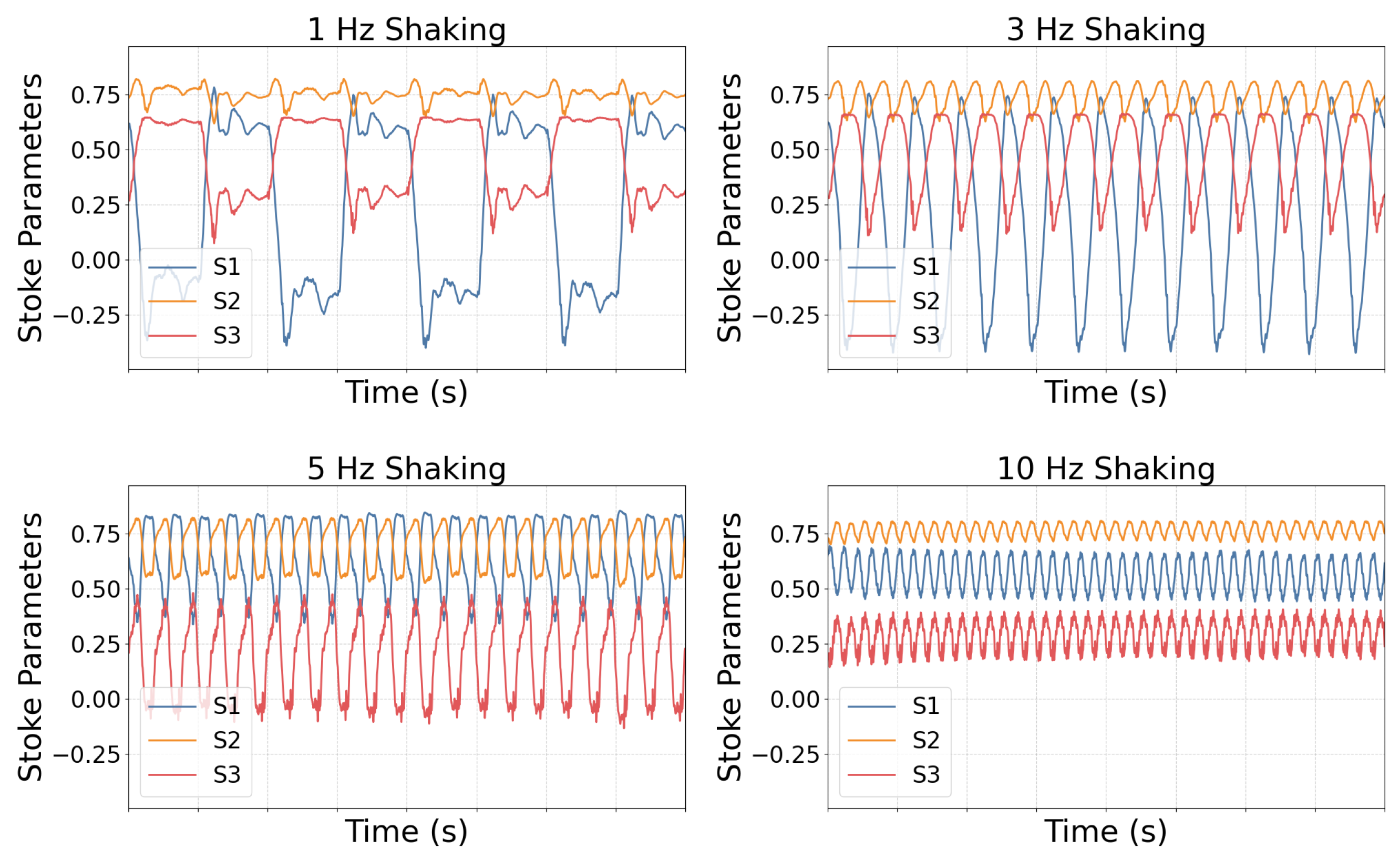
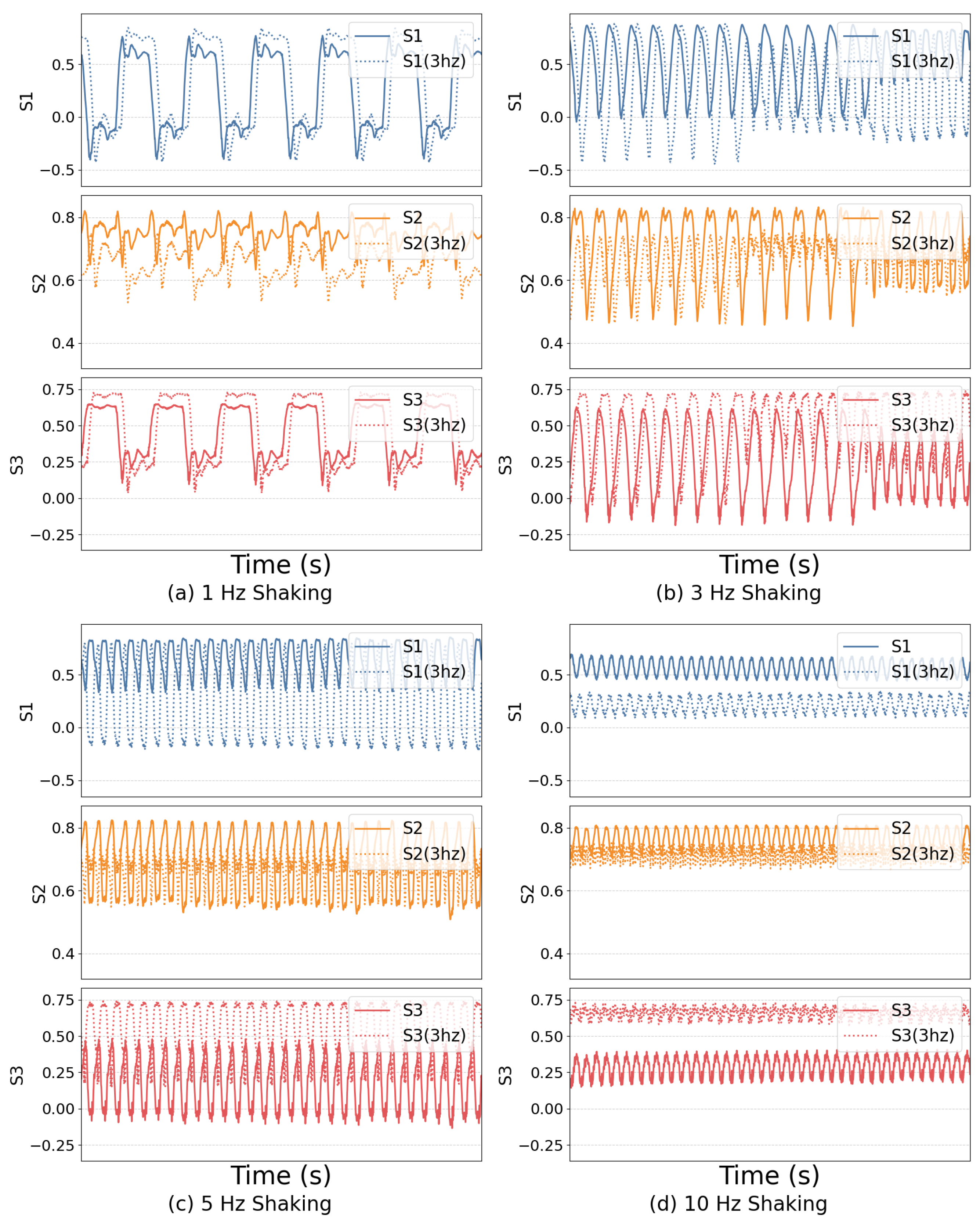
Figure 1. Bending for various experiments using OFI.
Ai 06 00131 g001
Figure 2. Simultaneous occurrence of bending and tapping.
Ai 06 00131 g002
Figure 3. Stoke parameters plot for the clean dataset.
Ai 06 00131 g003
Figure 4. Stokes parameter variations under 3 Hz noise perturbation.
Ai 06 00131 g004
Figure 5. Flowchart of the machine learning framework for predictive modeling.
Ai 06 00131 g005
Figure 6. Comparison of metrics of the models trained on the clean dataset.
Ai 06 00131 g006
Figure 7. AUC-ROC curves of the different models on clean dataset.
Ai 06 00131 g007
Figure 8. Confusion metrics of all the models after testing on the clean data.
Ai 06 00131 g008
Figure 9. Accuracy scores of the random forest model tested on the datasets with various noise levels.
Ai 06 00131 g009
Figure 10. AUC-ROC curves of the random forest model on clean and noisy datasets.
Ai 06 00131 g010
Figure 11. Confusion matrix for testing on different noise levels.
Ai 06 00131 g011
Figure 12. Comparison of per-event accuracy of clean data with different noise levels.
Ai 06 00131 g012
Figure 13. Radar plot of WPM scores illustrating accuracy–efficiency trade-offs.
Ai 06 00131 g013
Table 1. Categorization of vibration events.
Event TypeSeverity LevelDescription
No eventNoneNormal operations with no impact on fiber integrity
Shaking (1 Hz)LowAmbient noise due to environmental activities
Shaking (3 Hz)ModerateMinor disturbances caused by nearby environment
Shaking (5 Hz)HighSustained mechanical stress
Shaking (10 Hz)CriticalCritical intrusion
Table 2. Features used for training the ML models.
Feature TypeVariable TypeFeature Examples
Input Features m 1 S 1 , S 2 , S 3 , w [ k ]
Rolling Mean (Win = 500, 1000) m 2 , m 3 rolling _ mean _ S 1 _ 3 , , rolling _ mean _ w [ k ] _ 5
Rolling Std Dev (Win = 500, 1000) m 4 , m 5 rolling _ std _ S 1 _ 3 , , rolling _ std _ w [ k ] _ 5
Lag Features (Lag = 1, 2, 3) m 6 , m 7 , m 8 lag _ S 1 _ 1 , , lag _ w [ k ] _ 3
Table 3. Structure of confusion matrix.
Predicted PositivePredicted Negative
Actual PositiveTPFN
Actual NegativeFPTN
Table 4. Performance evaluation of classification models under different noise frequencies.
Accuracy (%)F-1 Score
ScenarioRFXGBoostk-NNDTRFXGBoostk-NNDT
No noise99.9899.9395.0899.720.99980.99930.95070.9972
1 Hz noise87.5---0.873---
3 Hz noise70.50---0.699---
5 Hz noise58.99---0.578---
Disclaimer/Publisher’s Note: The statements, opinions and data contained in all publications are solely those of the individual author(s) and contributor(s) and not of MDPI and/or the editor(s). MDPI and/or the editor(s) disclaim responsibility for any injury to people or property resulting from any ideas, methods, instructions or products referred to in the content.

