Abnormal Alliance Detection Method Based on a Dynamic Community Identification and Tracking Method for Time-Varying Bipartite Networks

Abstract

Identifying abnormal group behavior formed by multi-type participants from large-scale historical industry and tax data is important for regulators to prevent potential criminal activity. We propose an Abnormal Alliance detection framework comprising two methods. For detecting joint behavior among multi-type participants, we present DyCIAComDet, a dynamic community identification and tracking method for large-scale, time-varying bipartite multi-type participant networks, and introduce three community-splitting measurement indicators—cohesion, integration, and leadership—to improve community division. To verify whether joint behavior is abnormal, termed an Abnormal Alliance, we propose BMPS, a frequent-sequence identification algorithm that mines key features along community evolution paths based on bitmap matrices, sequence matrices, prefix-projection matrices, and repeated-projection matrices. The framework is designed to address sampling limitations, temporal issues, and subjectivity that hinder traditional analyses and to remain scalable to large datasets. Experiments on the Southern Women benchmark and a real tax dataset show DyCIAComDet yields a mean modularity Q improvement of 24.6% over traditional community detection algorithms. Compared with PrefixSpan, BMPS improves mean time and space efficiency by up to 34.8% and 35.3%, respectively. Together, DyCIAComDet and BMPS constitute an effective, scalable detection pipeline for identifying abnormal alliances in tax datasets and supporting regulatory analysis.

1. Introduction

In the field of tax administration, abnormal group behavior such as false invoicing, income concealment, tax evasion, and tax fraud are prevalent and significantly impact the healthy operation of tax collection and the economic ecosystem [1]. Based on large-scale historical tax data, efficiently and effectively identifying abnormal group behavior from tax-related data, including taxpayers and tax officials, is an urgent need for tax regulatory departments and a key focus of this paper’s research [2].

As far as group behavior analysis is concerned, a variety of group behavior systems can be transformed into complex networks, such as economic systems [1], biological systems [3], community ecosystems [4], and other complex systems [5]. Theoretically, many complex systems can be described by using complex networks and graphs [6]. Most real-world networks possess community structures, meaning that a large network can be divided into several sub-communities, which are tightly connected internally but sparsely connected externally [7]. Community detection algorithms are of great significance for understanding network topology, mining implicit patterns, and predicting network behavior, and are applied in multiple fields.

Especially for bipartite networks, an important and extraordinary type of complex network, it is a structural manifestation of group behavior in complex networks. Its main characteristics are as follows: (1) it consists of two different types of nodes; (2) nodes are typically divided into two disjoint sets; (3) nodes within each set are of the same type, while nodes from different sets are of different types; (4) connections only exist between the two types of nodes; that is, there are no connections between nodes within the same node type, but there are connections between nodes from different nodes types.

As the bipartite network shown in Figure 1, ellipses represent node type 1, called U-type, and rectangles represent node type 2, called V-type, with edges existing between nodes of different types and no edges between nodes of the same type. In special cases, there may be instances where nodes of the same type are connected by edges, but these are generally disregarded, and the network is still considered a bipartite network.

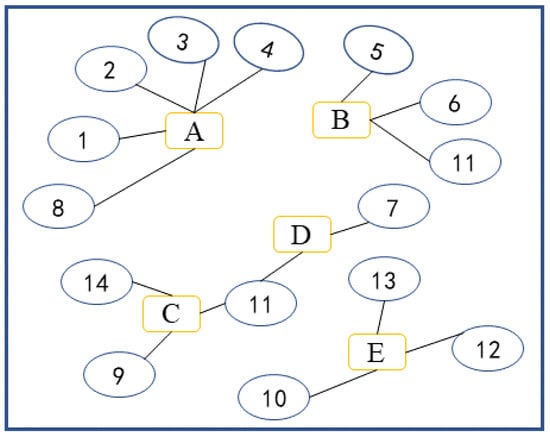
Figure 1. Illustration of a bipartite network.

Many networks in nature exhibit bipartite structures, such as taxpayer–tax officer networks [2], author–paper networks [8,9], investor–shareholder networks [10,11], viewer–movie networks [12], customer–product networks [13], and disease–gene networks [14]. In the face of the huge amount of data generated by illegal activities, such as issuing false value-added tax invoices in the process of tax supervision, it is essential to effectively overcome the problem of traditional methods being unable to analyze the temporal evolution characteristics of illegal activities based on identifying the characteristics of illegal activities.

Thus, we propose an anomaly detection method to mine temporal evolution characteristics of multi-type participants’ illegal activities, including two progressive processes. Multi-type-participant joint behavior is detected by means of the tax multi-type-participant anomaly detection module, which specifically introduces the DyCIAComDet (Dynamic CIA Community Detection Method) algorithm proposed. Then the other module is the key feature identification module for tax anomalies, which proposes the BMPS (Bitmap-based PrefixSpan algorithm) frequent sequence-mining algorithm.

In DyCIAComDet, this paper proposes an algorithm for the evolution recognition of community structures in time-varying bipartite networks. The method includes three core steps: first, we introduce the CIA algorithm for identifying community structures in static bipartite networks; second, we propose indicators that include cohesion and integration for discovering the “leadership” metric to measure the closeness between communities at adjacent timestamps; then, to verify whether the cooperative behavior has the characteristics of illegal behavior, we propose a recursive formula to incorporate cohesion and integration indicators into the calculation of the modularity Q value of community partitions over time. Furthermore, considering the time characteristic of large-scale tax data, the taxpayer–tax officer network is actually a time-varying bipartite network. This paper proposes a dynamic bipartite network community evolution algorithm based on the static CIA algorithm, namely the DyCIAComDet algorithm. The algorithm slices the dataset by timestamps. At the initial time epoch $T_0$, the corresponding bipartite network, denoted as Network $T_0$, uses the static CIA algorithm to confirm the community structure and denote the leadership nodes within these communities. For the new node data from time epoch $T_0$ to $T_1$, it quantifies the connection relationship with the leadership nodes of the historical communities at time epoch $T_0$ (i.e., historical features). If the historical features are satisfied, these nodes are ascribed to the historical communities. For the node data at time epoch $T_1$ that do not belong to any historical communities, the static CIA algorithm is applied for community detection, and the leadership nodes of the detected communities are calculated for the next iteration. The above processes are iterated by timestamps until the final time epoch Tf or all data nodes possessing community labels, at which the algorithm stops.

Finally, based on the statistical characteristics of the communities discovered by the DyCIAComDet algorithm, two types of communities are ascribed, namely ComType1-“scalper” and ComType2-“Abnormal Alliance”, which correspond to two types of actual abnormal group behavior. Key feature extraction is performed on ComType2, corresponding to the verification of abnormal group features. BMPS (bitmap frequent sequence-mining method), based on bitmap, sequence matrix, and projection matrix, is proposed, which can overcome the huge repeated scanning of the database; thus, the efficiency is greatly improved. The evolutionary path of ComType2 in the time-varying bipartite network is extracted, along with key features of their temporal paths, namely the frequently appearing node sequences. Finally, this paper innovatively proposes the BMPS algorithm (a frequent sequence-mining algorithm based on bitmap and PrefixSpan algorithm to avoid repeated scanning of the projection matrix), which is based on PrefixSpan, bitmap matrices, and the theorem of repeated projection matrices. BMPS addresses the bottleneck issue of high-frequency repetitive scanning of the database in large-scale datasets, thereby greatly improving the spatiotemporal efficiency of frequent sequence identification on large-scale sequence sets.

2. Literature Review

2.1. Community Evolutionary Algorithms for Bipartite Network

Bipartite networks are ubiquitous in nature and society, such as scientist–paper collaboration networks, person–location networks, actor–movie collaboration networks, and so on. There are typically two approaches to community detection in bipartite networks: the mapping approach and the direct approach.

The mapping method involves transforming a bipartite network into a unipartite network based on the shared nodes between the two types of nodes, and then employing established community detection algorithms designed for unipartite networks to identify community structures. The principle behind the mapping method is relatively straightforward, but it leads to a loss of network structural information, which can potentially cause significant errors in the detection of the entire community structure. Guimera et al. [15] have demonstrated that using the mapping method for community detection can yield erroneous results and even affect the community structure of the entire network. Barber [16] presented different outcomes for community detection in real bipartite networks and their corresponding projected unipartite networks, thereby confirming that the mapping method for bipartite networks is not advisable.

Guimera et al. [15] proposed a new community detection algorithm for bipartite networks based on bipartite modularity extended from unipartite modularity. Barber et al. [16] extended Newman’s modularity from unipartite networks to bipartite networks and introduced the adaptive BRIM algorithm for community detection, which is, however, limited to small-scale bipartite networks. Murata [17] also proposed a bipartite network community detection method based on bipartite modularity and demonstrated that its performance is comparable to that of unipartite network modularity. Furthermore, Liu et al. [18] presented a community detection and analysis algorithm based on label propagation for large-scale bipartite networks.

Recently, Raghavan et al. [19] proposed the Label Propagation Algorithm (LPA), a widely used method for community detection in bipartite networks. Subsequently, Li et al. [20] proposed a novel quantitative community detection method based on bipartite partition density in bipartite networks, which is better than Barber’s bipartite modularity and others. Chang et al. [21] introduced an overlapping community detection approach based on Bi-EgoNet in bipartite networks, and Wang Yang et al. [22] proposed a method for bipartite network community detection based on comparative definitions and community force.

Although community detection methods are crucial for uncovering complex network structures, the heterogeneous nature of nodes in bipartite networks presents significant challenges in accurately clustering networks with community centrality features. Furthermore, existing approaches often fail to fully capture the dynamic structural evolution that occurs during the evolution of bipartite networks.

2.2. Sequence Pattern Mining

Sequence pattern mining holds significant practical value in various application domains, such as personalized recommendations and customer behavior analysis. For instance, it can be used to deliver personalized web page recommendations based on the sequence in which users visit websites, or to optimize product promotion strategies based on patterns in customers’ daily shopping habits.

Classic sequence pattern mining algorithms are usually divided into two main categories: the first category is based on the candidate generation–test idea, utilizing the Apriori property, such as the AprioriAll [23] algorithm and the AprioriSome [23] algorithm. The logic of these two algorithms is equivalent to a breadth-first search strategy on the concept lattice constructed by the data items of the sequence database. One downside of the first category is the large scale of candidate sequences and multiple scans of the database, which leads to low efficiency in both time and space, thus reducing its feasibility in big data scenarios.

R. Agrawal proposed a constraint-based sequence pattern mining algorithm based on the Apriori property, known as the GSP algorithm [24] (Generalized Sequential Pattern), which can effectively discover frequent patterns in small-scale sequence datasets. However, when dealing with large-scale datasets, the efficiency of the algorithm significantly decreases. Additionally, in scenarios involving long sequence data, a large number of candidate sequences is generated, leading to a substantial increase in time and space.

To address these issues, Ayres et al. proposed the SPAM algorithm [25], which employs a vertical bitmap representation and bitwise operations (e.g., AND and bit-count) to compute supports of candidate sequences efficiently; however, SPAM’s bitmap structures can become memory-intensive for large-scale or long-sequence datasets.

The second category of algorithms is based on ideas of divide-and-conquer and pattern growth, such as FP-Growth [26], FreeSpan [27], and PrefixSpan [28]. Among these, PrefixSpan is a prefix-projection sequence-growth algorithm: for each frequent prefix, it recursively projects the database and grows patterns within the projected database, avoiding exhaustive candidate generation and repeated full-database scans.

In summary, these growth-based methods significantly reduce candidate generation and database scans, improving scalability. Nevertheless, bitmap-based approaches (such as SPAM) trade reduced I/O for increased memory footprint; practical approaches must balance preprocessing/memory costs and subsequent mining efficiency depending on data scale and sequence length.

3. Abnormal Alliance Detection Framework

Our Abnormal Alliance detection framework includes three parts: first, the static CIA algorithm framework proposed is designed to better detect communities in a bipartite network that possesses network centrality of networks; then, we propose a Dynamic Community Structure Discovery Algorithm on Bipartite Networks based on the CIA algorithm framework to detect the evolution of community structures in large-scale time-varying bipartite networks; finally, a frequent sequence identification algorithm (BMPS algorithm) is proposed to identify tax-related anomalous behavior.

3.1. Static CIA Algorithm Framework

Based on community cohesion and integration force, this paper proposes a static bipartite network community detection method called CIA. The framework of this algorithm is shown in Figure 2.

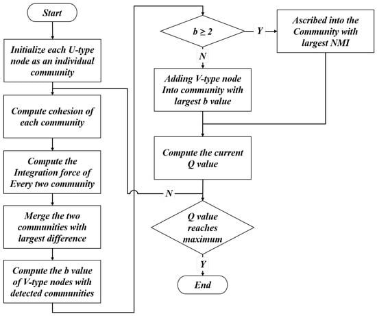
Figure 2. Flowchart of the Static CIA Algorithm.

Step 1: Denote the nodes of the bipartite network as U-type and V-type. At time epoch $T_0$, each U-type node is treated as one individual community, and they are denoted as $C_1$, $C_2$, …,$C_g$, where g is the total number of U-type nodes. In a bipartite network $G=(U,V,E)$, U represents the node set of the first type, V represents the node set of the second type, and E represents the edge set connecting nodes of these two types. For any node $u_i$ in U, the list of all nodes in V that are connected to $u_i$ is called the neighborhood list of node $u_i$. This is defined by Formula (1).

$$N\left(u_i\right)=\left\{v_j{w}_{ij}\mid v_j\in V,(u_i,v_j)\in E\right\}$$

(1)

where $w_{ij}$ is the edge weight connecting node $u_i$ and node $v_j$. It indicates that there may exist duplicate nodes within the neighbor node list of $u_i$, and weight $w_{ij}$ also reflects the connection closeness between $u_i^{\prime }s$ neighboring nodes and $u_i$. In other words, the higher the weight, the closer the connection.

Step 2: Calculate each community cohesion according to Formula (2) for discovering key nodes in the community or network. Community cohesion is a pattern that is similar to the concept of centrality of networks; nodes with the maximum degree within a network or community are usually regarded as the core nodes of that network or community. Moreover, nodes with higher degrees are connected with high probability; thus, they bear a higher probability of belonging to the same community.

$$C\left(C^U\right)=\left|N\left(C^U\right)\right|/\left(\sum _{i=0}^{|C^U|}\sum _{v_j\in N\left(u_i\right)}{w}_{ij}\right),u_i\in C^U$$

(2)

$D\left(u_i\right)$ represents the degree of node $u_i$; $C^U$ denotes a community consisting solely of U-type nodes. $|C^U|$ denotes the number of nodes in community $C^U$; $\left|N\right(C^U\left)\right|$ represents the count of common neighbors among all U-type nodes in community $C^U$. The denominator part represents the sum of edge weights of all U-type nodes in community $C^U$.

Step 3: The community integration force reflects a measurable criterion for determining whether two small communities can merge into a larger one. The greater the number of common neighbors shared between two communities, the higher the similarity between them. According to the community integration force Formula (3), calculate the integration force between every pair of communities obtained in Step 1.

$$IN({C_i}^U,{C_j}^U)={\displaystyle \frac{{\sum }_{v_j\in N({C_i}^U,{C_j}^U)}{\sum }_{u_i\in {C_i}^U\cup {C_j}^U}{w}_{u_i{v}_j}}{|{C_i}^U|+|{C_j}^U|}}$$

(3)

$N(C_i^U,C_j^U)$ denotes the set of common neighbors between communities $C_i^U$ and $C_j^U$, while $|C_i^U|$ and $|C_j^U|$ represent the number of nodes in $C_i^U$ and $C_j^U$, respectively.

Step 4: Calculate the $I{N}_{\mathrm{Minus}}(C_i,C_j)=1.87·IN(C_i^U,C_j^U)-C\left(C_i^U\right)-C\left(C_j^U\right)$, merge communities with the greatest difference.

Step 5: For each $v_i\in V$, merge $v_j$ into community $C_b$ according to $b=argmax\left({\displaystyle \frac{|N\left(v_j\right)\bigcap C_k|}{|C_k|}}\right)$. If $b\ge 2$, then merge $v_j$ into the community corresponding to the largest NMI calculated according to Formula (4).

$$NM{I}_{CD}={\displaystyle \frac{-2{\sum }_{i=1}^{N^C}{\sum }_{j=1}^{N^D}{n}_{ij}^{CD}{log}_{10}\left(\frac{n_{ij}^{CD}M}{n_i^C{n}_j^D}\right)}{{\sum }_{i=1}^{N^C}{n}_i^C{log}_{10}\left(\frac{n_i^C}{M}\right)+{\sum }_{j=1}^{N^D}{n}_j^D{log}_{10}\left(\frac{n_j^D}{M}\right)}}$$

(4)

where M represents the total number of nodes in the network, and $N^C$ and $N^D$ represent the number of communities obtained by community partitioning algorithms C and D, respectively. $n_i^C$ denotes the total number of nodes in the ith community obtained by algorithm C, and similarly, $n_j^D$ denotes the total number of nodes in the jth community obtained by algorithm D. $n_{ij}^{CD}$ represents the number of common nodes between the ith community obtained by algorithm C and the jth community obtained by algorithm D [29]. From Formula (4), we can see that the closer the community partitioning results of the two algorithms are, the higher the value of mutual information. If the community partitioning results of the two algorithms are completely different, the Normalized Mutual Information (NMI) value is 0. The range of mutual information values lies between 0 and 1.

Step 6: Calculate the Q value according to Formula (5) for measuring the level of node aggregation in the network, where m represents the total number of edges in the network.

$$Q={\displaystyle \frac{1}{2m}}\sum _{i,j}\left[A_{ij}-{\displaystyle \frac{k_i{k}_j}{2m}}\right]\delta (C_i,C_j)$$

(5)

Step 7: Repeat Steps 2 and 6 until no community needs to be merged or the Q value stops increasing; the algorithm stops. Extensive experiments have demonstrated that when the integration force is multiplied by 1.87, the community result yields the optimal Q value. This coefficient is derived from gradient optimization experiments across two representative bipartite network datasets: an artificially generated bipartite network (with four preset communities and $D_{out}\in \{0,1,2,3,4\}$) and the public Southern Women benchmark dataset. With the maximization of modularity Q as the objective function, we tested $\lambda$ values ranging from 1.0 to 2.5, and found that $\lambda$=1.87 yielded the peak Q values (0.5328 for the artificial network and 0.5384 for the Southern Women dataset), with the community division results showing the highest consistency with the true network structure (NMI value). Hence, the community merging condition is formalized as $I{N}_{Minus}(C_i,C_j)=1.87·IN(C_i^U,C_j^U)-C\left(C_i^U\right)-C\left(C_j^U\right)$ based on the following rule. (1) We calculate the total sum of the integration force of all communities, then multiply it by 1.87; (2) we subtract the integration force $C\left(C_i^U\right)$, $C\left(C_j^U\right)$; (3) we merge the community $C_i$ and $C_j$ with the highest $I{N}_{Minus}$.

3.2. Dynamic Community Structure Discovery Algorithm on Bipartite Network DyCIAComDet

Traditional community detection algorithms typically rely on full datasets to directly partition the entire network. However, in the big data context, such algorithms suffer from low time and space efficiency. To address this, this paper proposes the DyCIAComDet algorithm, designed for community structure evolution in large-scale time-varying bipartite networks.

The DyCIAComDet method firstly segments the bipartite network into different sub-networks with a time tag attached according to the given time interval. For the static bipartite network corresponding to time $T_0$, the CIA algorithm is applied to determine the community division of the network at time point $T_0$. For nodes labeled between $T_0$ and $T_1$, if their closeness to the existing communities at time $T_0$ exceeds the threshold, these nodes are considered as having historical community characteristics, and are assigned to the historical community. Otherwise, the CIA algorithm is applied to nodes that do not satisfy the threshold, and characteristics of the obtained communities are recorded. This process repeats until the final time epoch $T_f$ attains or all the nodes of the network have their community belonging, and the algorithm terminates. The flowchart of the algorithm is depicted in Figure 3.

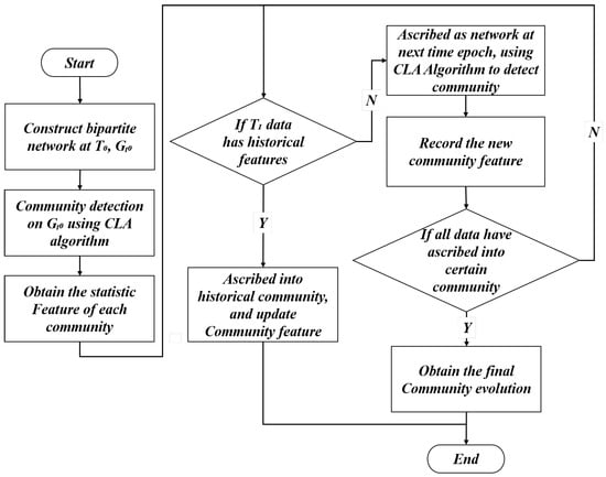
Figure 3. Community structure evolution flowchart of time-varying bipartite network.

The algorithm steps of DyCIAComDet are presented as follows:

Step 1: Segment the entire network G into sub-networks $G_{T_0},G_{T_1},\dots ,G_{T_n}$ with time tags attached.

Step 2: Set i = 0, draw nodes with time tag $T_0$, and construct the corresponding bipartite network $G_{T_0}$; the bipartite network $G_{T_0}$ is used as the initial bipartite network.

Step 3: Apply the CIA algorithm to sub-network $G_{T_0}$, obtain the community partition result, and denote it as $C_1^{T_0},C_2^{T_0},\dots ,C_l^{T_0}$; record their community leadership as $ComL{D}_i^{T_0},i=1,2,\dots ,l$.

Community leadership is defined as the node with the highest weighted degree within the community, as provided in Formula (6).

$$LD=\underset{x\in C}{argmax}\left(\sum _{y\in N\left(x\right)}{w}_{xy}\right)$$

(6)

In Formula (6): x denotes any node (either U-type or V-type) in community C; $N\left(x\right)$ represents the neighbor node list of x (consistent with Formula (1)); ${\sum }_{y\in N\left(x\right)}{w}_{xy}$ calculates the weighted degree of node x; argmax selects the node x with the maximum weighted degree, which is defined as the community leadership node.

The metric Q is traditionally used to evaluate static network community detection results, but it fails to effectively characterize the dynamic evolution of networks. Thus, this paper proposes a novel evaluation metric for dynamic network community evolution. Specifically, the complex network is first sliced into dynamic sub-networks by time. At time $T_{i-1}$, we use the static network community detection method to determine the community result for the network at time epoch $T_{i-1}$. For the network community results from $T_{i-1}$ to $T_i$, the newly added nodes from $T_{i-1}$ to $T_i$ are firstly divided into two parts. The first part consists of nodes that are closely connected to the historical communities at $T_{i-1}$, and their community results are denoted as ${\mathrm{\Omega }}_{T_i-T_{i-1}}^{history}$. The remaining nodes form the second part, and their results are denoted as ${\mathrm{\Omega }}_{T_i-T_{i-1}}^{new}$. Thus, community results from $T_{i-1}$ to $T_i$ can be denoted as $Par{t}_{T_i-T_{i-1}}={\mathrm{\Omega }}_{T_i-T_{i-1}}^{history}+{\mathrm{\Omega }}_{T_i-T_{i-1}}^{new}$.

Step 4: For nodes between time $T_0$ and $T_1$, if nodes have edges with communities found at time $T_0$, the set of nodes is defined as ${\mathrm{\Omega }}_{T_1-T_0}^{history}$. Then, they are assigned into communities at $T_0$, and the community leadership is updated; otherwise, the remaining nodes form a new sub-bipartite network, namely ${\mathrm{\Omega }}_{T_1-T_0}^{new}$.

Step 5: Repeat steps 1–4 between $T_{i-1}$ and $T_i$, and apply the CIA algorithm to the sub-bipartite networks ${\mathrm{\Omega }}_{T_i-T_{i-1}}^{history}$ and ${\mathrm{\Omega }}_{T_i-T_{i-1}}^{new}$; obtain the whole community results of ${\mathrm{\Omega }}_{T_i-T_{i-1}}={\mathrm{\Omega }}_{T_i-T_{i-1}}^{history}+{\mathrm{\Omega }}_{T_i-T_{i-1}}^{new}$, denoted as $C_1^{T_i-T_{i-1}},C_2^{T_i-T_{i-1}},\dots ,C_l^{T_i-T_{i-1}}$, and record the leadership of each community, namely $ComL{D}_i^{T_i-T_{i-1}},i=1,2,\dots ,l$.

The index $Q_{T_i-T_{i-1}}$ for $Par{t}_{\le T_i}$ before $T_i$ is calculated using Formula (7).

$$Q_{\le T_i}={\displaystyle \frac{1}{2m}}\sum _{i=1}^p\sum _{j=1}^q\left[\overline{a_{ij}}-{\displaystyle \frac{k_i{k}_j}{2m}}\right]\left({\eta }_{u_i,v_j}^1+{\eta }_{u_i,v_j}^2+{\eta }_{u_i,v_j}^3\right)\delta (C_{u_i},C_{v_j})$$

(7)

where ${\eta }_{u_i,v_j}^1$ equals 1 if node $u_i$ and node $v_j$ belong to the same community; otherwise, it equals 0. ${\eta }_{u_i,v_j}^2$ equals 1 if node $u_i$ belongs to communities at time epoch $T_{i-1}$, $v_j$ belongs to communities from $T_{i-1}$ to $T_i$ or $u_i$ belongs to communities from $T_{i-1}$ to $T_i$, $v_j$ belongs to communities at time epoch $T_{i-1}$; otherwise, it equals 0. ${\eta }_{u_i,v_j}^3$ equals 1 if both node $u_i$ and $v_j$ belong to communities from $T_{i-1}$ to $T_i$; otherwise, it equals 0. Here, p denotes the total number of U-type nodes ($u_i$) and q the total number of V-type nodes ($v_j$) in the interval $T_{i-1}$ to $T_i$, matching the summation limits in Formulas (7) and (9). Where $Q_{T_i}$ is calculated using Formula (8), while $Q_{T_{i+1}-T_i}$ is calculated using Formula (9).

$$Q_{T_i}={\displaystyle \frac{1}{2m}}\sum _{i,j}[A_{ij}-{\displaystyle \frac{k_i{k}_j}{2m}}]\delta (C_i,C_j)$$

(8)

$$Q_{T_{i+1}-T_i}={\displaystyle \frac{1}{2m}}\sum _{i=1}^p\sum _{j=1}^q\left[\overline{a_{ij}}-{\displaystyle \frac{k_i{k}_j}{2m}}\right]\left({\eta }_{u_i,v_j}^2+{\eta }_{u_i,v_j}^3\right)\delta (C_{u_i},C_{v_j})$$

(9)

Step 6: Merge the existed communities $C_1^{T_i},C_2^{T_i},\dots ,C_l^{T_i}$ and the newfound communities $C_1^{T_{i+1}-T_i},C_2^{T_{i+1}-T_i},\dots ,C_l^{T_{i+1}-T_i}$, the corresponding leadership ${ComLD}_i^{T_{i+1}-T_i},i=1,2,\dots ,l$, and obtain the communities $C_1^{T_{i+1}},C_2^{T_{i+1}},\dots ,C_l^{T_{i+1}}$ and the corresponding leadership ${ComLD}_i^{T_{i+1}}$, $i=1,2,\dots ,l$.

Step 7: Update $i=i+1$ and repeat Step 2–5. Continue this process until one of the following conditions is met: all nodes of the entire network belong to an existing community, or the final time point $T_n$ is reached.The algorithm then terminates.

3.3. BMPS Algorithm for Detecting “Abnormal Alliances”

Section 3 addresses the identification of tax-related anomalous behavior by modeling it as a community evolution problem in dynamic bipartite networks. In Section 4, the paper further addresses the issue of key feature verification for “Abnormal Alliances”. We model this as a frequent pattern mining problem on the sequence database composed of nodes along the evolution paths of “Abnormal Alliances”. The paper proposes the BMPS algorithm for frequent sequence pattern mining, based on concepts such as bitmaps, sequence matrices, sequence prefixes and suffixes, projection matrices, repeated projection matrices, and pattern growth.

BMPS (Bitmap-based PrefixSpan algorithm) is an improved PrefixSpan sequence pattern mining algorithm based on bitmap matrices. Bitmap [25] is a data structure typically used for storing images. Bitmaps are frequently employed for the efficient processing of large-scale binary data. In practical applications, bitmaps are usually stored in the form of image files, such as BMP, PNG, JPEG, and other formats. The advantage of bitmaps is that they can perform efficient bitwise operations, such as AND, OR, XOR, NOT, etc., which is why they are often used in fields of data compression, sorting, deduplication, set operations, and more. In contrast to PrefixSpan, both the sequence data in the sequence database and the projected sequences in the projection database are stored in a two-dimensional sequence matrix.

The flowchart of BMPS is shown in Figure 4.

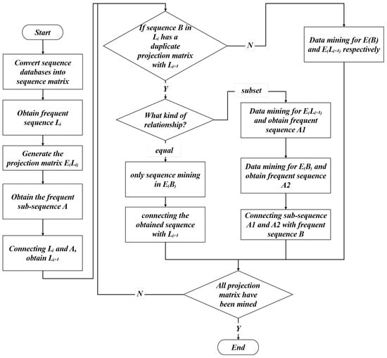
Figure 4. Flowchart of BMPS algorithm.

Step 1: Instead of scanning the original sequence database, the algorithm first scans the sequence matrix E to identify frequent 1-sequence patterns.

For a given sequence database D, if the occurrence frequency of a certain sequence pattern $\alpha$ exceeds the minimum support threshold min_sup, i.e., $Sup\left(\alpha \right)\ge min\_sup$, then the sequence $\alpha$ is called a frequent sequence. The sequence matrix of database D is shown in Table 1, the corresponding bitmap matrix denoted as $\mathit{E}$. Each sequence $d_i$ corresponds to a bitmap matrix are denoted as ${\mathit{E}}_{\left(d_i\right)}$, which is shown in Figure 5.

Table 1. Sequence database.

Sid	Sequence
1	<a(abc)(bc)b(cd)>
2	<(ad)(abc)(bcd)d>
3	<(be)(ae)(c)(d)f>
4	<a(be)(ce)(ac)>

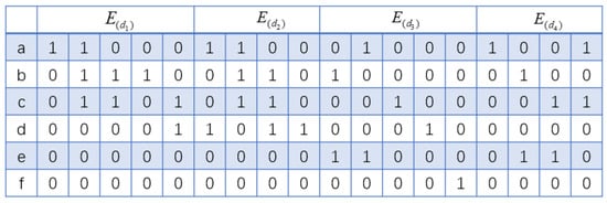
Figure 5. Sequence bitmap matrix.

Taking the sequence database D in Table 1 as an example, its corresponding sequence matrix is shown in Figure 5. D contains four sequences in total, corresponding to the four sequence matrices in Figure 5. D includes six data items: a, b, c, d, e, and f, corresponding to the six rows in Figure 5. When calculating the support of a data item, the algorithm only needs to traverse each row of the matrix. If a ‘1’ appears in a row, the support value of that item is incremented by 1. Then, the algorithm skips the current matrix and continues to traverse the next sequence matrix. Assuming $min\_sup=2$, in {a:4, b:4, c:4, d:3, e:2, f:1} shown in Figure 5, except for item f, all other items are frequent 1-sequence items. By traversing each column of the matrix, we can obtain the item set according to the position value of the sequence. For example, in the second column, only elements a, b, and c have a position value ‘1’; thus, its item set is (abc).

Step 2: Based on the position value of $L_1$ in matrix E, where position usually refers to the location where an element or item appears in the given sequence, the following procedure is performed. Specifically, suppose there is a sequence $\alpha =⟨{\alpha }_1,{\alpha }_2,\dots ,{\alpha }_n⟩$, and there exists an item b and $\mathbf{b}\in {\bigcup }_{j=1}^n{\alpha }_j,{\alpha }_j(\mathbf{b},j)$ represents the position value of item b in the sequence $\alpha$. Matrix E projects and partitions to obtain the projection matrix ${\mathbf{E}}_{\left(L_1\right)}$. The projection matrix ${\mathbf{E}}_{\left(L_1\right)}$, proposed instead of the projection database, is shown as follows. Given a sequence prefix $\alpha$ and a matrix E, the projection matrix of $\alpha$ relative to E, denoted as $E_{\left(\alpha \right)}$, defines the set of position values in E that are greater than the position value of the sequence prefix $\alpha$. Similarly, $E_{(d_i,\alpha )}$ describes the set of position values that are greater than the position value of $\alpha$ in sequence $d_i$.

For example, $\alpha =⟨a\left(b\right)⟩$, the positional values of the sequence prefixes $\alpha$ in E are $d_1(\alpha ,2)$, $d_2(\alpha ,2)$ and $d_4(\alpha ,2)$, respectively. Therefore, scanning all columns after the second column of the matrices corresponding to $d_1$, $d_2$, and $d_4$ in E yields the projection matrix, as shown in Figure 6. Taking $d_1$ as an example, the rules for generating the projection matrix are as follows: the sequence prefix $\alpha$ has a position value of 2 in $d_1$, and the last item of $\alpha$ is b. Therefore, starting from the second column of $E_{\left(d_1\right)}$, traversing vertically, item b is in the second row; thus, all position values before $E_{(d_1,\alpha )}\left[2\right]\left[2\right]$ are 0, which means that the first column of $E_{(d_1,\alpha )}$ is all zeros, namely $E_{(d_1,\alpha )}\left[1\right]\left[2\right]=0$, $E_{(d_1,\alpha )}\left[2\right]\left[2\right]=0$. The values after the second row are the same as those in $E_{\left(d_1\right)}$. The values of the second column and beyond in $E_{\left(d_1\right)}$ are the same as the corresponding values in $E_{(d_1,\alpha )}$.

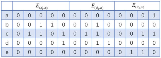
Figure 6. Projection matrix of sequence $\alpha$.

When performing sequence mining, rules for calculating the item support are presented as follows. In Figure 6, by traversing the three matrices where item a is located, there is ‘1’ in $E_{(d_4,\alpha )}$, which is less than the minimum support; by traversing the three matrices where item b is located, there are ‘1’s in both $E_{(d_1,\alpha )}$ and $E_{(d_2,\alpha )}$, and its support is 2. Similarly, the support for all items is obtained as {$⟨\left(a\right)⟩:1,⟨\left(b\right)⟩:2,⟨\left(c\right)⟩:3,⟨\left(d\right)⟩:2,⟨\left(e\right)⟩:1,⟨\left(\_c\right)⟩:2,⟨\left(\_e\right)⟩:$$1\}$. Items with support less than $min\_sup$ = 1 are dropped out; thus, the extensible items are $\left\{⟨\left(b\right)⟩,⟨\left(c\right)⟩,⟨\left(d\right)⟩,⟨\left(\_c\right)⟩\right\}$.

When calculating the item support, it is important to notice the position value of the last item in the prefix sequence, and the items in front of the columns corresponding to the same position value should be prefixed with an underscore “_”, indicating that they belong to the same item set.

Step 3: In the projection matrix $E_{\left(L_1\right)}$, we first mine the frequent subsequences $\alpha$ that satisfy the minimum support. By connecting the frequent 1-sequence patterns $L_1$ with $\alpha$, we obtain frequent 2-sequence patterns. The sequences $L_1$ and $L_2$ satisfy the frequent-sequence relationship due to the equation $CID(L_1,L_2)|E=CID\left(L_2\right)|E$.

The proposed frequent subsequences are shown as follows. Assuming there exist two frequent subsequences, denoted as sequence $\alpha$ and $\beta$, ${CID\left(\alpha \right)|}_D$ represents the set of data records in database D that contain subsequence $\alpha$, and ${CID\left(\beta \right)|}_D$ represents the set of data records in database D that contain subsequence $\beta$. Let ${CID(\alpha ,\beta )|}_D$ denote the set of data records in the database that contain both subsequences $\alpha$ and $\beta$. Therefore, ${CID(\alpha ,\beta )|}_D=CID\left(\alpha \right){{|}_D\bigcap CID\left(\beta \right)|}_D$, and it is said that sequences $\alpha$ and $\beta$ have the frequent-sequence relationship.

If ${\left|CID(\alpha ,\beta )\right|}_D$ < $\left(min\_sup\right)$, then $\alpha$ and $\beta$ do not satisfy the frequent-sequence relationship in database D. This is due to the fact that the number of records containing both $\alpha$ and $\beta$ is less than $min\_sup$. If $mi{n}_{sup}\le {\left|CID(\alpha ,\beta )\right|}_D\le {min\left\{\right|CID\left(\alpha \right)|}_D{,\left|CID\left(\beta \right)\right|}_D\}$, $\alpha$ and $\beta$ satisfy the frequent-sequence relationship in database D.

For example, a sequence database D is shown in Table 1. Suppose min_sup = 2. The data-record set containing $⟨\left(\mathbf{a}\right)⟩$ is ${CID\left(⟨\left(\mathbf{a}\right)⟩\right)|}_D$=$\{1,2,3,4\}$. The data-record set containing $⟨\left(\mathbf{b}\right)⟩$ is ${CID\left(⟨\left(\mathbf{b}\right)⟩\right)|}_D$=$\{1,2,3,4\}$. The data-record set containing both $⟨\left(\mathbf{a}\right)⟩$ and $⟨\left(\mathbf{b}\right)⟩$ is ${CID(⟨\left(\mathbf{a}\right)⟩,⟨\left(\mathbf{b}\right)⟩)|}_D$=$CID(⟨(\mathbf{a})⟩)\bigcap CID(⟨(\mathbf{b})⟩)$=$\{1,2,3,4\}$. The number of records containing both sequences $⟨\left(\mathbf{a}\right)⟩$ and $⟨\left(\mathbf{b}\right)⟩$ is greater than 2; thus, subsequences $⟨\left(\mathbf{a}\right)⟩$ and $⟨\left(\mathbf{b}\right)⟩$ have a frequent-sequence relationship. Also, the data-record set containing the sequence $⟨\left(\mathbf{d}\right)⟩$ is ${CID\left(⟨\left(\mathbf{d}\right)⟩\right)|}_D=\{1,2,3\}$. The data-record set containing sequence $⟨\left(\mathbf{f}\right)⟩$ is ${CID\left(⟨\left(\mathbf{f}\right)⟩\right)|}_D=\{1,2,3\}$. The data-record set containing both $⟨\left(\mathbf{d}\right)⟩$ and $⟨\left(\mathbf{f}\right)⟩$ is ${CID(⟨\left(\mathbf{d}\right)⟩,⟨\left(\mathbf{f}\right)⟩)|}_D=CID\left(⟨\left(\mathbf{d}\right)⟩\right)\bigcap CID(⟨(\mathbf{f})⟩)=\{1,2,3\}$. The number of records containing both subsequences $⟨\left(\mathbf{d}\right)⟩$ and $⟨\left(\mathbf{f}\right)⟩$ is less than 2; thus, the subsequences $⟨\left(\mathbf{d}\right)⟩$ and $⟨\left(\mathbf{f}\right)⟩$ dose do not have a frequent-sequence relationship.

Step 4: According to the Repeated Projection Matrix, there may be three situations with the sequence ${\mathit{L}}_2$ and the frequent 1-sequences $\beta$.

Where Repeated Projection Matrix proposed is shown as follows. Given two frequent subsequences $\alpha$ and $\beta$, assume that the position values of $\alpha$ and $\beta$ are the same within the same sequence, and the count of equal positional values is not less than min_sup. Then, the projection matrix constructed with $\alpha$ and $\beta$ as prefixes duplicates with each other.

Assuming $\alpha$ = $⟨\mathbf{a}\left(\mathbf{b}\right)⟩$, its corresponding projection matrix is shown in Figure 7. Assuming $\beta =⟨\left(\mathbf{b}\right)⟩$, its corresponding projection matrix is also shown in Figure 7. Because $d_1(\alpha ,2)$=$d_1(\beta ,2)$, $d_2(\alpha ,2)$=$d_2(\beta ,2)$, and $d_4(\alpha ,2)$=$d_1(\beta ,2)$ the position values of $\alpha$ and $\beta$ in matrices $d_1$, $d_2$ and $d_4$ are equal. Since the number of equal position values is greater than min_sup, which is 1, it can be observed from Figure 6 and Figure 7 that there are duplicate parts in the projection matrices of $\alpha$ and $\beta$.

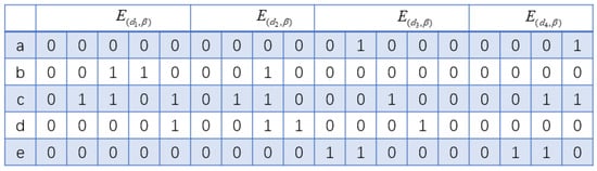
Figure 7. Projection matrix of sequence $\beta$.

The sequence ${\mathit{L}}_2$ includes the following three situations:

Situation (1): The set of position value of $L_2$ in matrix E is the same as the set of position values of $\beta$ in matrix E. In this scenario, there is no need to generate a projection matrix for ${\mathit{L}}_2$; instead, we can directly mine within the projection matrix of $\beta$. By connecting the sub-sequences obtained from $\beta$ with ${\mathit{L}}_2$, we can generate higher-order frequent sequences.

Situation (2): The set of position values of $L_2$ in E is a subset of the position values of $\beta$ in E. Assuming the set of position values for ${\mathit{L}}_2$ in E is $\{j_1,j_2,j_4\}$, and the set of position values for $\beta$ in E is $\{j_1,j_2,j_4\}$, it can be seen from the position value sets that sequence ${\mathit{d}}_3$ contains sequence $\beta$ but not ${\mathit{L}}_2$.

We first perform frequent-sequence mining in the projection matrix of ${\mathit{L}}_2$, and assume that the mined local frequent-sequence items are ${\alpha }^{\prime }=\{{\alpha }_1,{\alpha }_2,{\alpha }_3\}$. Second, we perform mining in the projection matrix of $\beta$ as the prefix, and assume that the mined local frequent sequences are ${\alpha }^{″}=\{{\alpha }_1,{\alpha }_2,{\alpha }_3,{\alpha }_4,{\alpha }_5\}$. Here, we select items contained in sequence ${\mathit{d}}_3$ from ${\alpha }^{″}=\{{\alpha }_1,{\alpha }_2,{\alpha }_3,{\alpha }_4,{\alpha }_5\}$, and assume that the items appearing in d3 are $\{{\alpha }_3,{\alpha }_4\}$, and the result after selection is ${\alpha }^{‴}=\{{\alpha }_1,{\alpha }_2,{\alpha }_5\}$.

A sequence prefix is essentially a subsequence of a sequence. Specifically, suppose we have sequence $\alpha =⟨{\alpha }_1,{\alpha }_2,\dots ,{\alpha }_m⟩$ and sequence $\alpha =⟨{\beta }_1,{\beta }_2,\dots ,{\beta }_n⟩,1\le m\le n$. Sequence $\alpha$ is referred to as a sequence prefix of sequence $\beta$ when the following three conditions are satisfied.

(1) ${\alpha }_i$ ${\beta }_i$; (2)${\alpha }_p\subset {\beta }_p$; and (3) all items in ${\alpha }_p$ appear in the earlier part of ${\beta }_p$.

Example. Suppose $\alpha =⟨\mathbf{a}\mathbf{\left(}\mathbf{abc}\mathbf{\right)}\mathbf{\left(}\mathbf{bc}\mathbf{\right)}\mathbf{\left(}\mathbf{de}\mathbf{\right)}⟩$; then $⟨a\left(a\right)⟩$, $⟨a\left(abc\right)⟩$, $⟨\left(bc\right)\left(b\right)⟩$ are all sequence prefixes of $\alpha$. The projection matrix for the intersection of ${\alpha }^{\prime }$ and ${\alpha }^{‴}$, specifically ${\alpha }_1$ and ${\alpha }_2$, needs to be generated only once, with ${\alpha }_1$ and ${\alpha }_2$ serving as the prefixes. More specifically, the projection matrix for ${\alpha }_1$ and ${\alpha }_2$ is generated during the mining process of $L_2$, and there is no need to regenerate it during the mining process of $\beta$.

Situation (3): The position-value sets of $L_2$ and $\beta$ do not meet situations (1) and (2) in E.

Generate the projection matrix separately and perform the conventional sequence-mining process. The algorithm terminates when all values in the projection matrix are 0 or the support of all items is less than the minimum support threshold.

4. Numerical Experiment

Our numerical experiment is divided into two stages. The first stage involves the identification of community evolution based on a large-scale bipartite network, which is to identify anomalous behavior within large-scale data. The second stage is to search for evidence of anomalous behavior, namely, Abnormal Alliances.

4.1. Comparison of the CIA Algorithm with Other Algorithms

In the following, to validate the effectiveness and reliability of the CIA algorithm proposed in this paper, this study initially constructs artificial bipartite networks through computer simulation for comparative analysis between the CIA algorithm and other algorithms, such as the BRIM algorithm, algorithms based on spectral clustering, and algorithms based on edge clustering coefficients. Then the CIA algorithm is implemented on the Southern Women Dataset and actual tax-related data.

The artificially generated bipartite network in this paper consists of four communities, each containing 10 U-class nodes and 10 V-class nodes. Each node has a degree of 10, where $d_{in}$ represents the number of edges between a node and other nodes within its community, and $d_{out}$ represents the number of edges between a node and nodes outside its community. Meanwhile, the weights between edges within the community are assumed to follow a certain random distribution. The constructed artificial network is shown in Figure 8. When $d_{out}$ = 0, $d_{in}$ = 10 is set, its community structure is very clear in Figure 8. Figure 8a shows the structure of Community 1; Figure 8b shows the structure of Community 2; Figure 8c shows the structure of Community 3; and Figure 8d shows the structure of Community 4. When $d_{out}$ takes the values of 0, 1, 2, 3, and 4, the Normalized Mutual Information (NMI) metrics are calculated for the community partition results obtained by the static CIA algorithm. These results are compared with those from the BRIM algorithm, spectral clustering algorithm, and edge clustering coefficient community detection algorithm, using the real network community structure as a reference. The comparison results are shown in Figure 9. It can be seen from Figure 9 that for different values of $d_{out}$, the NMI values of the CIA algorithm are higher than those of the other three algorithms, indicating that the community partition results obtained by the CIA algorithm are closer to the true community structure of the network. Therefore, the community partitioning results obtained by the CIA algorithm are closer to the true network community structure compared with the other three algorithms under the artificial bipartite network.

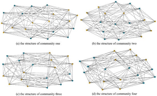
Figure 8. Artificial bipartite network.

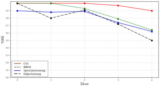
Figure 9. Comparison results of NMI under four algorithms.

In the following section, this paper will validate the effectiveness of the CIA algorithm on real bipartite networks using the publicly available real-world network (Southern Women Dataset), which is a well-known standard bipartite network. It includes 18 woman nodes and 14 activity nodes, with edges representing a woman’s participation in a particular activity, shown in Figure 10.

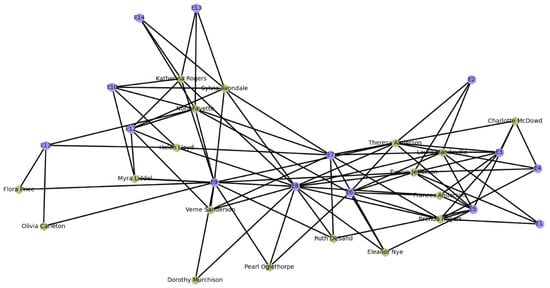
Figure 10. Network of Southern Women.

The community structure partitioned by the CIA algorithm is shown in Figure 11. It can be seen that the CIA algorithm divides the Southern Women into three communities. If the women nodes are sequentially numbered, it can be seen that Community 1 includes six women nodes and activity nodes, including E8, E10, E12, E13, and E14. Community 2 includes five women nodes and activity nodes, including E11 and E9, and Community 3 includes seven women nodes and activity nodes, including E1 to E7.

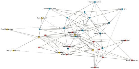
Figure 11. Community structure of Southern Women by CIA algorithm.

From the modularity comparison chart shown in Figure 12, it can be seen that the Q value of the CIA algorithm is significantly higher than the other three algorithms. Comparatively, the Q value of the CIA algorithm has increased by 12.8%, 19.8%, and 8.4% over that of algorithms such as BRIM, spectral clustering, and the edge clustering coefficient, respectively. The community detection algorithm based on spectral clustering requires the number of communities to be known in advance; the parameter is set to 3 due to the three communities identified by the CIA algorithm.

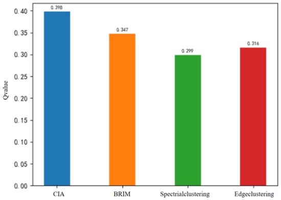
Figure 12. Comparison of the Q value of four community detection algorithms on the Southern Women dataset.

Therefore, the CIA algorithm proposed in this paper outperforms other algorithms in both artificial and real-world network datasets, which shows that the CIA algorithm can identify the true community structure of bipartite networks.

4.2. DyCIAComDet and Anomaly Behavior Detection

DyCIACommDet will be applied to the real large-scale bipartite network composed of taxpayers and tax service providers to perform dynamic community structure detection and evolution trajectory tracking. By identifying the community structures and their evolutionary patterns, potential abnormal tax behaviors can be detected. The dataset includes 280,000 real-name tax transaction records.

Implementation of DyCIAComDet in the taxpayer–tax official network: The CIA algorithm is applied to the sliced taxpayer–tax official network at time $T_0$ for community detection. The resulting community structure is shown in Figure 13 and compared with the community-partitioning results of the BRIM algorithm, algorithms based on spectral clustering, and algorithms based on edge-clustering coefficients, with 18 small communities in total displayed in Figure 13. The comparison of community partitioning performance, based on Q values, is shown in Figure 14. The CIA algorithm achieves a modularity Q value of 0.6134, which represents improvements of 22.7%, 9.6%, and 14.3% compared to the BRIM algorithm, spectral clustering algorithm, and edge clustering coefficient algorithm, respectively. This demonstrates that the CIA algorithm detects a more accurate community structure for the given network.

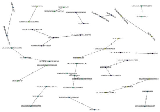
Figure 13. Community structure in the sliced network at $T_0$.

Figure 14. Comparison of Q values of community detection for the sliced network at time $T_0$.

After obtaining the community partitioning of the network at time $T_0$, according to the community evolution algorithm, to facilitate the community detection of the corresponding network in subsequent time slices, this paper records the characteristics of each community at $T_0$, for instance in Table 2, in which the feature sets of the top five communities with the highest number of nodes at time $T_0$ are presented. Then, the data at time $T_1$ is classified based on whether its edges are related to the historical community feature set or not. If a data node has an edge connected to the historical community feature set, the data node is directly assigned to the historical community, and the historical community feature set is updated. Otherwise, a new bipartite network structure at time $T_1$ is constructed, and the CIA algorithm is applied for community detection in the new network at time $T_1$.

Table 2. Characteristics of the community of the network at $T_0$.

Community Name	Feature Set
T0C01	{16101999829, 16101990334}
T0C02	{16101998453, 26100019940}
T0C03	{56101902020}
T0C04	{16101999724}
T0C05	{16101991292}

In the taxpayer–tax-officer network, the data nodes at time $T_1$ are classified according to the following rules: (1) if there is an edge between the taxpayer and the tax officer in the historical community, and either the taxpayer or the tax officer belongs to the feature set of the historical community, then all nodes belong to the historical community; (2) if one of the taxpayers or the tax officer belongs to the feature set of the historical community, then the other node is directly assigned to the historical community; (3) data nodes that do not possess the above two characteristics belong to the network at time $T_1$. The algorithm iterates until $T_n$ when all data belong to a certain community, and the evolution of the entire network stops.

Based on the rules for determining tax-related anomalies, this study proposes two analysis strategies. The first strategy is to identify taxpayers who belong to more than eight different communities at different times and have low transaction weights; these taxpayers can be identified as scalpers. The second strategy is to identify taxpayers who consistently belong to fewer than three fixed communities with high connection weights; these taxpayers can be identified as Abnormal Alliance with tax officers. These transaction data will be further refined and judged in the sequential pattern mining section.

While certain taxpayers (e.g., large state-owned enterprises or corporate headquarters) may naturally exhibit high-frequency interactions with the tax authority as a whole due to operational scale or designated compliance procedures, this study specifically restricts the context to transactions at on-site tax service hall windows rather than the institutional level. Under this constrained setting, if a taxpayer consistently interacts with the same tax officer at the same service window over time, such a pattern constitutes valid grounds for suspicion of anomalous behavior.

As shown in Figure 15, it provides information about partial taxpayer nodes belonging to different communities at various time points. The time range covers from November 2020 to December 2021, totaling 14 time epochs. Vertically, individual nodes belong to different communities at different times, with multiple grids showing different colors. For instance, the taxpayer node 10116101000051727085 belongs to 11 distinct communities over 14 time epochs, and the taxpayer node 10116101000051620205 also belongs to 11 distinct communities in the same period. A large number of similar nodes exist, and these taxpayers can be identified as scalpers. In contrast, other taxpayers consistently belong to only a small number of communities: for example, the taxpayer node 10216101000000248479 always belongs to only one community in all data, and the taxpayer node 10116101000051455599 belongs to only two different communities. These taxpayers have an Abnormal Alliance behavior with tax officers and require further tracking and handling in subsequent steps. Through qualitative review by tax experts, the groups identified in this study are highly suspicious, and some results are highly consistent with historically known violation cases.

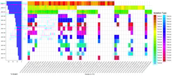
Figure 15. Community evolution.

This paper detects Abnormal Alliances between taxpayers and tax officers by applying the dynamic community detection algorithm, DyCIAComDet, to the real taxpayer–tax officer bipartite network. Furthermore, this paper seeks to verify the Abnormal Alliance behavior between taxpayers and tax officers. The data is then converted into a sequence database and a sequence matrix. The BMPS algorithm is applied for sequence pattern mining to identify frequent sequence abnormal business chains. Subsequently, the taxpayer and tax officer numbers that include these frequent sequences are obtained, thereby verifying the Abnormal Alliance behavior. The transaction dataset used in this study covers a one-year period from November 2020 to November 2021. All records are historical transaction logs collected from the on-site tax service halls; the dataset contains N transactions and was analyzed via monthly time slices to obtain community evolution. Although tax officers may rotate between windows in practice, our analysis does not assume permanent stationarity of taxpayer–tax officer links. Instead, we treat repeated, concentrated interactions over multiple time windows as signals for potential abnormal behavior.

We first analyze the tax business type for each transaction record and then apply the BMPS algorithm to obtain frequent sequence patterns within each business type. The IDs are represented by short characters, as shown in Table 3.

Table 3. Correspondence of ID and code.

Taxpayer id	Code
10216101000000248479	1
10116101010000225684	2
10216101000000116589	3
10216101000000229519	4
10216101000000135342	5
10116101000051770601	6
10116101010000363030	7
16101991299	AA
16101990314	BB
16101998664	CC
16101991332	DD
A00000010200003	a
A00000010200006	b
A00000010200016	c
A00000010200020	d
A00000010200021	e
A00000010200022	f
A00000010200025	g
A00000010200026	h

5. BMPS Performance Analysis

Based on Table 3, due to the vast amount of data, a transaction database corresponding to the business types in Table 3 has been established, along with a transaction database of Abnormal Alliance, as shown in Table 4. We first apply the BMPS algorithm to convert the transaction database of Abnormal Alliance into a sequence database using the following rules. First, the taxpayer ID and the tax officer ID combined form the CID of the sequence database. Second, the business item sets are arranged in the order of occurrence time to form an ordered item set. The resulting sequence database is shown in Table 5. We convert it into the sequence matrix, and the Anomaly Alliance sequence matrix is depicted in Figure 16. Assuming $min\_sup=4$, by scanning the sequence matrix in Figure 16, the support of the 1-sequence is {$⟨\left(a\right)⟩:5$,$⟨\left(b\right)⟩:6$,$⟨\left(c\right)⟩:4$,$⟨\left(d\right)⟩:6$,$⟨\left(e\right)⟩:7$,$⟨\left(f\right)⟩:3$,$⟨\left(g\right)⟩:5$,$⟨\left(h\right)⟩:4$}. All sequences except $⟨\left(f\right)⟩$ satisfy the minimum support threshold. After filtering out the sequence $⟨\left(f\right)⟩$, the remaining sequences are denoted as $L_1$. The projection matrix of $L_1$ is then generated by calculating the position value of $L_1$.

Table 4. Transaction database of Abnormal Alliance.

Taxpayer id	Tax Officer id	Item Set	Date
1	AA	(a)	2020-11
2	BB	(bc)	2020-11
3	CC	(abc)	2020-11
5	DD	(bc)	2020-11
3	CC	(ab)	2020-12
4	AA	(abe)	2020-12
6	CC	(b)	2020-12
1	AA	(bce)	2021-01
7	DD	(de)	2021-01
5	DD	(cef)	2021-01
2	BB	(g)	2021-02
4	AA	(e)	2021-02
6	CC	(ef)	2021-02
1	AA	(de)	2021-03
2	BB	(abc)	2021-03
4	AA	(gh)	2021-04
2	BB	(bcd)	2021-04
6	CC	(degh)	2021-05
5	DD	(fgh)	2021-05
3	CC	(c)	2021-06
7	DD	(de)	2021-06
1	AA	(f)	2021-07
3	CC	(bcd)	2021-07
5	DD	(h)	2021-08
6	CC	(bde)	2021-08
7	DD	(gh)	2021-09
4	AA	(dh)	2021-09
2	BB	(de)	2021-10
7	DD	(a)	2021-10
3	CC	(be)	2021-11
1	AA	(ad)	2021-11
4	AA	(e)	2021-12

Table 5. Sequence database of Abnormal Alliance.

Combined Code (CID)	Seq. Num.	Sequence Database
(1, AA)	$d_1$	<a(bce)(de)f(ad) >
(2, BB)	$d_2$	<(bc)g(abc)(bcd)(de) >
(3, CC)	$d_3$	<(abc)(ab)c(bcd)(be) >
(4, AA)	$d_4$	<(abe)e(gh)(dh)e >
(5, DD)	$d_5$	<(bc)(cef)(fgh)h >
(6, CC)	$d_6$	<b(ef)(degh)(bde) >
(7, DD)	$d_7$	<(de)(de)(gh)a >

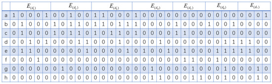
Figure 16. Sequence matrix of Abnormal Alliance.

According to the algorithm in Section 4.2, we first scan the projection matrix. According to the rules for identifying duplicate projection matrices, we discovered that the projection matrices obtained with $⟨\left(c\right)⟩$ as prefix and with $⟨\left(bc\right)⟩$ as prefix duplicate with each other; the projection matrices obtained with $⟨\left(h\right)⟩$ as prefix and with $⟨\left(gh\right)⟩$ as prefix duplicates with each other; and the projection matrices obtained with $⟨\left(e\right)\left(e\right)\left(h\right)⟩$ as a prefix and with $⟨\left(e\right)\left(h\right)⟩$ as prefix duplicate each other. Therefore, these duplicate projection matrices will be mined only once to prevent redundant data mining.

The final frequent sequences obtained with $⟨\left(a\right)⟩$ as prefix are $⟨\left(a\right)\left(d\right)⟩$, $⟨\left(a\right)\left(e\right)⟩$; frequent sequences obtained with $⟨\left(b\right)⟩$ as prefix are $⟨\left(b\right)\left(d\right)⟩$, $⟨\left(b\right)\left(d\right)\left(e\right)⟩$, $⟨\left(b\right)\left(e\right)⟩$, $⟨\left(b\right)\left(g\right)⟩$, $⟨\left(bc\right)\left(e\right)⟩$, $⟨\left(b\right)\left(c\right)⟩$; frequent sequences obtained with $⟨\left(c\right)⟩$ as prefix are $⟨\left(c\right)\left(e\right)⟩$; frequent sequences obtained with $⟨\left(d\right)⟩$ as prefix are $⟨\left(d\right)\left(d\right)⟩$, $⟨\left(d\right)\left(e\right)⟩$, $⟨\left(de\right)⟩$; frequent sequences obtained with $⟨\left(e\right)⟩$ as prefix are $⟨\left(e\right)\left(e\right)⟩$, $⟨\left(e\right)\left(d\right)⟩$, $⟨\left(e\right)\left(h\right)⟩$, $⟨\left(e\right)\left(g\right)⟩$, $⟨\left(e\right)\left(gh\right)⟩$; frequent sequence obtained with $⟨\left(g\right)⟩$ as prefix is $⟨\left(gh\right)⟩$; frequent sequence obtained with $⟨\left(h\right)⟩$ as prefix is $⟨\left(h\right)⟩$.

After obtaining abnormal frequent sequences, the number of abnormal frequent sequences contained in the sequences formed by taxpayers and tax officers is counted, which is significant in further tax investigation. For example, sequence $d_3$ contains 9 abnormal frequent sequences, while sequence $d_4$ contains 17 abnormal frequent sequences. This implies that the suspicion level between taxpayer 3 and tax officer CC is lower than that between taxpayer 4 and tax officer AA. This suspicion level is crucial for tax inspection authorities to prioritize investigations of relevant taxpayers and officials.

In order to assess the performance of the BMPS algorithm in terms of time and space efficiency, we present comparisons of the spatiotemporal efficiency between BMPS and PrefixSpan at different minimum support levels. From Figure 17a, it is evident that the BMPS algorithm outperforms PrefixSpan in terms of time efficiency at different support levels. Especially when min_sup is small, there inevitably exists a huge amount of duplicate projection matrices in the sequence database, leading to a significant difference in time efficiency between BMPS and PrefixSpan. As min_sup increases, the time efficiency gap between BMPS and PrefixSpan narrows, because there are relatively fewer sequences that satisfy the min_sup criterion.

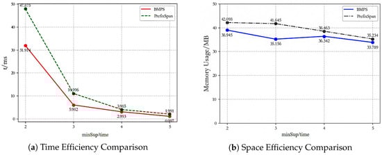
Figure 17. Time and space efficiency comparison between BMPS and PrefixSpan.

From Figure 17b, it is evident that BMPS also surpasses PrefixSpan in terms of space efficiency. In fact, when storing sequences, if the items within the sequence are of character type, at least 1 byte is required. However, if a bitmap matrix is used, only one bit is needed. When the item set contains a large number of items, the space efficiency advantage of BMPS over PrefixSpan becomes more apparent. The reason is that when storing items using a bitmap, there will be fewer 0 values in the columns of the bitmap matrix, preventing it from becoming a sparse matrix; thus, space can be more fully utilized compared to the PrefixSpan algorithm.

To verify the effectiveness of the BMPS algorithm in big data scenarios, all the abnormal alliance data were converted into sequence matrices, and efficiency comparisons with PrefixSpan are shown in Figure 18. It can be found that the BMPS algorithm has significant advantages over the PrefixSpan algorithm in big data scenarios. The reason is that when each item set in the sequences contains large items, using bitmap matrices for storage can save a considerable amount of storage space. Furthermore, avoiding extensive scanning of duplicate projection databases leads to a noticeable improvement in time efficiency.

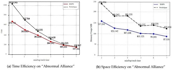
Figure 18. Time and space efficiency comparison on Abnormal Alliance.

From Figure 18a, it can be seen that when min_sup is 2 and 3, the BMPS algorithm improves time efficiency by 34.8% and 28.3%, respectively, compared with the PrefixSpan algorithm, which demonstrates that using bitmap storage and position values to reduce large scanning of duplicate projection matrices can greatly enhance the algorithm’s time efficiency. When min_sup is 4, 5, 6, and 7, the time efficiency improvement of BMPS over PrefixSpan decreases, suggesting that there are fewer sequences satisfying the min_sup threshold, and the depth of sequences obtained under BMPS and PrefixSpan is essentially the same. From Figure 18b, we can see that under different min_sup thresholds, BMPS saves more space than PrefixSpan. When min_sup is 4, BMPS saves the most space, which amounts to 35.3%; when min_sup is 5, it saves the least, which is 25.2%. This demonstrates the high applicability of bitmap storage in scenarios where item set sequences contain a huge number of items.

6. Conclusions and Discussion

Targeting the hard problem of mining and verifying potential abnormal group behavior in a large-scale tax-related bipartite network composed of taxpayers and tax officials, this paper proposes a two-module framework. The framework includes two modules: abnormal group behavior identification and key feature verification.

Module one innovatively proposes the dynamic community structure identification algorithm on a large-scale time-varying bipartite network, namely DyCIAcomDet, based on indicators including cohesion, integration, and leadership. Performance comparisons were conducted on artificially generated data, small-scale public data, namely Southern Women, and large-scale real tax-related data, which validates the efficiency and superiority DyCIAcomDet.

Module two focuses on the verification of key features under Abnormal Alliance’s behavior. It first proposes the frequent sequence mining algorithm BMPS. This algorithm is based on the concepts of bitmap matrices, bit sequence matrices, projection matrices, and duplicate projection matrices. BMPS addresses the problem of low spatiotemporal efficiency in big data scenarios caused by repeated scanning of duplicate projection matrices in the PrefixSpan algorithm.

It should be noted that the coefficient 1.87 is optimized based on specific datasets and may be overfit to them, and its effectiveness in extremely sparse or scale-free networks requires further verification. In addition, the algorithm may carry an inherent bias of equating high-frequency interaction with fraudulent collusion. The fixed contacts required in legitimate business scenarios could thus be mislabeled, constituting an ethical risk that should be prioritized in practical applications.

References

- Wen, D.; Yuan, Y.; Li, X.-R. Artificial Societies, Computational Experiments, and Parallel Systems: An Investigation on a Computational Theory for Complex Socioeconomic Systems. IEEE Trans. Serv. Comput. 2013, 6, 177–185. [Google Scholar] [CrossRef]
- Muradyan, A. The Future of Tax Administration. Belt Road Initiat. Tax J. 2024, 5, 15–19. [Google Scholar]
- Zhang, C.; Deng, L. Microbial Community Analysis based on Bipartite Graph Clustering of Metabolic Network. J. Phys. Conf. Ser. 2021, 1828, 012092. [Google Scholar] [CrossRef]
- Cui, Y.; Wang, X. Uncovering overlapping community structures by the key bi-community and intimate degree in bipartite networks. Phys. A 2014, 407, 7–14. [Google Scholar] [CrossRef]
- Liu, D.; Jin, D.; He, D.; Huang, J.; Yang, J.; Yang, B. Community Mining in Complex Networks. J. Comput. Res. Dev. 2013, 50, 2140–2154. [Google Scholar]
- Li, L.; Liu, X.; Wang, H.; Wang, X. (Eds.) Mathematical Foundations and Applications of Big Data; University of Electronic Science and Technology of China Press: Chengdu, China, 2024; ISBN 978-7-5770-0867-7. [Google Scholar]
- Himmelstein, D.S.; Baranzini, S.E. Heterogeneous Network Edge Prediction: A Data Integration Approach to Prioritize Disease-Associated Genes. PLoS Comput. Biol. 2015, 11, e1004259. [Google Scholar] [CrossRef] [PubMed]
- Li, M.; Jiang, Y.; Di, Z. Characterizing the importance of nodes with information feedback in multilayer networks. Inf. Process. Manag. 2023, 60, 103344. [Google Scholar] [CrossRef]
- Rachamadugu, S.; Pushphavathi, T. A Comparative Analysis of Community Detection Agglomerative Technique Algorithms and Metrics on Citation Network. Ann. Emerg. Technol. Comput. 2023, 7, 1–13. [Google Scholar] [CrossRef]
- An, P.; Zhou, J.; Li, H.; Sun, B.; Shi, Y. The evolutionary similarity of the co-shareholder relationship network from institutional and non-institutional shareholder perspectives. Phys. A 2018, 503, 439–450. [Google Scholar] [CrossRef]
- Li, J.; Ren, D.; Feng, X.; Zhang, Y. Network of listed companies based on common shareholders and the prediction of market volatility. Phys. A 2016, 462, 508–521. [Google Scholar] [CrossRef]
- Moon, S.; Bergey, P.K.; Iacobucci, D. Dynamic Effects among Movie Ratings, Movie Revenues, and Viewer Satisfaction. J. Mark. 2010, 74, 108–121. [Google Scholar] [CrossRef]
- Wang, M.; Chen, W.; Huang, Y.; Contractor, N.S.; Fu, Y. A Multidimensional Network Approach for Modeling Customer-Product Relations in Engineering Design. In Proceedings of the 27th International Conference on Design Theory and Methodology (ASME IDETC/CIE), Boston, MA, USA, 2–5 August 2015; p. V007T06A044. [Google Scholar] [CrossRef]
- Hu, K.; Xiang, J.; Yu, Y.-X.; Tang, L.; Xiang, Q.; Li, J.-M.; Tang, Y.-H.; Chen, Y.-J.; Zhang, Y. Significance-based multi-scale method for network community detection and its application in disease-gene prediction. PLoS ONE 2020, 15, e0227244. [Google Scholar] [CrossRef] [PubMed]
- Guimerà, R.; Sales-Pardo, M.; Amaral, L.A.N. Module identification in bipartite and directed networks. Phys. Rev. E 2007, 76, 036102. [Google Scholar] [CrossRef] [PubMed]
- Barber, M.J. Modularity and community detection in bipartite networks. Phys. Rev. E 2007, 76, 066102. [Google Scholar] [CrossRef] [PubMed]
- Murata, T. Detecting Communities from Bipartite Networks Based on Bipartite Modularities. In Proceedings of the 2009 International Conference on Computational Science and Engineering (CSE), Washington, DC, USA, 29–31 August 2009; Volume 4, pp. 50–57. [Google Scholar] [CrossRef]
- Liu, X.; Murata, T. How Does Label Propagation Algorithm Work in Bipartite Networks? In Proceedings of the 2009 IEEE/WIC/ACM International Joint Conference on Web Intelligence and Intelligent Agent Technology (WI-IAT), Washington, DC, USA, 15–18 September 2009; Volume 3, pp. 5–8. [Google Scholar] [CrossRef]
- Raghavan, U.N.; Albert, R.; Kumara, S. Near linear time algorithm to detect community structures in large-scale networks. Phys. Rev. E 2007, 76, 036106. [Google Scholar] [CrossRef] [PubMed]
- Li, Z.; Wang, R.-S.; Zhang, S.; Zhang, X.-S. Quantitative function and algorithm for community detection in bipartite networks. Inf. Sci. 2016, 367–368, 874–889. [Google Scholar] [CrossRef]
- Chang, F.; Zhang, B.; Zhao, Y.; Wu, S.; Zou, G.; Niu, S. Overlapping Community Detection in Bipartite Networks using a Micro-bipartite Network Model: Bi-EgoNet. J. Intell. Fuzzy Syst. 2019, 37, 7965–7976. [Google Scholar] [CrossRef]
- Wang, Y.; Di, Z.; Fan, Y. Comparative Definition of Community in Bipartite Network. Complex Syst. Complex. Sci. 2009, 6, 40–44. [Google Scholar]
- Agrawal, R.; Srikant, R. Mining sequential patterns. In Proceedings of the Eleventh International Conference on Data Engineering (ICDE), Taipei, Taiwan, 6–10 March 1995; pp. 3–14. [Google Scholar] [CrossRef]
- Srikant, R.; Agrawal, R. Mining sequential patterns: Generalizations and performance improvements. In Advances in Database Technology—EDBT ’96; Apers, P., Bouzeghoub, M., Gardarin, G., Eds.; Springer: Berlin/Heidelberg, Germany, 1996; pp. 1–17. ISBN 978-3-540-49943-5. [Google Scholar]
- Ayres, J.; Flannick, J.; Gehrke, J.; Yiu, T. Sequential Pattern mining using a bitmap representation. In Proceedings of the Eighth ACM SIGKDD International Conference on Knowledge Discovery and Data Mining (KDD), Edmonton, AB, Canada, 23–26 July 2002; pp. 429–435. [Google Scholar] [CrossRef]
- Han, J.; Pei, J.; Yin, Y. Mining frequent patterns without candidate generation. SIGMOD Rec. 2000, 29, 1–12. [Google Scholar] [CrossRef]
- Han, J.; Pei, J.; Mortazavi-Asl, B.; Chen, Q.; Dayal, U.; Hsu, M.-C. FreeSpan: Frequent pattern-projected sequential pattern mining. In Proceedings of the Sixth ACM SIGKDD International Conference on Knowledge Discovery and Data Mining (KDD), Boston, MA, USA, 20–23 August 2000; pp. 355–359, ISBN 1581132336. [Google Scholar]
- Pei, J.; Han, J.; Mortazavi-Asl, B.; Pinto, H.; Chen, Q.; Dayal, U.; Hsu, M.-C. PrefixSpan: Mining sequential patterns efficiently by prefix-projected pattern growth. In Proceedings of the 17th International Conference on Data Engineering (ICDE), Washington, DC, USA, 2–6 April 2001; pp. 215–224. [Google Scholar] [CrossRef]
- Wang, F.; Zhang, M.; Yan, X. Practice of Creating HBASE Secondary Index Based on Bitmap Technology. Inf. Commun. Technol. 2021, 3, 78–82. [Google Scholar]
Disclaimer/Publisher’s Note: The statements, opinions and data contained in all publications are solely those of the individual author(s) and contributor(s) and not of MDPI and/or the editor(s). MDPI and/or the editor(s) disclaim responsibility for any injury to people or property resulting from any ideas, methods, instructions or products referred to in the content. |
© 2025 by the authors. Licensee MDPI, Basel, Switzerland. This article is an open access article distributed under the terms and conditions of the Creative Commons Attribution (CC BY) license (https://creativecommons.org/licenses/by/4.0/).