Article

Generative Models Utilizing Padding Can Efficiently Integrate and Generate Multi-Omics Data

1
Korea AI Center for Drug Discovery and Development, Korea Pharmaceutical and Bio-Pharma Manufacturers Association, Seoul 06666, Republic of Korea
2
Tumor Microenvironment Branch, Division of Cancer Biology, Research Institute, National Cancer Center, Goyang 10408, Republic of Korea
3
Department of Cancer Biomedical Science, NCC-GCSP, National Cancer Center, Goyang 10408, Republic of Korea
4
Celemics, Inc., Seoul 08506, Republic of Korea
5
Department of Orthopaedic Surgery, Hospital, National Cancer Center, Goyang 10408, Republic of Korea
*
Author to whom correspondence should be addressed.
AI 2024, 5(3), 1614-1632; https://doi.org/10.3390/ai5030078
Submission received: 11 July 2024 / Revised: 27 August 2024 / Accepted: 2 September 2024 / Published: 5 September 2024

Abstract

:
Technological advances in information-processing capacity have enabled integrated analyses (multi-omics) of different omics data types, improving target discovery and clinical diagnosis. This study proposes novel artificial intelligence (AI) learning strategies for incomplete datasets, common in omics research. The model comprises (1) a multi-omics generative model based on a variational auto-encoder that learns tumor genetic patterns based on different omics data types and (2) an expanded classification model that predicts cancer phenotypes. Padding was applied to replace missing data with virtual data. The embedding data generated by the model accurately classified cancer phenotypes, addressing the class imbalance issue (weighted F1 score: cancer type > 0.95, primary site > 0.92, sample type > 0.97). The classification performance was maintained in the absence of omics data, and the virtual data resembled actual omics data (cosine similarity mRNA gene expression > 0.96, mRNA isoform expression > 0.95, DNA methylation > 0.96). Meanwhile, in the presence of omics data, high-quality, non-existent omics data were generated (cosine similarity mRNA gene expression: 0.9702, mRNA isoform expression: 0.9546, DNA methylation: 0.9687). This model can effectively classify cancer phenotypes based on incomplete omics data with data sparsity robustness, generating omics data through deep learning and enabling precision medicine.

1. Introduction

Omics is the study of comprehensive datasets from a wide spectrum of biological materials, including genomes, transcriptomes, and proteomes. As such, omics is crucial in clinical diagnosis, drug development, and precision medicine, as it deals with the discovery of disease-specific genetic information and structural variation. With advances in high-throughput technologies, such as the BeadChip array and next-generation sequencing technologies, gene expression, isoform expression, and DNA methylation data have been mass-produced [1,2]. Although these omics data contain various pieces of information, certain sets exhibit association [3,4]. For instance, DNA methylation is associated with gene expression, and gene expression is associated with protein levels [5].
While initial omics analyses utilized a single data type [6,7,8,9,10], the advancement of computer technology and subsequent rapid progress in information-processing capacity has enabled the integrated analysis of various omics data (multi-omics), from genomes and transcriptomes to proteomes [11,12,13]. Indeed, multi-omics is an emerging strategy to develop various models for target discovery, clinical diagnosis, disease subtyping, etc. [13,14,15,16,17,18,19,20,21,22,23,24,25].
Advanced technologies, such as machine learning (ML), have shown promise for application in multi-omics research [26,27]. ML enables the consideration of interactions across diverse datasets, allowing for the utilization of a broader range of information and enabling higher levels of accuracy. In this context, applying ML to multi-omics research offers opportunities to gain profound insights into diseases by analyzing interactions among omics from various perspectives. Active research is focused on multi-omics analyses with ML in brain disease, diabetes, cancer, and cardiovascular disease [28,29,30,31]. Nevertheless, the numerous dimensions against the number of samples in multi-omics analyses negatively impact ML [1]. Up to 20,000 protein-coding genes and 60,000 long non-coding RNAs have been identified based on Gencode 7 [32]. In addition, 96% of 480 K CpG sites can be analyzed based on the most widely used data platform for DNA methylation [33]. Using such high-dimensional data in ML could lead to overfitting (i.e., the curse of dimensionality) and reduce model performance [16].
To resolve this issue, dimensionality reduction based on domain knowledge, dimensionality reduction algorithms, and deep learning generative models are typically used in ML [34,35,36,37]. In particular, generative models learn how to approximate the distribution of data. The variational auto-encoder (VAE) [38] is a generative model that extracts features of input data, stores them in latent vectors, and generates new data similar to the input data through latent vectors. Given that latent vectors can describe the input data well, dimensionality reduction based on VAE has been applied to various omics analyses [37,39].
Despite showing promise, VAE-based models have limitations. First, in multi-omics analyses, missing data from a given sample can prevent its use in learning, and a reduced sample size can lead to poor performance of learning algorithms. However, obtaining sufficient sample sizes is challenging in real-world scenarios due to difficulties in patient enrollment. Second, when omics data collected from different institutions vary in type, the performance of models is limited due to poor data integration, as all samples must possess the required feature values demanded by the ML model. Consequently, related studies have utilized large-scale open data, such as The Cancer Genome Atlas (TCGA)’s Pan-Cancer Atlas (PanCan) [40]. However, when only a portion of omics data types are available, such as in the prospectively collected data from the Korean Sarcoma Biobank Innovation Consortium (SBIC), existing integrated analytical methods cannot be applied. Therefore, a method for efficiently integrating various omics data sources while preserving the independent features of each aspect is necessary [41].
Integrating incomplete and complete data for analysis can lead to increased availability of samples and thus expectations of improved performance. Cao and Gao [42] proposed GLUE (Graph-Linked Unified Embedding), a modular framework for integrating unpaired single-cell multi-omics data and inferring regulatory interactions simultaneously. By leveraging biological knowledge to explicitly model inter-layer regulatory interactions connecting hierarchical functional spaces with a knowledge-based graph (“guidance graph”), this model integrates and analyzes omics data from various sources, effectively capturing diverse cell states. Du et al. [43] used missing masks to learn conditional distributions of unseen patterns and features. By explicitly learning the conditional distributions of specific masked features (or forms) when unmasked features (or modalities) were provided, they conducted an integrated analysis of omics data and achieved high accuracy in cross-domain translation tasks.
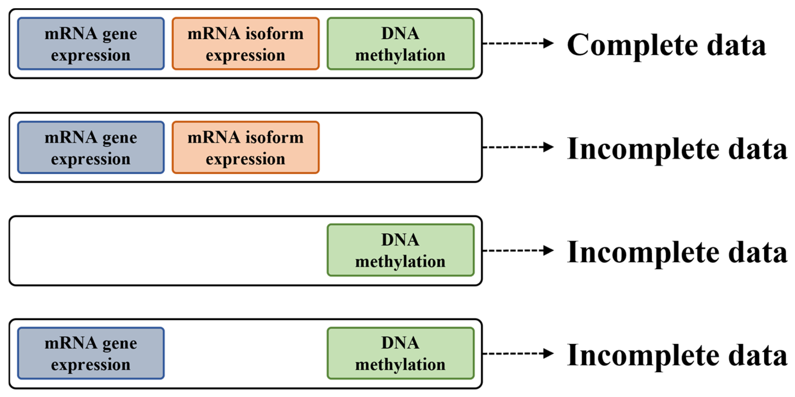
This study proposes a novel artificial intelligence (AI) model and learning strategies that can effectively utilize incomplete data frequently found in omics datasets for pan-cancer. In this paper, “complete data” refers to that in which all omics data to be utilized exist. For example, when using mRNA gene expression, mRNA isoform expression, and DNA methylation in multi-omics, the case where all three omics data types exist can be called “complete data”. “Incomplete data” refers to data in which some of the omics data to be utilized are missing. In the same multi-omics example as that used for “complete data”, a case in which DNA methylation data do not exist can be referred to as “incomplete data” (Figure 1).
Thus, within the current study, a single AI model capable of handling complete and incomplete data was designed. To allow for the input of samples with missing omics data in the AI model, we selected the padding strategy to replace missing omics data with 0 (Figure 2). For the omics data (mRNA gene expression, mRNA isoform expression, and DNA methylation), samples with all column (gene symbol) values of 0 did not appear in the actual data distribution (Figures S1–S3). It was thus hypothesized that the AI model would recognize such values in the absence of actual data. Additionally, an AI model was designed to infer missing omics data by learning from the partial input omics data. If the omics data generated for the missing data are similar to the actual values, they can replace single data points that do not exist in multi-omics. In addition, if the generated omics data are used for embedding, the resulting distribution will resemble that of the embedding based on actual data. Finally, the utility of the novel approach against previous methods that disallow the use of incomplete data was validated. To this end, a phenotype prediction function was added to the model, and its performance was evaluated.
The proposed model consists of two key components: a VAE-based multi-omics generative model that can learn the genetic patterns of tumors based on different omics data and an expanded classification model that can predict cancer phenotypes. Comprehensive analyses validated the versatility of the model. In particular, data for a few samples or omics data with missing parts, such as in the Korean SBIC data, can be applied for learning. Furthermore, the newly developed method enables the generation of virtual genomic data that resemble actual genomic data based on inferences of missing omics data.

2. Materials and Methods

2.1. Data Source

2.1.1. TCGA Pan-Cancer (PanCan)

The open TCGA PanCan database integrates mutation data for over 10,000 samples of 33 cancer types. The TCGA PanCan data are widely used in precision medicine research, including in training AI models to discover cancer diagnostic markers.
This study used biospecimens and data from the SBIC for Biomedical and Healthcare Research. All PanCan data were downloaded from the University of California Santa Cruz (UCSC) Xena platform [44]. Data were integrated after each of the final data preprocessing sets, and the max–min normalization was applied to obtain values between 0 and 1.

2.1.2. Korea Biobank Network-SBIC

The SBIC, as part of the Korea Biobank Project, aims to construct a national registry to support research on rare cancers and promote translational research by integrating and accumulating data for various human-related materials and subsequently generating mutation data for sarcoma (SARC). The SBIC data were used in this study in collaboration with the consortium project to construct the Korean Sarcoma Biobank.
For use as the input in the proposed model, the SBIC data, as with the PanCan data, were integrated after each of the final data preprocessing steps and the max–min normalization to obtain values between 0 and 1.

2.2. Data Types

2.2.1. mRNA Gene Expression Data

Gene expression is the process by which information from a gene is used to synthesize a functional gene product that produces end-products, namely protein or non-coding RNA, ultimately affecting cell phenotype. Many studies employ gene expression data to assess tumor states and for molecular profiling [37,45]. The PanCan mRNA gene expression data contains 60,498 gene symbols related to 10,535 samples; the SBIC mRNA gene expression data contains 25,268 gene symbols pertaining to 45 samples. In this study, we only included 10,496 samples with phenotype data in the case of PanCan, as the proposed model performs a supervised learning task for the classification of cancer phenotypes. In addition, to amalgamate the PanCan and SBIC data, new integrated data were generated utilizing 23,191 gene symbols shared between the two datasets. The fragments per kilobase of transcript per million (FPKM) values for the respective data were log-transformed using RNA-seq by expectation maximization (RSEM; log2(FPKM + 0.001)).

2.2.2. mRNA Isoform Expression Data

Gene isoforms are mRNAs produced from the same locus with distinct transcription start sites, protein-coding DNA sequences, and/or untranslated regions that can alter gene function [46]. Recent studies have shown that several gene isoforms directly function in tumor transformation and growth [47]. The PanCan mRNA isoform expression data contain 197,045 gene symbols for 10,535 samples, and the SBIC mRNA isoform expression data contain 25,268 gene symbols for 45 samples. From the PanCan data, only 10,495 samples with phenotype data were included, and an additional 23,191 gene symbols shared with the SBIC dataset were included. The FPKM values for the respective data were log-transformed using RSEM (log2(FPKM + 0.001)).

2.2.3. DNA Methylation Data

DNA methylation is an epigenetic mechanism in which a methyl group is transferred to the C5 position of cytosine to form 5-methylcytosine. DNA methylation regulates gene expression by recruiting proteins involved in gene inhibition or by inhibiting the binding of transcription factors to DNA. Given that DNA methylation in a specific region can be directly related to oncogene expression, it is currently widely studied as a major indicator and target of cancer [48]. The PanCan DNA methylation data contain 396,065 methylation IDs for 9639 samples; the SBIC data do not include DNA methylation data. From the PanCan data, samples other than the 9602 with phenotype data were excluded. In addition, the methylation IDs other than the 269,273 with a NaN value were excluded. The respective data were downloaded from UCSC Xena. The DNA methylation data were reformatted using the metadata from the previous methylation ID to a gene-symbol-based structure. The beta value was the mean value across the methylation IDs of each gene symbol.

2.2.4. Phenotype Data

The phenotype data comprised the combination (11,369 cases) of the samples in the PanCan and SBIC datasets, including various parameters from retrospective data, e.g., cancer type, sample type, primary site, tumor event, sex, race, and stage. The phenotypes used in the model learning and result analysis were cancer type, primary site, and sample type.
The cancer types investigated were adrenocortical carcinoma, bladder urothelial carcinoma, breast invasive carcinoma (BRCA), cervical squamous cell carcinoma, endocervical adenocarcinoma, cholangiocarcinoma, colon adenocarcinoma, lymphoid neoplasm diffuse large B-cell lymphoma, esophageal carcinoma, glioblastoma multiforme, head and neck squamous cell carcinoma, kidney chromophobe, kidney renal clear cell carcinoma (KIRC), kidney renal papillary cell carcinoma, acute myeloid leukemia, brain lower grade glioma, liver hepatocellular carcinoma, lung adenocarcinoma, lung squamous cell carcinoma, mesothelioma, ovarian serous cystadenocarcinoma, pancreatic adenocarcinoma, pheochromocytoma and paraganglioma, prostate adenocarcinoma, rectum adenocarcinoma, SARC, skin cutaneous melanoma, stomach adenocarcinoma (STAD), testicular germ cell tumors, thyroid carcinoma, thymoma, uterine corpus endometrial carcinoma (UCEC), uterine carcinosarcoma, and uveal melanoma.
The primary sites investigated were adrenal gland, bile duct and gallbladder, bladder, bone marrow, brain, breast, cardia, cerebrum, cervix uteri, cortex of adrenal gland, esophagus, eye, head and neck, intestine, kidney, liver, lung, lymph nodes, oral, ovary, pancreas, peritoneum, pleura, prostate gland, skin, stomach, subcutaneous and soft tissues, testis, thymus, thyroid gland, tongue, and uteri.
The sample types investigated were additional–new primary, metastatic, primary blood-derived cancer–peripheral blood, primary tumor, recurrent tumor, and solid tissue normal types.

2.3. Padding

Three types of omics data were applied: mRNA gene expression, mRNA isoform expression, and DNA methylation data. Some samples exhibited only one or two types of omics data (Table 1).
The padding strategy was applied for data processing and inferences on each sample. For each omics data sample, the padding set was expressed as the difference between the union of all omics data samples and the set of each omics data sample. The padding value was unified as 0. The size of the sample union for all genomes was 11,369, and padding data were generated for the expression of 1034 genes and 1035 isoforms and beta values for 1973 methylation sites.

2.4. Model Structure

The proposed model was structured based on semi-supervised learning with the addition of a predictive model to the generative model. The multi-omics generative model identifies tumor genetic patterns based on several omics data types for embedding in a low-dimensional vector. The expanded classification model makes inferences on the phenotype of the given cancer type. In addition, for samples with one or more missing omics data types, padding is added for the flexible generation of embedding, even in the absence of specific omics data in reference to others.

2.5. Implementation Details

The proposed model was designed using PyTorch Lightning (version 1.6.3) [49], which provides an advanced interface for PyTorch (version 1.11.0) [50]. Overall, the model comprises linear neural networks with the rectified linear unit activation function and layer normalization. The hyperparameters were set to their optimal values within the search range (Table 2).
The multi-omics generative model is structured based on a modified VAE with three layers: the Expanded Encoder, the Concat Layer, and the Expanded Decoder. The Expanded Encoder layer comprises M encoders. The size of the input data for each encoder is equivalent to the number of each omics data point, while an encoder is composed of layers that create vectors with sizes of 1000, 500, and 100. Here, M is the number of omics data types used in learning. Two roles are assigned to the Concat Layer. First, it concatenates the vectors generated by the Expanded Encoder layer into a single vector with the output of the final encoding vector. Second, it realizes the reparameterization of the VAE with the output of the latent vector. The size of the latent vector, as the final output of the respective layer, is 100. The Expanded Decoder layer comprises a layer that takes the latent vector input to generate vectors with sizes of 500 or 1000 and a layer that generates vectors with sizes that correspond to the features of each omics data type. The final output of each decoder layer serves to reconstruct the original omics data.
The expanded classification model comprises several models, each with a single-layer structure. The embedding data are used to predict the phenotype data, and the learning outcome is transferred to the generative model.

2.6. Learning Strategies

Three criteria should be met for the proposed model to attempt learning. First, the model should perform even in the absence of certain omics data in the learning sample. Second, the model should be able to make inferences even in cases of missing omics data. Third, the concurrent use of incomplete data should contribute to enhanced performance. For this, the parameter optimization steps in the multi-omics generative model and expanded classification model were defined in the learning strategies.

2.6.1. Multi-Omics Generative Model

The multi-omics generative model has a VAE-based design. The VAE is a deep neural network that can detect manifolds in high-dimension raw data to generate useful features for other operations, such as classification and regression. In the VAE structure, the input data x pass through the encoder to produce the latent vector z with the feature data, and the vector z passes through the decoder, generating similar output data to the input data x. Loss in the multi-omics generative model, as with general loss in VAE structures, is based on the union of the reconstruction loss indicating the difference in the input data x from the data g restructured by the decoder and the regularization loss that controls the latent vector z after sampling by reparameterization to follow the normal distribution.
The learning strategies vary between the multi-omics generative model and general VAEs. The former applies the padding technique to utilize as much information as possible, even in the absence of certain omics data. With padding, missing data are assigned values of 0, and the respective reconstruction may limit model learning. Hence, loss attributed to padding was excluded in the calculation of the reconstruction loss by using a filter that differentiated between actual data and padding data. In addition, the final loss from the expanded classification model with the inferences on cancer phenotypes was considered so that the reconstruction of the original data could incorporate the learning outcome for phenotype data.

2.6.2. Expansion of the Classification Model

The expanded classification model comprises three models that predict three parameters (cancer type, primary site, and sample type) with a linear single-layer structure in each model. Each classification model receives the latent vector from the multi-omics generative model as the input to predict the phenotype. Instead of the categorical cross-entropy loss commonly used for general classification models, we calculated the focal loss [51], which can improve the class imbalance issue. The final loss of the expanded classification model was calculated as the sum of the losses of each classification model.

2.7. Performance Evaluation

The classification label used in the proposed model was “phenotypes with a class imbalance problem”, i.e., substantial differences in the amount of data among classes. Hence, the F1 score for each class was calculated, and the weighted mean was obtained according to the data percentage per class to estimate the total F1 score (weighted F1 score) to ensure the accurate evaluation of model performance. The weighted F1 score was calculated using Scikit-learn [52]. In addition, to verify that the proposed model could be used to make inferences in cases of missing omics data, the mean absolute error was used, and certain omics data were replaced with padding data and compared with the restructured data for samples with complete omics data. We used the Scikit-learn library for t-SNE calculations and the Bokeh [53] library for visualization.

3. Results

3.1. Phenotype Classification Task

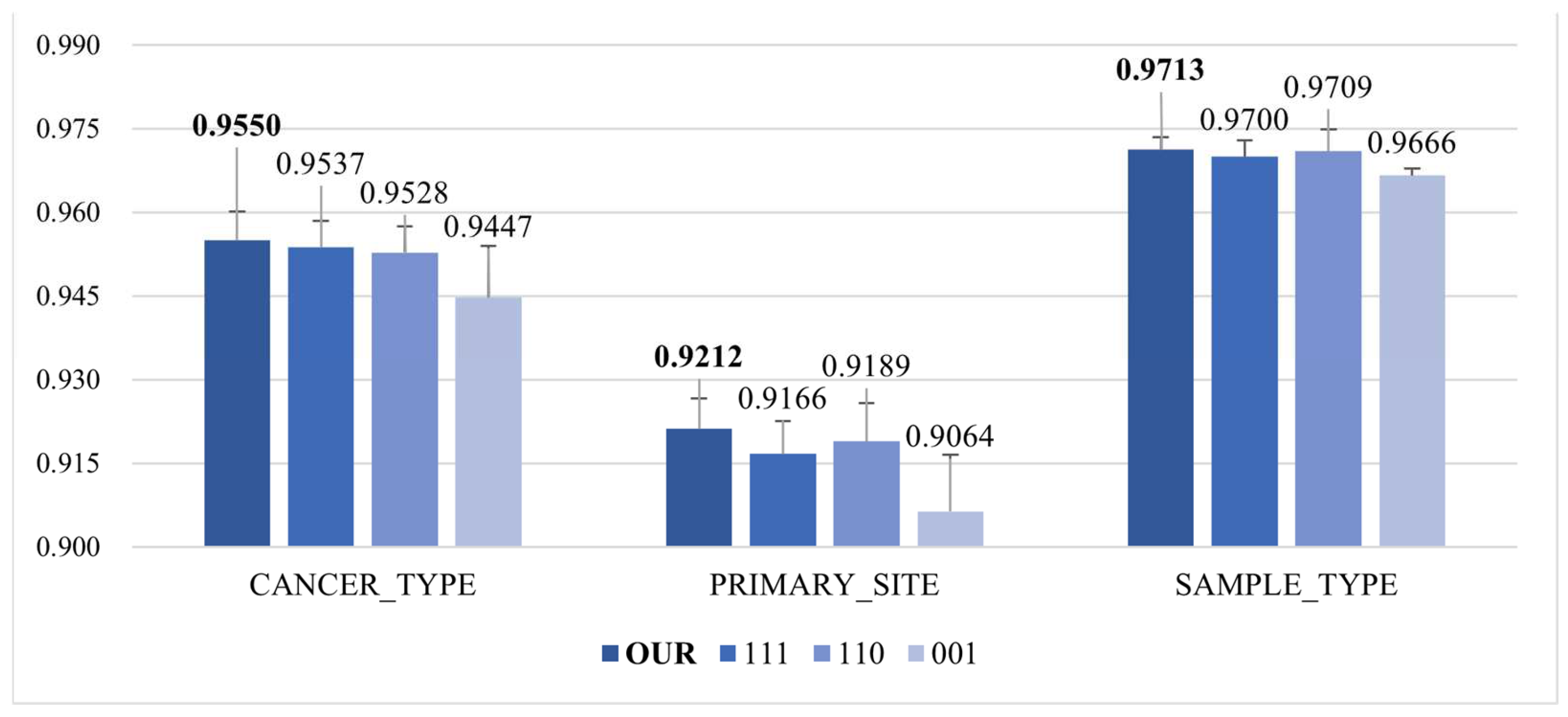
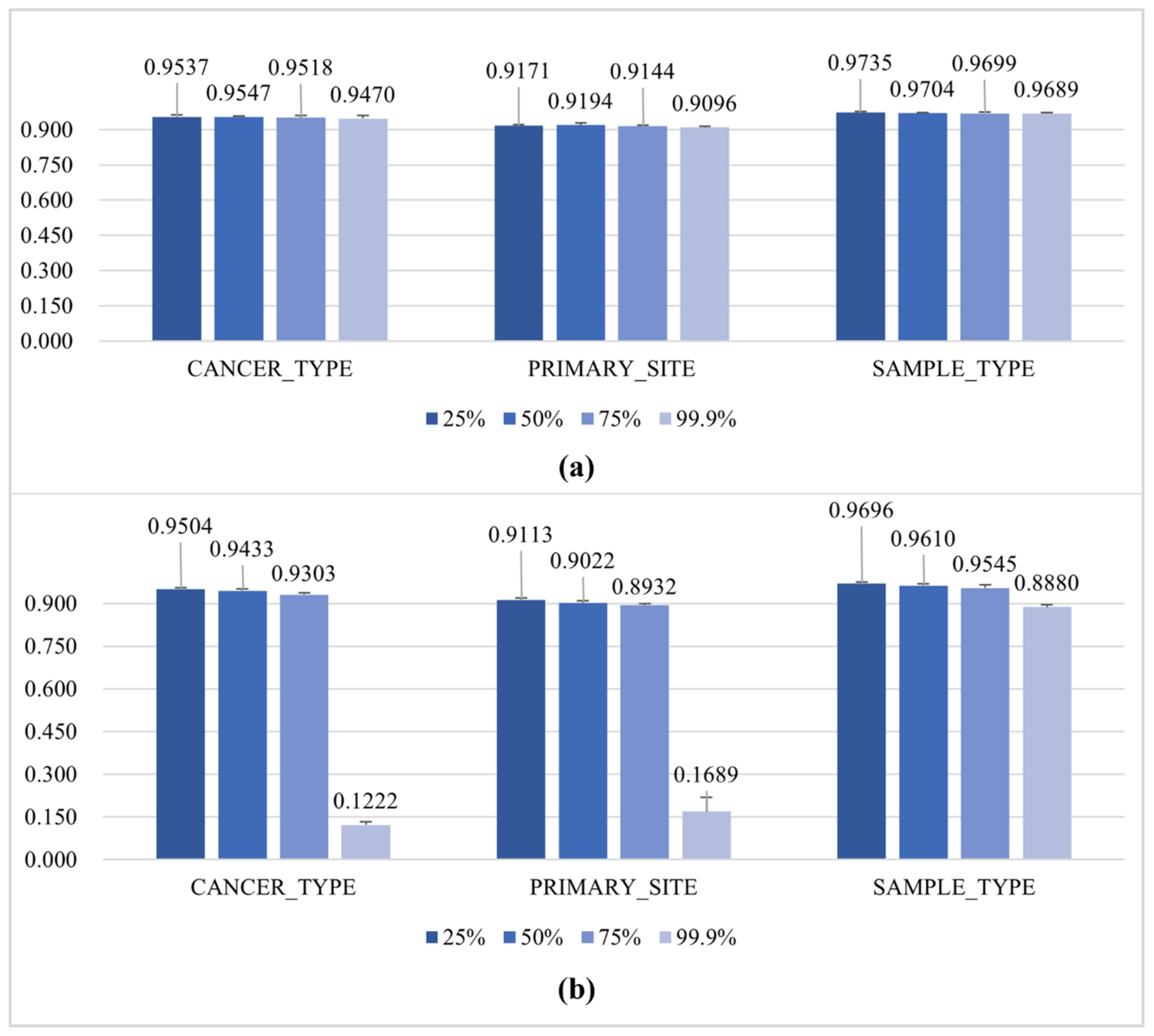
The performance of the proposed model in classifying cancer phenotype data was evaluated through three approaches. First, the classification performance for cancer phenotype was evaluated by comparing (1) a model trained with complete and incomplete data (“OUR”), (2) a model trained with only complete data (“111”), (3) a model that learned only mRNA gene expression and mRNA isoform expression data (“110”), and (4) a model that learned only DNA methylation data (“001”) (Figure 3). Second, we trained the “OUR+” model by adding a new omics type (miRNA expression) and evaluated its performance compared to the original “OUR” model. Third, the cancer phenotype classification performance according to the ratio of incomplete data in the learning data was compared between the “OUR” model and the “111” model (Figure 4).
The train–test data split for the K-fold cross-validation of the classification performance for cancer phenotypes was identical to the train–test data split for model learning. We established folds based on stratified sampling. Stratified sampling involves dividing the population into classes and randomly selecting n samples from each class. Purely random sampling methods can lead to biases, particularly when the data size is insufficient. Therefore, we divided the entire dataset into class-based groups and set the folds to be sampled in proportion to the counts of each class within the entire dataset. This ensured that even when the data were partitioned, the same distribution as the entire dataset was maintained, aiming to preserve the generalization of model learning. Among the 8773 samples with complete omics data, 20% of the samples (n = 1754) were used as the test dataset, and the remaining were used as the training dataset. Through this process, we generated five train–test datasets for K-fold cross-validation (K = 5) without overlapping data. For the phenotype data, “cancer type” included 33 classes, “primary site” included 32 classes, and “sample type” included 6 classes.
The baseline performance was that of the model expressed as “111”, which only learned complete data with all omics data. In comparison, the “OUR” model was a model that had additionally learned incomplete data and was trained on mRNA gene expression, mRNA isoform expression, and DNA methylation data. The “110” model refers to a model that learned from mRNA gene expression and mRNA isoform expression data, while “001” refers to a model that learned from DNA methylation data. These data groupings represent the types of omics groups in TCGA and SBIC. “OUR+” refers to a model that additionally learned miRNA mature strand expression data with the other three types of omics data.

3.2. Virtual Omics Generation Task

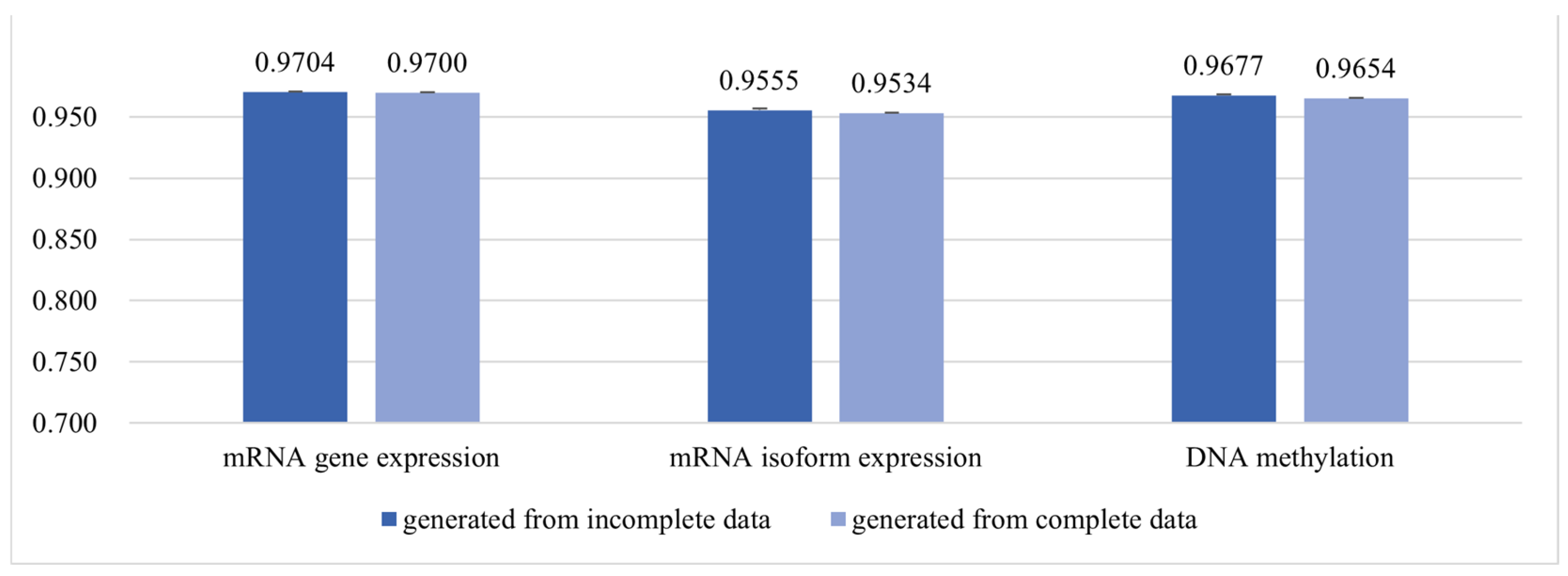
Three analyses were conducted to evaluate the quality of the virtual omics data generated by the proposed model. First, two experiments were conducted to validate the similarity between real and virtual omics data. One compared the data generation performance of the model using only complete data with the model using incomplete data using the “111” model and the “OUR” model (Figure 5). The other experiment focused on whether high-quality virtual omics data could be generated for non-existent omics data (Figure 6). Both experiments were conducted on five folds (1754 samples) divided using the stratified sampling technique. Virtual omics data were generated for all omics types for each sample and used to compute cosine similarity with the actual data. The average cosine similarity between the 1754 generated samples and the actual samples was calculated for each fold, and the values shown in the figures represent the mean and standard deviation of the cosine similarity averages for each fold.
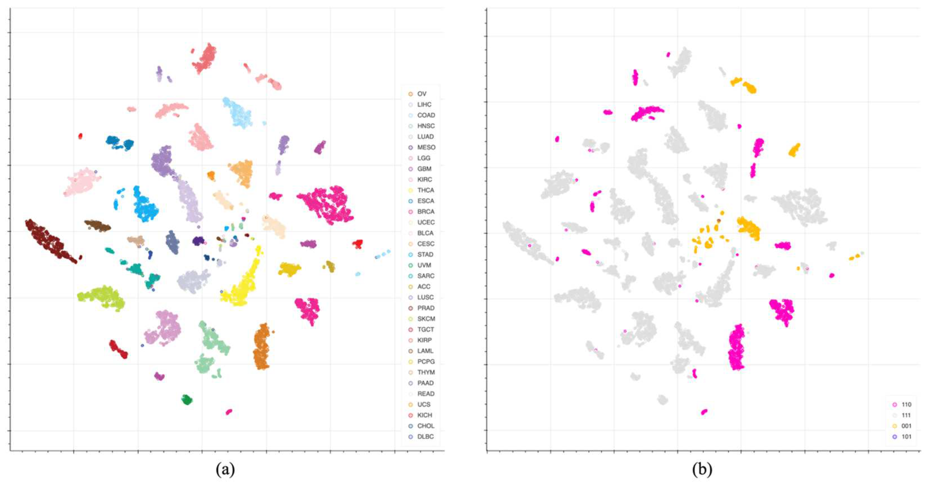
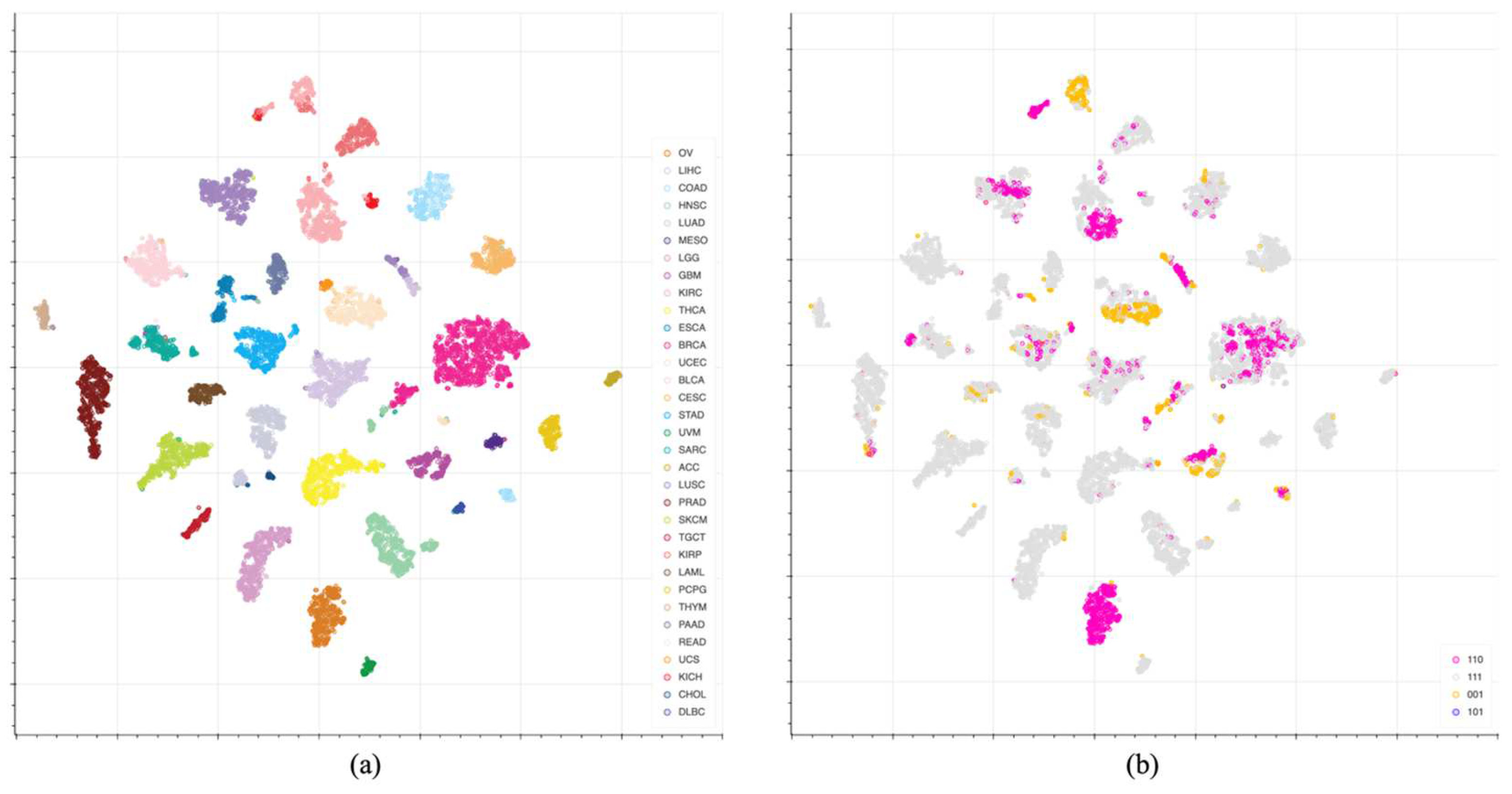
Second, through t-SNE visualization, clustering per class was calculated for individual phenotypes, and the effect of padding on cluster formation was determined (Figure 7 and Figures S4–S17). Third, for data replaced with padding data in the model learning (n = 1034 for mRNA gene expression, n = 1035 for mRNA isoform expression, and n = 1973 for DNA methylation), the virtual omics data were applied as substitutes. The proposed model, after learning, was used in the embedding of samples containing the virtual omics data and visualized via t-SNE to the clustering per class on individual phenotype data and the effect of reconstruction data on cluster formation (Figure 8, Figures S18 and S19). Finally, the actual omics data and virtual omics data were visualized via t-SNE to compare the distribution within the latent space (Figure 9 and Figures S20–S29).
The data used for the two experiments were identical to the K-fold cross-validation data for the phenotype classification task. Virtual omics data were generated through the model learned for each fold, and cosine similarity was calculated by comparing it with real omics data. The bar graphs in Figure 5 and Figure 6 present the average of five cosine similarity calculations.

4. Discussion

Embedding techniques typically extract task-dependent significant relationships in high-dimensional feature spaces and use them in downstream analysis. Many previous studies have relied on independent embedding techniques [34,35,36,37]; however, they included fewer samples for biomedical classification and prediction tasks. To address these issues, we investigated the rationale of embedding by adding virtual omics data, which resemble actual omics data.
In this study, the utility of the newly developed method over conventional methods that disallow the use of incomplete data was validated. Furthermore, virtual omics data that resemble actual omics data based on inferences on missing omics data were generated by two tasks: phenotype classification and virtual omics generation, using embedding data. In the phenotype classification task, a performance comparison experiment was conducted between the existing multi-omics model, which can learn only complete data, and the proposed model, which can also learn incomplete data. The average performance of the model was measured via K-fold cross-validation (K = 5). Performance comparison was performed on the “111” model trained on complete data only, the “OUR” model trained on incomplete data as well, and the “110” and “001” models trained on partial omics data only. As a result, the “OUR” model, trained with incomplete data, had the highest average performance in each phenotype (“OUR” cancer type: 0.9549, primary site: 0.9212, sample type: 0.9712) (Figure 3). Additionally, we compared the performance after training the proposed model using additional omics data. The proposed model was trained on three omics datasets (mRNA gene expression, mRNA isoform expression, and DNA methylation), while the additional training model was trained on four omics datasets (mRNA gene expression, mRNA isoform expression, DNA methylation, and miRNA mature strand expression). The average performance of the models was measured through K-fold cross-validation (K = 5). There was no significant performance difference between the two models (“OUR” cancer type: 0.9549, primary site: 0.9212, sample type: 0.9712; “OUR+” cancer type: 0.9586, primary site: 0.9175, sample type: 0.9717).
In terms of performance improvement, the proposed model did not show any significant improvement compared to the baseline model (a model that only trains on complete data). However, notably, our proposed model could learn robustly even in the absence of complete data. To demonstrate this, we conducted performance comparison experiments for extreme conditions for which complete data are rarely available. Figure 4 shows that the proposed model could maintain classification performance, whereas the conventional model that can learn only complete data exhibited a sharp performance drop in the relative absence of complete data in the training data (99.90%). Herein, “99.90%” is the dataset in which 99.9% of the complete data in the training data were replaced with incomplete data. Therefore, the number of complete data in the training data was low (only 3), preventing the existing model from properly training. Conversely, by introducing a padding strategy, the proposed model could proceed with learning that could produce meaningful results even in extreme situations lacking complete data.
Figure 5 shows the results of the measurement of the average similarity between the virtual omics data and the actual omics data generated through the baseline model (“111”), which learned on only complete data, and the proposed model (“OUR”), which also learned on incomplete data. For the three actual omics data types, the proposed model generated virtual omics data with a higher similarity than the data for the baseline model (baseline model—mRNA gene expression: 0.9436, mRNA isoform expression: 0.9387, DNA methylation: 0.9653; proposed model—mRNA gene expression: 0.9699, mRNA isoform expression: 0.9533, DNA methylation: 0.9656).
The proposed model is characterized by its ability to generate high-quality virtual omics data for missing omics data. This function cannot be performed in the basic model structure. Figure 6 depicts these characteristics. Incomplete data (“011”, “101”, and “110”) generated by removing specific omics data from complete data (“111”) were set as the input data of the model. Measuring the similarity between the actual omics data and virtual omics data generated from incomplete data revealed a high average cosine similarity of the three omics data types of 0.9646 (mRNA gene expression: 0.9704, mRNA isoform expression: 0.9555, DNA methylation: 0.9677).
Next, we performed visualizations to understand whether the proposed model can efficiently integrate different omics data sources by maintaining complementarity across omics data types and reducing the noise of partially independent features. Through t-SNE, we visualized the formation of clusters for three phenotypes (cancer type, primary site, and sample type) (Figure 7, Figures S4 and S5). Here, we captured the formation of multiple clusters of specific cancer types, such as BRCA, UCEC, KIRC, and STAD (Figure 7). This can be explained as distortion due to the formation of separate clusters depending on the presence or absence of padding data. To solve this distortion, we validated the effectiveness of virtual omics data in the virtual omics creation task. To this end, we replaced the padding with virtual omics data generated by model training and retrained the model. The embeddings generated from the retrained model were dimensionally reduced with t-SNE, and the formation of clusters for three phenotypes (cancer type, primary site, and sample type) was visualized. Similar to the previous case, the embedding data confirmed cluster formation for the three phenotypes (Figure 8, Figures S18 and S19). Additionally, compared to the previous visualization (Figure 7), certain data (e.g., BRCA, UCEC, KIRC, and STAD) that formed multiple clusters for the same carcinoma converged, indicating that the cluster distortion had been resolved (Figure 8).
Finally, we determined whether the virtual omics data generated by the proposed model differed from the actual omics data in the distribution within the latent space. To this end, the integration of actual and virtual data for a single-omics data type was visualized via t-SNE, and the difference in the distribution within the latent space was compared. Based on the cancer type, the virtual omics data formed similar clusters to those for the actual omics data in the latent space (Figure 9).
In summary, the novel approach developed in this study maximizes the use of multi-omics. For samples with incomplete omics data, learning outcomes from certain omics data were integrated with the learning data from samples with complete information, and the consequent embedding exhibited high quality and flexibility. Furthermore, the embedding led to the generation of virtual omics data that resembled actual omics data.
This study has certain limitations. First, our strategies were only developed and validated for a limited number of tasks, including cancer phenotype prediction, primary site prediction, and sample type prediction. However, with additional development, the strategy can be easily improved to include other classification and prediction tasks, such as target identification, identification of tissue origin and specific gene expression signatures, and multimodal predictions. In addition, other experimental data types, such as single-cell RNA-seq and competing endogenous RNA regulation, can eventually be included. However, as evident from the comparison experiment of training with additional omics data, simply adding data is insufficient to precisely analyze the relationships between omics data types and to enhance the performance. Second, the choice of primary site labeling (32 classes over 100 labels) should be investigated since it could be challenging in a single sample for a primary site. However, this was not the focus of this study. In future studies, advanced techniques such as attention mechanisms and graph neural networks can be utilized to comprehensively analyze the relationships between patients or omics, thus allowing weighted contributions from each data type to be reflected by global virtual omics data.

5. Conclusions

A model was developed with the embedding of SARC data for the Korean population from the SBIC (toward the construction of a national registry for rare cancers). However, owing to the inadequate number of samples in the Korean SBIC for learning by an AI model, publicly available cancer-related data in TCGA, including various genomic data types (from transcriptomes to epigenomes), were used. The SBIC data of the KBN (Korea Biobank Network) contain more limited data types, such as mRNA gene expression data and mRNA isoform expression data.
For an AI model, previous research has established that multi-omics data, compared to single-omics data, can more accurately capture the genetic features of cancer. Nevertheless, multi-omics data are often incomplete, limiting AI model application. For instance, the Korean SBIC data are incomplete; therefore, only partial omics data from TCGA could be used. Considering the vast array of genetic data related to cancer, using only parts of large-scale open databases in cases of incomplete data is a major limitation.
The newly proposed approach maximizes the utility of incomplete data. After integrating PanCan and SBIC data, values for mRNA gene expression, mRNA isoform expression, and DNA methylation were used as the input data. Samples that were missing omics data were treated by padding. While it sets the data specification for the learning by AI models, the padding strategy does not affect the learning process. For instance, when a given sample lacks DNA methylation data, the padding is not included in calculating the reconstruction loss for DNA methylation. In a series of steps, a model for embedding with high expandability to allow the maximized use of omics data was designed, and the generated embedding exhibited high quality and flexibility.
We validated that our proposed learning strategy maintains high classification performance and responds robustly to data sparsity to address the issues associated with incomplete omics data. The results of this study are expected to prove valuable for broad omics research. The novel methodology is also expected to be applicable across all AI-based domains.
However, the VAE architecture used in our study may struggle to capture key features within complex or high-dimensional distributions, such as omics data. This difficulty arises because assuming a simple distribution, such as a Gaussian distribution in the latent space, may not adequately reflect the complexity of the data distribution. Additionally, the latent space learned through the VAE may be intricately entangled, which can complicate interpreting the model’s data generation and prediction processes.
To address these issues, we plan to design a model that can better capture the complexity of data distributions by utilizing a transformer-based VAE architecture. Furthermore, we intend to incorporate a process that allows researchers to understand and interpret the model’s outputs by visualizing the data generation and cancer phenotype prediction processes through attention visualization.
Supplementary Materials

The following supporting information can be downloaded at: https://www.mdpi.com/article/10.3390/ai5030078/s1, Figure S1: Histogram visualization and statistics of the total mRNA gene expression; Figure S2: Histogram visualization and statistics of the total mRNA isoform expression; Figure S3: Histogram visualization and statistics of the total DNA methylation; Figure S4: t-SNE visualization of the embedded data for the proposed model after dimensionality reduction; Figure S5: t-SNE visualization of the embedded data for the proposed model after dimensionality reduction; Figure S6: t-SNE visualization of the mRNA gene expression data for the proposed model after dimensionality reduction; Figure S7: t-SNE visualization of the mRNA gene expression data for the proposed model after dimensionality reduction; Figure S8: t-SNE visualization of the mRNA gene expression data for the proposed model after dimensionality reduction; Figure S9: t-SNE visualization of the mRNA gene expression data for the proposed model after dimensionality reduction; Figure S10: t-SNE visualization of the mRNA isoform expression data for the proposed model after dimensionality reduction; Figure S11: t-SNE visualization of the mRNA isoform expression data for the proposed model after dimensionality reduction; Figure S12: t-SNE visualization of the mRNA isoform expression data for the proposed model after dimensionality reduction; Figure S13: t-SNE visualization of the mRNA isoform expression data for the proposed model after dimensionality reduction; Figure S14: t-SNE visualization of the DNA methylation data for the proposed model after dimensionality reduction; Figure S15: t-SNE visualization of the DNA methylation data for the proposed model after dimensionality reduction; Figure S16: t-SNE visualization of the DNA methylation data for the proposed model after dimensionality reduction; Figure S17: t-SNE visualization of the DNA methylation data for the proposed model after dimensionality reduction; Figure S18: t-SNE visualization of the embedding data for the proposed model with learning from virtual omics data as an alternative to padding; Figure S19: t-SNE visualization of the embedding data for the proposed model with learning from virtual omics data as an alternative to padding; Figure S20: t-SNE visualization of the mRNA gene expression data for the proposed model with learning from virtual omics data as an alternative to padding; Figure S21: t-SNE visualization of the mRNA gene expression data for the proposed model with learning from virtual omics data as an alternative to padding; Figure S22: t-SNE visualization of the mRNA gene expression data for the proposed model with learning from virtual omics data as an alternative to padding; Figure S23: t-SNE visualization of the mRNA gene expression data for the proposed model with learning from virtual omics data as an alternative to padding; Figure S24: t-SNE visualization of the mRNA isoform expression data for the proposed model with learning from virtual omics data as an alternative to padding; Figure S25: t-SNE visualization of the mRNA isoform expression data for the proposed model with learning from virtual omics data as an alternative to padding; Figure S26: t-SNE visualization of the mRNA isoform expression data for the proposed model with learning from virtual omics data as an alternative to padding; Figure S27: t-SNE visualization of the mRNA isoform expression data for the proposed model with learning from virtual omics data as an alternative to padding; Figure S28: t-SNE visualization of the DNA methylation data for the proposed model with learning from virtual omics data as an alternative to padding; Figure S29: t-SNE visualization of the DNA methylation data for the proposed model with learning from virtual omics data as an alternative to padding.

Author Contributions

Conceptualization, H.-S.L. and S.-H.H.; methodology, H.-S.L.; formal analysis, G.-H.K., J.-H.J. and J.-W.A.; investigation, H.-S.L.; writing—original draft preparation, H.-S.L.; writing—review and editing, J.-H.K., H.-J.Y. and E.-Y.L. All authors have read and agreed to the published version of the manuscript.

Funding

This research was supported by the National Institute of Health (NIH) research project (project No. 2024-ER0511-00).

Institutional Review Board Statement

This study was conducted in accordance with the Declaration of Helsinki and approved by the Institutional Review Board of the National Cancer Center Korea (IRB number: NCC2021-0184, date of approval: 29 June 2021).

Informed Consent Statement

Informed consent was obtained from all subjects involved in this study.

Data Availability Statement

The data presented in this study are available in UCSC Xena at https://xena.ucsc.edu/, cohort TCGA Pan-Cancer (PANCAN). These data were derived from the following resources available in the public domain: https://xenabrowser.net/datapages/?cohort=TCGA%20Pan-Cancer%20(PANCAN)&removeHub=http%3A%2F%2F127.0.0.1%3A7222. Accessed on 1 August 2022. The data analyzed during the current study and the data included in Korea Biobank Network were generated from the Korea Disease Control and Prevention Agency for the Korea Biobank Project and are not publicly available but are available from the corresponding author on reasonable request.

Conflicts of Interest

Author Jaehwan Jeong and Author Jinwoo Ahn were employed by the company Celemics, Inc. The remaining authors declare that the research was conducted in the absence of any commercial or financial relationships that could be construed as a potential conflict of interest.

References

  1. Misra, B.B.; Langefeld, C.D.; Olivier, M.; Cox, L.A. Integrated omics: Tools, advances, and future approaches. J. Mol. Endocrinol. 2018, 62, R21–R45. [Google Scholar] [CrossRef]
  2. Zeeshan, S.; Xiong, R.; Liang, B.T.; Ahmed, Z. 100 years of evolving gene–disease complexities and scientific debutants. Brief Bioinform. 2020, 21, 885–905. [Google Scholar] [CrossRef]
  3. Yan, J.; Risacher, S.L.; Shen, L.; Saykin, A.J. Network approaches to systems biology analysis of complex disease: Integrative methods for multi-omics data. Brief Bioinform. 2018, 19, 1370–1381. [Google Scholar] [CrossRef]
  4. Son, J.W.; Shoaie, S.; Lee, S. Systems biology: A multi-omics integration approach to metabolism and the microbiome. Endocrinol. Metab. 2020, 35, 507–514. [Google Scholar] [CrossRef] [PubMed]
  5. Siegfried, Z.; Simon, I. DNA methylation and gene expression. Wiley Interdiscip. Rev. Syst. Biol. Med. 2010, 2, 362–371. [Google Scholar] [CrossRef] [PubMed]
  6. Manolio, T.A. Genomewide association studies and assessment of the risk of disease. N. Engl. J. Med. 2010, 363, 166–176. [Google Scholar] [CrossRef] [PubMed]
  7. Trapnell, C.; Roberts, A.; Goff, L.; Pertea, G.; Kim, D.; Kelley, D.R.; Pimentel, H.; Salzberg, S.L.; Rinn, J.L.; Pachter, L. Differential gene and transcript expression analysis of RNA-seq experiments with TopHat and Cufflinks. Nat. Protoc. 2012, 7, 562–578. [Google Scholar] [CrossRef]
  8. Lokk, K.; Modhukur, V.; Rajashekar, B.; Märtens, K.; Mägi, R.; Kolde, R.; Koltšina, M.; Nilsson, T.K.; Vilo, J.; Salumets, A.; et al. DNA methylome profiling of human tissues identifies global and tissue-specific methylation patterns. Genome Biol. 2014, 15, 3248. [Google Scholar] [CrossRef]
  9. Frantzi, M.; Latosinska, A.; Flühe, L.; Hupe, M.C.; Critselis, E.; Kramer, M.W.; Merseburger, A.S.; Mischak, H.; Vlahou, A. Developing proteomic biomarkers for bladder cancer: Towards clinical application. Nat. Rev. Urol. 2015, 12, 317–330. [Google Scholar] [CrossRef]
  10. Zhao, J.; Zhu, Y.; Hyun, N.; Zeng, D.; Uppal, K.; Tran, V.T.; Yu, T.; Jones, D.; He, J.; Lee, E.T.; et al. Novel metabolic markers for the risk of diabetes development in American Indians. Diabetes Care 2015, 38, 220–227. [Google Scholar] [CrossRef]
  11. Reel, P.S.; Reel, S.; Pearson, E.; Trucco, E.; Jefferson, E. Using machine learning approaches for multi-omics data analysis: A review. Biotechnol. Adv. 2021, 49, 107739. [Google Scholar] [CrossRef] [PubMed]
  12. Koppad, S.; Annappa, B.; Gkoutos, G.V.; Acharjee, A. Cloud computing enabled big multi-omics data analytics. Bioinform. Biol. Insights 2021, 15, 11779322211035921. [Google Scholar] [CrossRef] [PubMed]
  13. Subramanian, I.; Verma, S.; Kumar, S.; Jere, A.; Anamika, K. Multi-omics data integration, interpretation, and its application. Bioinform. Biol. Insights 2020, 14, 1177932219899051. [Google Scholar] [CrossRef] [PubMed]
  14. Sun, Y.V.; Hu, Y.J. Integrative analysis of multi-omics data for discovery and functional studies of complex human diseases. Adv. Genet. 2016, 93, 147–190. [Google Scholar]
  15. Bersanelli, M.; Mosca, E.; Remondini, D.; Giampieri, E.; Sala, C.; Castellani, G.; Milanesi, L. Methods for the integration of multi-omics data: Mathematical aspects. BMC Bioinform. 2016, 17, 15. [Google Scholar] [CrossRef]
  16. Meng, C.; Zeleznik, O.A.; Thallinger, G.G.; Kuster, B.; Gholami, A.M.; Culhane, A.C. Dimension reduction techniques for the integrative analysis of multi-omics data. Brief Bioinform. 2016, 17, 628–641. [Google Scholar] [CrossRef]
  17. Hasin, Y.; Seldin, M.; Lusis, A. Multi-omics approaches to disease. Genome Biol. 2017, 18, 83. [Google Scholar] [CrossRef]
  18. Lin, E.; Lane, H.Y. Machine learning and systems genomics approaches for multi-omics data. Biomark Res. 2017, 5, 2. [Google Scholar] [CrossRef] [PubMed]
  19. Huang, S.; Chaudhary, K.; Garmire, L.X. More is better: Recent progress in multi-omics data integration methods. Front. Genet. 2017, 8, 84. [Google Scholar] [CrossRef] [PubMed]
  20. Vasaikar, S.V.; Straub, P.; Wang, J.; Zhang, B. LinkedOmics: Analyzing multi-omics data within and across 32 cancer types. Nucleic Acids Res. 2018, 46, D956–D963. [Google Scholar] [CrossRef] [PubMed]
  21. Argelaguet, R.; Velten, B.; Arnol, D.; Dietrich, S.; Zenz, T.; Marioni, J.C.; Buettner, F.; Huber, W.; Stegle, O. Multi-omics factor analysis-a framework for unsupervised integration of multi-omics data sets. Mol. Syst. Biol. 2018, 14, e8124. [Google Scholar] [CrossRef]
  22. Lánczky, A.; Győrffy, B. Web-based survival analysis tool tailored for medical research (KmPlot): Development and implementation. J. Med. Internet Res. 2021, 23, e27633. [Google Scholar] [CrossRef]
  23. Picard, M.; Scott-Boyer, M.P.; Bodein, A.; Périn, O.; Droit, A. Integration strategies of multi-omics data for machine learning analysis. Comput. Struct. Biotechnol. J. 2021, 19, 3735–3746. [Google Scholar] [CrossRef]
  24. Mo, Q.; Wang, S.; Seshan, V.E.; Olshen, A.B.; Schultz, N.; Sander, C.; Powers, R.S.; Ladanyi, M.; Shen, R. Pattern discovery and cancer gene identification in integrated cancer genomic data. Proc. Natl. Acad. Sci. USA 2013, 110, 4245–4250. [Google Scholar] [CrossRef]
  25. Duan, R.; Gao, L.; Gao, Y.; Hu, Y.; Xu, H.; Huang, M.; Song, K.; Wang, H.; Dong, Y.; Jiang, C.; et al. Evaluation and comparison of multi-omics data integration methods for cancer subtyping. PLoS Comput. Biol. 2021, 17, e1009224. [Google Scholar] [CrossRef]
  26. Hung, A.J. Can machine-learning algorithms replace conventional statistics? BJU Int. 2019, 123, 1. [Google Scholar] [CrossRef]
  27. Barnett-Itzhaki, Z.; Elbaz, M.; Butterman, R.; Amar, D.; Amitay, M.; Racowsky, C.; Orvieto, R.; Hauser, R.; Baccarelli, A.A.; Machtinger, R. Machine learning vs. classic statistics for the prediction of IVF outcomes. J. Assist. Reprod. Genet. 2020, 37, 2405–2412. [Google Scholar] [CrossRef]
  28. Sammut, S.J.; Crispin-Ortuzar, M.; Chin, S.F.; Provenzano, E.; Bardwell, H.A.; Ma, W.; Cope, W.; Dariush, A.; Dawson, S.J.; Abraham, J.E.; et al. Multi-omic machine learning predictor of breast cancer therapy response. Nature 2022, 601, 623–629. [Google Scholar] [CrossRef]
  29. Garali, I.; Adanyeguh, I.M.; Ichou, F.; Perlbarg, V.; Seyer, A.; Colsch, B.; Moszer, I.; Guillemot, V.; Durr, A.; Mochel, F.; et al. A strategy for multimodal data integration: Application to biomarkers identification in spinocerebellar ataxia. Brief Bioinform. 2018, 19, 1356–1369. [Google Scholar] [CrossRef]
  30. Kavakiotis, I.; Tsave, O.; Salifoglou, A.; Maglaveras, N.; Vlahavas, I.; Chouvarda, I. Machine learning and data mining methods in diabetes research. Comput. Struct. Biotechnol. J. 2017, 15, 104–116. [Google Scholar] [CrossRef] [PubMed]
  31. Joshi, A.; Rienks, M.; Theofilatos, K.; Mayr, M. Systems biology in cardiovascular disease: A multiomics approach. Nat. Rev. Cardiol. 2021, 18, 313–330. [Google Scholar] [CrossRef] [PubMed]
  32. Frankish, A.; Diekhans, M.; Jungreis, I.; Lagarde, J.; Loveland, J.E.; Mudge, J.M.; Sisu, C.; Wright, J.C.; Armstrong, J.; Barnes, I.; et al. GENCODE 2021. Nucleic Acids Res. 2021, 49, D916–D923. [Google Scholar] [CrossRef]
  33. Wang, Z.; Wu, X.; Wang, Y. A framework for analyzing DNA methylation data from Illumina Infinium HumanMethylation450 BeadChip. BMC Bioinform. 2018, 19, 115. [Google Scholar] [CrossRef]
  34. Engreitz, J.M.; Daigle, B.J., Jr.; Marshall, J.J.; Altman, R.B. Independent component analysis: Mining microarray data for fundamental human gene expression modules. J. Biomed. Inform. 2010, 43, 932–944. [Google Scholar] [CrossRef] [PubMed]
  35. Yang, Z.; Michailidis, G. A non-negative matrix factorization method for detecting modules in heterogeneous omics multi-modal data. Bioinformatics 2016, 32, 1–8. [Google Scholar] [CrossRef] [PubMed]
  36. Shen-Orr, S.S.; Gaujoux, R. Computational deconvolution: Extracting cell type-specific information from heterogeneous samples. Curr. Opin. Immunol. 2013, 25, 571–578. [Google Scholar] [CrossRef]
  37. Way, G.P.; Greene, C.S. Extracting a biologically relevant latent space from cancer transcriptomes with variational autoencoders. Biocomputing 2018, 23, 80–91. [Google Scholar]
  38. Kingma, D.P.; Welling, M. Auto-encoding variational bayes. arXiv 2014, arXiv:1312.6114. [Google Scholar] [CrossRef]
  39. Gomez-Cabrero, D.; Abugessaisa, I.; Maier, D.; Teschendorff, A.; Merkenschlager, M.; Gisel, A.; Ballestar, E.; Bongcam-Rudloff, E.; Conesa, A.; Tegnér, J. Data integration in the era of omics: Current and future challenges. BMC Syst. Biol. 2014, 8, I1. [Google Scholar] [CrossRef]
  40. Cancer Genome Atlas Research Network; Weinstein, J.N.; Collisson, E.A.; Mills, G.B.; Shaw, K.R.; Ozenberger, B.A.; Ellrott, K.; Shmulevich, I.; Sander, C.; Stuart, J.M. The Cancer Genome Atlas Pan-Cancer analysis project. Nat. Genet. 2013, 45, 1113–1120. [Google Scholar] [CrossRef]
  41. Chiu, Y.C.; Chen, H.H.; Zhang, T.; Zhang, S.; Gorthi, A.; Wang, L.J.; Huang, Y.; Chen, Y. Predicting drug response of tumors from integrated genomic profiles by deep neural networks. BMC Med. Genom. 2019, 12, 18. [Google Scholar]
  42. Cao, Z.J.; Gao, G. Multi-omics single-cell data integration and regulatory inference with graph-linked embedding. Nat. Biotechnol. 2022, 40, 1458–1466. [Google Scholar] [CrossRef] [PubMed]
  43. Du, J.H.; Cai, Z.; Roeder, K. Robust probabilistic modeling for single-cell multimodal mosaic integration and imputation via scVAEIT. Proc. Natl. Acad. Sci. USA. 2022, 119, e2214414119. [Google Scholar] [CrossRef] [PubMed]
  44. Goldman, M.J.; Craft, B.; Hastie, M.; Repečka, K.; McDade, F.; Kamath, A.; Banerjee, A.; Luo, Y.; Rogers, D.; Brooks, A.N.; et al. Visualizing and interpreting cancer genomics data via the Xena platform. Nat. Biotechnol. 2020, 38, 675–678. [Google Scholar] [CrossRef] [PubMed]
  45. Barrier, A.; Lemoine, A.; Boelle, P.Y.; Tse, C.; Brault, D.; Chiappini, F.; Breittschneider, J.; Lacaine, F.; Houry, S.; Huguier, M.; et al. Colon cancer prognosis prediction by gene expression profiling. Oncogene 2005, 24, 6155–6164. [Google Scholar] [CrossRef]
  46. Vitting-Seerup, K.; Sandelin, A. The landscape of isoform switches in human cancers. Mol. Cancer Res. 2017, 15, 1206–1220. [Google Scholar] [CrossRef]
  47. Yang, I.S.; Son, H.; Kim, S.; Kim, S. ISOexpresso: A web-based platform for isoform-level expression analysis in human cancer. BMC Genom. 2016, 17, 631. [Google Scholar] [CrossRef]
  48. Locke, W.J.; Guanzon, D.; Ma, C.; Liew, Y.J.; Duesing, K.R.; Fung, K.Y.C.; Ross, J.P. DNA methylation cancer biomarkers: Translation to the clinic. Front. Genet. 2019, 10, 1150. [Google Scholar] [CrossRef]
  49. Lightning PT. Available online: https://www.pytorchlightning.ai/ (accessed on 8 November 2022).
  50. PyTorch. Available online: https://pytorch.org/ (accessed on 8 November 2022).
  51. Tan, O.; Liu, L.; You, Q.; Wang, J.; Chen, A.; Ing, E.; Morrison, J.C.; Jia, Y.; Huang, D. Focal loss analysis of nerve fiber layer reflectance for glaucoma diagnosis. Transl. Vis. Sci. Technol. 2021, 10, 9. [Google Scholar] [CrossRef]
  52. Scikit-Learn. Available online: https://scikit-learn.org/stable/ (accessed on 8 November 2022).
  53. Bokeh. Available online: https://docs.bokeh.org/en/latest/ (accessed on 8 November 2022).
Figure 1. Schematic comparing complete and incomplete data. Complete data are data in which all omics data to be utilized exist, and incomplete data are data in which some of the omics data to be utilized are missing.
Ai 05 00078 g001
Figure 2. Structure of the proposed model. Each layer of the model is composed of linear neural networks with the rectified linear unit activation function and layer normalization. In the absence of specific omics data for a given sample, the input is 0. The output of the encoder for each omics data type is concatenated as a single vector and transferred to the layer that generates the final encoding vector. The output of the layer generating the final encoding vector is transferred to the mean and standard deviation layer to realize the reparameterization of the VAE. A latent vector is generated based on the output of the mean and standard deviation layer and serves as the input for the expanded classification model that infers cancer phenotypes for each decoder.
Ai 05 00078 g002
Figure 3. Comparison of phenotype classification performance (weighted F1 score). Cross-validated average performance of the classification model for cancer phenotype based on omics and embedding data. The classification of phenotypes was performed via in-model classifiers.
Ai 05 00078 g003
Figure 4. Comparison of phenotype classification performance according to the data sparsity ratio (weighted F1 score) (i.e., sparsity of complete data). Classification of phenotypes was performed via in-model classifiers. (a) Data sparsity experiment result for the “OUR” model, which can train complete and incomplete data; (b) data sparsity experiment result for the “111” model, which can only learn complete data. The values 25, 50, 75, and 99.9 are the percentages of complete data converted to incomplete data in the training dataset. Conversion is achieved by randomly removing some of the omics data. Higher numbers increase the sparsity of complete data in the training dataset, and the amount of training data can vary depending on the model’s structure. For example, “25%” of (a) is the training result of the “OUR” model trained on data, with 25% of the complete data in the training dataset transformed into incomplete data. Since the “OUR” model can be trained on both complete and incomplete data, even if complete data are converted to incomplete data, the amount of training data does not decrease. In contrast, the “111” model can only learn complete data. Therefore, “25%” in (b) shows the result of learning the reduced training data, with 25% of the complete data converted to incomplete data.
Ai 05 00078 g004
Figure 5. Comparison of the calculated cosine similarity between the virtual data and original data. The dataset used for testing comprised complete data only. The closer the cosine similarity is to 1, the more similar the virtual omics data were to the original.
Ai 05 00078 g005
Figure 6. Comparison of the calculated cosine similarity between the virtual data and original data. The dataset used for testing was divided into three parts, comprising data (“011”, “101”, and “110”) with all specific omics data omitted from the complete data (“111”). The same “OUR” model was used for the three datasets. Performance was measured by generating virtual omics data for omitted data in each dataset and then measuring cosine similarity with real omics data. For example, “011”, which is data that deliberately exclude mRNA gene expression from the complete data, is used to measure performance on mRNA gene expression; “011” creates a latent vector from those data and uses them as inputs to a decoder that reconstructs the mRNA gene expression data. Through this process, mRNA gene expression data that do not exist in the input data can be virtually generated. The closer the cosine similarity is to 1, the more similar the virtual omics data were to the original.
Ai 05 00078 g006
Figure 7. t-SNE visualization of the embedding data for the proposed model after dimensionality reduction. The colors and abbreviations indicate cancer types (a) and the type of omics data (b). ACC: adrenocortical carcinoma; BLCA: bladder urothelial carcinoma; BRCA: breast invasive carcinoma; CESC: cervical squamous cell carcinoma and endocervical adenocarcinoma; CHOL: cholangiocarcinoma; COAD: colon adenocarcinoma; DLBC: diffuse large B-cell lymphoma; ESCA: esophageal carcinoma; GBM: glioblastoma multiforme; HNSC: head and neck squamous cell carcinoma; KICH: kidney chromophobe; KIRC: kidney renal clear cell carcinoma; KIRP: kidney renal papillary cell carcinoma; LAML: acute myeloid leukemia; LGG: brain lower grade glioma; LIHC: liver hepatocellular carcinoma; LUAD: lung adenocarcinoma; LUSC: lung squamous cell carcinoma; MESO: mesothelioma; OV: ovarian serous cystadenocarcinoma; PAAD: pancreatic adenocarcinoma; PCPG: pheochromocytoma and paraganglioma; PRAD: prostate adenocarcinoma; READ: rectum adenocarcinoma; SARC: sarcoma; SKCM: skin cutaneous melanoma; STAD: stomach adenocarcinoma; TGCT: testicular germ cell tumors; THCA: thyroid carcinoma; THYM: thymoma; UCEC: uterine corpus endometrial carcinoma; UCS: uterine carcinosarcoma; UVM: uveal melanoma. 001: DNA methylation data exist, but mRNA gene expression and mRNA isoform expression data do not exist; 101: mRNA gene expression and DNA methylation data exist, but mRNA isoform expression data do not exist; 110: mRNA gene expression and mRNA isoform expression data exist, but DNA methylation data do not exist; 111: mRNA gene expression, mRNA isoform expression and DNA methylation data exist.
Ai 05 00078 g007
Figure 8. t-SNE visualization of the embedding data for the proposed model with learning from virtual omics data as an alternative to padding. The colors and abbreviations indicate cancer types (a) and the type of omics data (b). ACC: adrenocortical carcinoma; BLCA: bladder urothelial carcinoma; BRCA: breast invasive carcinoma; CESC: cervical squamous cell carcinoma and endocervical adenocarcinoma; CHOL: cholangiocarcinoma; COAD: colon adenocarcinoma; DLBC: diffuse large B-cell lymphoma; ESCA: esophageal carcinoma; GBM: glioblastoma multiforme; HNSC: head and neck squamous cell carcinoma; KICH: kidney chromophobe; KIRC: kidney renal clear cell carcinoma; KIRP: kidney renal papillary cell carcinoma; LAML: acute myeloid leukemia; LGG: brain lower grade glioma; LIHC: liver hepatocellular carcinoma; LUAD: lung adenocarcinoma; LUSC: lung squamous cell carcinoma; MESO: mesothelioma; OV: ovarian serous cystadenocarcinoma; PAAD: pancreatic adenocarcinoma; PCPG: pheochromocytoma and paraganglioma; PRAD: prostate adenocarcinoma; READ: rectum adenocarcinoma; SARC: sarcoma; SKCM: skin cutaneous melanoma; STAD: stomach adenocarcinoma; TGCT: testicular germ cell tumors; THCA: thyroid carcinoma; THYM: thymoma; UCEC: uterine corpus endometrial carcinoma; UCS: uterine carcinosarcoma; UVM: uveal melanoma. 001: DNA methylation data exist, but mRNA gene expression and mRNA isoform expression data do not exist; 101: mRNA gene expression and DNA methylation data exist, but mRNA isoform expression data do not exist; 110: mRNA gene expression and mRNA isoform expression data exist, but DNA methylation data do not exist; 111: mRNA gene expression, mRNA isoform expression and DNA methylation data exist.
Ai 05 00078 g008
Figure 9. t-SNE visualization of the DNA methylation data after dimensionality reduction for the actual and virtual data. The colors and abbreviations indicate cancer types (a) and the type of omics data (b). ACC: adrenocortical carcinoma; BLCA: bladder urothelial carcinoma; BRCA: breast invasive carcinoma; CESC: cervical squamous cell carcinoma and endocervical adenocarcinoma; CHOL: cholangiocarcinoma; COAD: colon adenocarcinoma; DLBC: diffuse large B-cell lymphoma; ESCA: esophageal carcinoma; GBM: glioblastoma multiforme; HNSC: head and neck squamous cell carcinoma; KICH: kidney chromophobe; KIRC: kidney renal clear cell carcinoma; KIRP: kidney renal papillary cell carcinoma; LAML: acute myeloid leukemia; LGG: brain lower grade glioma; LIHC: liver hepatocellular carcinoma; LUAD: lung adenocarcinoma; LUSC: lung squamous cell carcinoma; MESO: mesothelioma; OV: ovarian serous cystadenocarcinoma; PAAD: pancreatic adenocarcinoma; PCPG: pheochromocytoma and paraganglioma; PRAD: prostate adenocarcinoma; READ: rectum adenocarcinoma; SARC: sarcoma; SKCM: skin cutaneous melanoma; STAD: stomach adenocarcinoma; TGCT: testicular germ cell tumors; THCA: thyroid carcinoma; THYM: thymoma; UCEC: uterine corpus endometrial carcinoma; UCS: uterine carcinosarcoma; UVM: uveal melanoma. 001: DNA methylation data exist, but mRNA gene expression and mRNA isoform expression data do not exist; 101: mRNA gene expression and DNA methylation data exist, but mRNA isoform expression data do not exist; 110: mRNA gene expression and mRNA isoform expression data exist, but DNA methylation data do not exist; 111: mRNA gene expression, mRNA isoform expression and DNA methylation data exist.
Ai 05 00078 g009
Table 1. Omics data type and quantity according to availability.
Data TypemRNA
Gene Expression
mRNA
Isoform Expression
DNA
Methylation
Data
Quantity
Type 1 (111)1118773
Type 2 (110)1101767
Type 3 (001)001828
Type 4 (101)1011
0: omics data do not exist, 1: omics data are present.
Table 2. The search range and optimized values of hyperparameters.
HyperparametersSearch RangeOptimized Value
Epochs[30–500]500
Batch size[8–512]32
Latent dimension[100–500]100
Learning rate[0.0001–0.001]0.0005
KL coefficient[0.0001–0.0005]0.00025
Clip norm[10.0–100.0]50.0
Optimizer[Adam, AdamW, Adabelief]Adabelief
Seed-42
Disclaimer/Publisher’s Note: The statements, opinions and data contained in all publications are solely those of the individual author(s) and contributor(s) and not of MDPI and/or the editor(s). MDPI and/or the editor(s) disclaim responsibility for any injury to people or property resulting from any ideas, methods, instructions or products referred to in the content.