Applications of Gaussian Boson Sampling to Solve Some Chemistry Problems

Abstract

Quantum computers, due to their superposition and entanglement properties, provide significant advantages in solving certain problems compared with classical computers. Therefore, it is crucial to identify issues that can be efficiently solved by noisy intermediate-scale quantum (NISQ) systems. Xanadu has introduced the X8 quantum chip, based on integrated photonic technology, along with important photonic platforms such as Strawberry Fields and Gaussian Boson Sampling (GBS), to solve specific computational problems. In this review article, after reviewing Boson Sampling (BS) and Gaussian Boson Sampling (GBS), we discuss the relationship between GBS and graph theory, including how graphs can be encoded in GBS. Some applications of GBS, particularly molecular docking and molecular vibrations, are also considered. The future goal of this study is to identify problems that can be represented as small graphs and solved using GBS with a limited number of optical modes.

1. Introduction

Classical computers, which have played an important role in scientific progress, were developed in the 1950s. They are digital machines that use transistors to store data as binary data in individual bits, 0 and 1. In contrast, quantum computers use quantum mechanical properties such as superposition and entanglement to generate states that scale with the number of quantum bits (qubits). The capability of a quantum device to stay in multiple states at the same time is called superposition, and the robust correlation between quantum particles is known as entanglement. These phenomena cause a qubit in the quantum computer to represent 1 and 0 at the same time as a result of the superposition of 0 and 1. In other words, a qubit can be 0, 1, or both 0 and 1 at the same time, with a numerical constant demonstrating the probability for each state. This property of a qubit allows quantum computers to show improvement in solving multipart problems that recent classical computers cannot perform or take a long time to achieve the best results [1,2,3].

The quantum computing idea, which combines the concepts of mathematics, physics, computer science, and engineering, was first proposed in 1980 by Yuri Manin, a Russian mathematician [4,5,6,7]. In 1982, Richard Feynman [8] announced the conception of the quantum computer and said “Nature isn’t classical, and when you need to simulate nature, you’d better make it quantum mechanical” [9]. Classical computers face fundamental limitations when simulating quantum systems, as the computational resources required generally grow exponentially with the system size. This challenge is well recognized in quantum complexity theory and motivates the use of quantum-based computational methods [7,8,10,11]. Quantum computers, because of their quantum mechanical properties, can simulate quantum systems effectively and provide exponential improvements compared with classical computing for specific computational problems [9,12,13,14]. Quantum computing has had noteworthy developments in recent years from a community of quantum chemistry, physics, and information theory specialists, especially through the advances of Shor’s algorithm [15]. Quantum computing is divided into two key methods: analog quantum computing and gate-based quantum computing. The first operates by producing a primary set of qubits demonstrating all probable solutions to a task and applying the properties of superposition and entanglement to identify an optimal solution. Among analog quantum computing methods, such as quantum simulation, quantum annealing, and adiabatic quantum computing, a quantum annealing machine is the complete kind of analog quantum computer that can resolve certain optimization problems, for instance, optimizing drug design [16,17,18], traffic, and transportation, without carrying out computations on single qubits. Gate-based quantum computing breaks down a problem into a sequence of gates or basic operations like the building blocks of a classical computer or logic gates, which carry out operations on bits [19].

Studies in gate-based quantum computing have usually concentrated on two systems: noisy intermediate-scale quantum (NISQ) computers [20] and future fault-tolerant quantum computers (FTQCs) [21]. Some applications of quantum computing, such as identifying the prime elements of a composite number [15,22] and Hamiltonian simulation [23,24], need universal fault-tolerant quantum computers (FTQCs) [21], which, because of the experimental challenges of constructing FTQCs, are not expected to be accessible soon [6,13,25,26]. As a substitute, NISQ systems, which have a few physical qubits and imperfect operations and a limited size, connectivity, and circuit depth [20], are accessible at present. NISQ systems, due to their weaker hardware compared with universal quantum computers, limited computational resources, and lack of error correction [19,20,27], can only be used to perform specific problems [28,29,30]. So, the specification of problems that could be solved with NISQ systems is very important [6,25,27].

Quantum computers can be classified based on two types of physical qubits: (1) Natural particles, for instance, atoms, trapped ions, or photons, for which engineering developments are needed to improve the separation of them from the surrounding environment. (2) Artificial structures, for example, quantum dots or superconducting qubits for which scientific progress is required to enhance the qubit numbers [6,19]. From another point of view, physical systems are either matter-based qubits, e.g., trapped ions, superconducting qubits, etc., or based on photons [31], which are known as photonic quantum computations [13].

While current NISQ computers are generally established on matter-based qubits, photonic quantum computers that have been constructed completely from linear optics, for instance, mirrors, polarizing beamsplitters, and phase shifters [32], with optical parametric oscillators as the quantum source [33,34], have attracted a lot of attention recently, and they are a serious competitor for the future large-scale universal quantum computer for several reasons. (1) Quantum phenomena in photonic quantum computers can be engineered at room temperature, unlike quantum systems based on matter that work at low temperatures. (2) In photonic quantum computations, coherence can be preserved as a result of the photon’s very weak interaction with its environment. (3) Gate processes on a photonic quantum computer depend on classical factors that can be engineered, while gate processes on systems based on matter depend on the interaction strength between a qubit and an external field. (4) Entanglement between photons can also occur at lengthy distances. Therefore, to create a network of quantum computers in the future, the photon can be considered as a quantum information carrier for modularity and connectivity [13].

Some of the physical quantities (such as polarization) are discrete variables because they can accept only distinct values, and quantum computation based on discrete variables is called discrete variable quantum computation (DVQC). Some of them (such as position, momentum, or the quadratures of the electromagnetic field) [35] that can have any value in an interval are continuous variables. The quantum computation that uses continuous variables is called continuous variable quantum computation (CVQC) [13]. Light is the prototype that is an inherently continuous example among physical systems that are intrinsically continuous. The elementary information processing component in the CVQC is a bosonic mode with infinite dimensions (qumode), making it mainly suitable for light-based applications, which is different from the discrete qubit model [36].

In recent years, noteworthy improvements in photonic quantum knowledge have caused advances concerning quantum information processing (QIP), and also photonic processors have attracted a lot of attention because of their various applications. The achievement of quantum advantage [37,38,39] and the establishment of satellite quantum communications [40,41,42] are significant successes. Photonic quantum computers have made significant progress in computational efficiency in quantum machine learning (QML) [43,44], cryptography [45], secure communication [46], quantum chemistry, materials science [47,48,49], drug discovery [50,51], and logistical networks [52].

Various players, including USTC Jiuzhang [37,38,53], ORCA Computing [54], PsiQuantum [55], Quandela Photonic Quantum Computers [56], QuixQuantum [57], and Xanadu [58], operate in the sphere of photonic quantum computers. Some of the companies have released open-source software for photonic quantum computations. For example, Perceval is an open-source software package that has been introduced by Quandela [56], while Pennylane [59] and Strawberry Fields [36] are open-source platforms that have been presented by Xanadu, a Canadian company. Xanadu is one of the few famous active companies concerning integrated photonic quantum computer hardware development, as well as the development of software packages and simulators for photonic quantum computing. In 2021, this company took a very important step towards solving some basic problems, including chemistry problems, by introducing the X8 quantum chip, based on integrated photonics technology, and the important and widely used computing platforms, PennyLane, Strawberry Fields, and quantum algorithms in the Xanadu cloud, for example, for GBS, vibrational spectrum, and graph similarity [36,59,60,61]. The results show that until a universal FTQC is provided, which will take many years to be realized, the use of platforms and algorithms, especially open-source photonic platforms, using noisy quantum computers or simulators, and also recognizing the problems that NISQ devices can resolve more professionally compared with classical computers, can be useful.

Recently, Xanadu reported important progress in photonic quantum computing, including the development of an integrated photonic source of Gottesman–Kitaev–Preskill (GKP) qubits [62] and new methods for scaling and networking a modular photonic quantum computer [63]. Despite these advances, most practical applications of photonic processors are focused on Gaussian Boson Sampling to solve some chemistry problems.

In photonic quantum computations, Boson Sampling (BS) and Gaussian Boson Sampling (GBS) [64,65] are models that were introduced as nonuniversal photonic quantum computers that can solve some specific problems [6,66] and claim to have achieved quantum advantage [37,38,39,53]. The production of random results from a probability distribution made using an assembly of indistinguishable photons passing in a linear optics network is called Boson Sampling [29,67], and inserting a multimode nonclassical Gaussian state into an interferometer and calculating the photon numbers at each output is introduced as GBS [64,68].

This review focuses on the central question of how Gaussian Boson Sampling can be applied to solve combinatorial problems such as max clique and vibrational spectrum. Addressing this question provides a clear and logical structure for the discussion. So, in this paper, specific problems that have been solved or can be solved using photonic quantum computers, especially by Xanadu’s quantum computer and platforms of Xanadu, as well as the GBS algorithm (especially problems in the field of chemistry and drug design) have been reviewed. We begin with a review of Boson Sampling, Gaussian Boson Sampling, some applications of the Strawberry Fields platform, and how to use Gaussian Boson Sampling to solve problems, especially problems that are based on graph theory. Based on the studies, it is possible to investigate problems that could be solved using a four or eight optical modes photonic quantum computer with the GBS method, particularly graph-based problems.

2. Fundamental Concept of Boson Sampling and Gaussian Boson Sampling

2.1. The Quantum Galton’s Board

Fermions (such as electrons) and bosons (such as photons) are two types of basic particles in the universe. Boson sampling was performed by entering a collection of noninteracting bosons into a “Quantum Galton’s Board”, that is, the quantum version of Galton’s board, implemented via a linear optical network, and sampling the distribution of the output photons. In the classical version of the Galton’s board model (Figure 1), many small and identical spheres are released from their input sequentially, and after hitting the vertical pegs on the board, they will randomly fall to the left or right side of the peg. Lastly, all the spheres are placed in the slits at the bottom, and the distribution of the number of spheres in each slit is like a binomial distribution. So, sampling from a binomial distribution can be performed by the Galton board [29,69]. In the quantum version of Galton’s board (Quantum Boson Sampling Machine (QBSM)) (Figure 1) (1) bosons (photons) are used instead of balls; (2) many photons can be released together, each from various starting locations, instead of a particular location, because of the increases in the number of input places (modes), and the corresponding optical devices (beamsplitters and phase shifters) are used instead of pegs and placed randomly instead of using a regular lattice arrangement of pegs. Thus, n indistinguishable photons pass through an optics network, and a photon’s direction changes as a result of quantum effects and the superposition of both left and right, probabilistically. In addition, the coherence between identical photons prevents photon passage through some paths while increasing the probability of passing through other routes. The QBSM is completely dissimilar from the classical Galton’s board because of the interference between identical photons. All these quantum properties make the photon distributions not follow a classical binomial distribution [29,69].

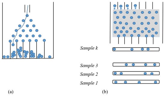
Figure 1. (a) Classical Galton’s board; (b) quantum Galton’s board (Quantum Boson Sampling Machine (QBSM)) [69].

2.2. The Conception of Boson Sampling and Its Mathematical Models

Boson Sampling, which is a nonuniversal version of quantum computation, was introduced by Aaronson and Arkhipov (AABS) [29] and is the first procedure to show quantum supremacy [37] decisively, which means it demonstrates the advantage of quantum computation compared with computation with classical algorithms. It could offer evidence contradicting the Extended Church–Turing theorem, lacking the requirement for a universal quantum computer [64,65].

In Boson Sampling, N indistinguishable single-photon Fock states are sent to the input positions of an M-port linear optical interferometer, with M = O(N²) dimensions, which means that the number of modes can scale quadratically with the number of photons. The input pattern or the photon distributions at the input can be presented as $\stackrel{\_}{s}!=s_1!s_2!\dots s_M!$, in which $s_i$ specifies the number of photons in the i-th mode of the input, which can only be 0 or 1, and the entire number of incoming photons would be identical to N as follows: ${\displaystyle \sum _{i=1}^M{s}_i=N}$ [64,65,69,70].

The linear optical interferometer consists of beamsplitters and phase shifters and is labeled by an M × M unitary matrix U, which carries out a linear transformation on the input creation operators $a_i^{†}$. The number of photons per output mode could be detected utilizing PNR (photon number resolving) detectors, and the pattern of output photons can be written as $\overline{t}!=t_1!t_2!...t_M!$, where $t_i$ can be any integer, representing the photon numbers in the output mode i, and ${\displaystyle \sum _{i=1}^M{t}_i=N}$ [64,65,69,70].

BS is the sampling process from the output probability distribution [64,65,71,72] and, because of bosonic statistics, the probability of calculating a particular output pattern of a photon is correlated to the permanent (Perm) of an N × N submatrix ($U_{(s,t)}$) of the M × M unitary matrix U attributed to the interferometer. Mathematically, the main task of the Boson Sampler is to calculate the probability of a particular output pattern of photons from the input pattern, which can be calculated as follows [64,65,69,70]:

$$\underset{s\to t}{\mathrm{Pr}(t)}={\displaystyle \frac{{\left|Perm(U_{s,t})\right|}^2}{t_1!\dots t_M!s_1!\dots s_M!}}$$

(1)

$U_{s,t}$ is made from the intersection of the columns and rows of the matrix U, which corresponds to the position of input modes (the columns have been selected by the input modes) and output modes (the rows have been selected by the output modes) of the interferometer, respectively (Figure 2) [65].

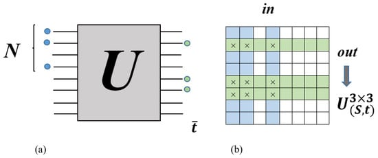
Figure 2. One example of the construction of the sampled submatrix Us based on Aaronson and Arkhipov Boson Sampling (AABS) theory (reproduced with permission from [Kruse, R., Hamilton, C. S., Sansoni, L., Barkhofen, S., Silberhorn, C., & Jex, I.], [Physical Review A]; published by [American Physical Society (APS)], [2019]) [65].

For example, the probability of measuring a certain pattern $(\overline{t})$ in Figure 2, where the number of injected and detected photons in each mode is 0 or 1, is calculated by the square of the permanent $U_{s,t}$ sampled submatrix as follows:

$$\underset{s\to t}{\mathrm{Pr}(t)}={\left|Perm(U_{s,t})\right|}^2$$

(2)

The permanent of an n × n matrix, for example, A, can be generally defined as follows [29]:

$$Per(A)={\displaystyle \sum _{\sigma \in S_n}{\displaystyle \prod _{i=1}^n{a}_{i\sigma (i)}}}$$

(3)

where S_n is the collection of all permutations for the set {1,2,…, n}. The calculation of the permanent of a matrix is in the category of #P-hard counting problems and therefore it is difficult to compute by a classical computer. So the calculation of probabilities of all outputs and sampling from the interferometer output cannot be performed professionally using a classical machine [29,64,65,69,70,71]. The problems are divided into two categories: “decision problems”, where the answers to the problem instances are what is more “yes” or “no”, and “counting problems”, which ask, “How many answers exist?”. The #P class (sharp P) is one complex class of counting problems in which the number of answers to the problem can be calculated by analyzing the candidate’s answers efficiently [29].

The best-recognized classical algorithm to calculate the permanent of an n × n matrix has been introduced by Ryser [73] and requires O(n²2ⁿ) runtime. However, this time could be reduced to O(n·2ⁿ) while increasing the memory cost and data dependency, and destroying parallelism severely. This algorithm, which is appropriate for parallel computing, was not an efficient algorithm until now, because a lot of experimental samples were required to yield an adequate respectable approximation and, due to the incompetence of the algorithm, performing a particular large-scale problem required a long time. So, the classical simulation of BS through the permanent calculation of a matrix requires exponential classical resources [69,70,72].

Boson Sampling experiments have some limitations: (1) They are limited to a small number of indistinguishable single photons in a few modes because of the probabilistic process of single photon generation. (2) The required time to produce single photons in many modes simultaneously increases exponentially as the number of modes increases. (3) It may not be possible to sample the precise distribution of photons because the photon distributions may not be as accurate as designed. (4) The parameters of the optical devices may be somewhat different from the required ones. (5) The detectors cannot indicate the exact number of photons and can only recognize the presence or absence of photons by 1 or 0. So they are not impeccably efficient. Therefore, to overcome the limitations of BS and develop the performance of the BS machines, researchers have introduced more innovative sampling methods based on the nature of photon generation, such as Gaussian Boson Sampling (GBS), to show a computational advantage over classical computers [29,69,70].

2.3. The Conception of Gaussian Boson Sampling and Its Mathematical Models

Since the production of many indistinguishable single photons is limited in the BS method, Hamilton et al. [64] proposed to replace the Fock input states with Gaussian input states, which are more easily produced in large sizes, to solve the Boson Sampling scalability problem. This method is called Gaussian Boson Sampling, in which multimode Gaussian input states, as the nonclassical input states (quantum states), generated deterministically through spontaneous parametric down-conversion, have been injected into the multimode linear interferometer and then measured on Gaussian states using the Fock basis through the photon numbers in the output by using PNR detectors. Sampling from the output probability distribution needs exponential time utilizing classical computers and is in the complexity class #P [6,33,60,64,74].

It should be noted that qumodes are the fundamental physical systems of importance. Unlike qubits, which are shown by a two-dimensional Hilbert space and could be expressed as $\left|\psi \right.⟩=c_0\left|0\right.⟩+c_1\left|1\right.⟩$ such that ${\left|c_0\right|}^2+{\left|c_1\right|}^2=1$, qumodes have been characterized mathematically via a Hilbert space of unlimited dimension and can be defined as $\left|\psi \right.⟩={\displaystyle \sum _{n=0}^{\infty }{c}_n\left|n\right.⟩}$, where ${\displaystyle \sum _{n=0}^{\infty }{\left|c_n\right|}^2=1}$. The Fock states are recognized as the basis states $\left|0\right.⟩,\left|1\right.⟩,\left|2\right.⟩,\dots$, and the physical explanation of a qumode with n photons is identified by the Fock state $\left|n\right.⟩$ [6].

The quantum system state, which has M qumodes, is exclusively known by a quasi-probability distribution called Wigner function W(q, p) [75,76], in which q and p are its position and momentum variables, respectively. If the Wigner function of a quantum state is a Gaussian distribution, it is called a Gaussian state [6,10,66,74]. A Gaussian state with an M mode could be pronounced by a covariance matrix V (2M × 2M dimension) and the position and momentum mean vectors $\stackrel{\_}{q}$ and $\stackrel{\_}{p}$ which are two M-dimensional vectors. However, the covariance matrix is often more appropriately expressed in terms of the complex amplitudes $\alpha ={\displaystyle \frac{1}{\sqrt{2}\hslash }}(q+iP)$ which are complex normal distributed using covariance matrix σ and mean $\overline{\alpha }={\displaystyle \frac{1}{\sqrt{2}\hslash }}(\stackrel{\_}{q}+i\stackrel{\_}{P})$ [6,66,77]. In other words, a Gaussian state could be described through a displacement vector d and a 2M × 2M covariance matrix σ, in which the covariance matrix elements are ${\sigma }_{ij}={\displaystyle \frac{1}{2}}⟨\left\{{\widehat{\xi }}_i,{\widehat{\xi }}_j\right\}⟩-d_i{d}_j$ and $d_j=⟨{\widehat{a}}_j⟩$ [64,65,78,79], where ${\widehat{\xi }}_i$ executes on all creation and annihilation operators ${\widehat{a}}_j$ and ${\widehat{a}}_j^{†}$ of a photon in mode j, which for j = 1, 2, …, M, the following equation holds: ${\widehat{\xi }}_j={\widehat{a}}_j=({\widehat{x}}_j+i{\widehat{p}}_j)/\sqrt{2}$ and ${\widehat{\xi }}_{M+j}={\widehat{a}}_j$ [10,64].

An ideal pure Gaussian state could be produced from the vacuum via an arrangement of single-mode squeezed states, single-mode displacement operations, and M-mode linear optical interferometry [6,33,76,80]. So, contrary to inputs of BS that are single photons, GBS uses squeezed vacuum states as inputs, where $S(r_j)=\exp \left[r_j(a_j^{†2}-a_j^2)/2\right]$ is the squeezing gate, and by applying this gate to the vacuum, a squeezed state can be ready [6,74]. In this equation, r_j is the input squeezing parameter in the jth mode. $D({\alpha }_j)=\exp ({\alpha }_j{a}_j^{†}-{\alpha }_j^{*}{a}_j)$ is a displacement gate, which, for a Gaussian state with zero mean $(\overline{\alpha }=0)$, produced by only single-mode squeezing and then linear interferometry, the displacement is zero (displacement: the operation that produces a coherent state from the vacuum [81]). Also, linear optical interferometry in M mode with unitary matrix U can act on operators as follows: $a_j\to a_j^{\prime }={\displaystyle \sum _j{U}_{ij}{a}_j}$ [6,64,74].

Therefore, for an M-mode Gaussian state without displacement, and 2M × 2M covariance matrix σ, the Gaussian Boson Sampling distribution or the probability of observing Pr(S), a particular output pattern of photons, $S=(s_1,s_2,\dots ,s_M)$, based on photon counting detectors, can be calculated via the following equation, where $s_j$ identifies the number of photons detected in the j–th output mode and the summation of detected photons can be equal to N, ${\displaystyle {\sum }_{j=1}^M{s}_j}=N$ [6,64,80]:

$$\mathrm{Pr}(S)={\displaystyle \frac{1}{\sqrt{\det ({\sigma }_Q)}}}{\displaystyle \frac{Haf(A_S)}{s_1!s_2!\dots s_M!}}$$

(4)

where

$${\sigma }_Q=\sigma +{{\rm I}}_{2M}/2$$

(5)

$$A=X_{2M}[{{\rm I}}_{2M}-{\sigma }_Q^{-1}]$$

(6)

$$X_{2M}=\left[\begin{array}{cc}0& {{\rm I}}_M\\ {{\rm I}}_M& 0\end{array}\right]$$

(7)

According to the above equations, the sampling matrix A, which is a 2M × 2M symmetric matrix (A = A^t), can be written as the following formula:

$$A=\left[\begin{array}{cc}0& {{\rm I}}_M\\ {{\rm I}}_M& 0\end{array}\right]\left[{{\rm I}}_{2M}-{(\sigma +{{\rm I}}_{2M}/2)}^{-1}\right]$$

(8)

I_2M is known as the 2M × 2M identity matrix. These equations show that ${\sigma }_Q$ and A have been obtained using the covariance matrix σ of the Gaussian state [6,64,65,80]. The sampling matrix $A=\left(\begin{array}{cc}B& C\\ C^t& B^{*}\end{array}\right)$, a combination of the thermal (B = 0, C ≠ 0) and squeezed (C = 0, B ≠ 0) contributions, is composed of a two-block symmetric matrix B (M × M) and a two-block Hermitian matrix C (M × M), which belong to the input Gaussian state and depend on the conversion U executed by the interferometer [65,80].

The A_s is a submatrix of A (2N × 2N) obtained through the location of the output modes of detected photons (j), contrary to BS, where the structure of the obtained submatrix corresponds to the mode positions of input and output. The A_s structure is created by selecting rows and columns j, and j + M of A when s_j = 1. The rows and columns j and j + M are removed from A if s_j = 0, and repeated s_j times when s_j > 0 [6,65,80] (Figure 3) [65].

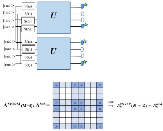
Figure 3. One example of the construction of the submatrix A_S from the state matrix A for two photons detected in two output modes 1 and 4 of an M = 4 mode interferometer in the GBS procedure [65]. (Reproduced with permission from [Kruse, R.; Hamilton, C.S.; Sansoni, L.; Barkhofen, S.; Silberhorn, C.; Jex, I. A detailed study of Gaussian boson sampling. Phys. Rev. A 2019, 100, 032326.]).

For instance, the matrix A with M = 3 modes is a 6 × 6 matrix as follows:

$$A=\left[\begin{array}{cc}{A}_{11}& A_{12}\\ A_{21}& A_{22}\end{array}\right]$$

(9)

where each block $A_{ij}$ is a 3 × 3 submatrix containing the relevant mode interactions.

If the photon pattern is S = (3, 0, 1), the first (1) and fourth (1 + 3) rows and columns of the matrix A are repeated three times, and the second (2) and fifth (2 + 3) columns are removed, and the third (3) and sixth (3 + 3) columns of A repeated once. Therefore, the resulting matrix, A_s, which is an 8 × 8 matrix (2N × 2N with N = 4), can be written as follows [66]:

$$A_s = \left[\begin{array}{cc}\begin{array}{cccc}{a}_{11}& a_{11}& a_{11}& a_{13}\\ a_{11}& a_{11}& a_{11}& a_{13}\\ a_{11}& a_{11}& a_{11}& a_{13}\\ a_{31}& a_{31}& a_{31}& a_{33}\end{array}& \begin{array}{cccc}{a}_{14}& a_{14}& a_{14}& a_{16}\\ a_{14}& a_{14}& a_{14}& a_{16}\\ a_{14}& a_{14}& a_{14}& a_{16}\\ a_{34}& a_{34}& a_{34}& a_{36}\end{array}\\ \begin{array}{cccc}{a}_{41}& a_{41}& a_{41}& a_{43}\\ a_{41}& a_{41}& a_{41}& a_{43}\\ a_{41}& a_{41}& a_{41}& a_{43}\\ a_{61}& a_{61}& a_{61}& a_{66}\end{array}& \begin{array}{cccc}{a}_{44}& a_{44}& a_{44}& a_{46}\\ a_{44}& a_{44}& a_{44}& a_{46}\\ a_{44}& a_{44}& a_{44}& a_{46}\\ a_{64}& a_{64}& a_{64}& a_{66}\end{array}\end{array}\right]$$

(10)

Also, Equation (4) displays that the probability of the output distribution of photons is correlated to the hafnian of A_s (Haf (A_s)), in which the matrix function Haf(.) can be defined as follows:

$$Haf(A)={\displaystyle \sum _{\mu \in PMP(n)}{\displaystyle \prod _{(i,j)\in \mu }{a}_{ij}}}$$

(11)

The elements of A are a_ij, and PMP(n) is defined as the collection of perfect matching permutations of n objects in where n is even (hafnian for odd N is zero). For instance, the collection of perfect matchings for n = 4 is PMP(4) = {(0,1)(2,3), (0,2)(1,3), (0,3)(1,2)} [82,83]. The hafnian is a generalization of the permanent, and the relationship between the permanent and the hafnian for any matrix G is as follows [6,64,65,66]:

$$Haf\left(\begin{array}{cc}0& G\\ G^T& 0\end{array}\right)=Per(G)$$

(12)

To investigate more details of the structure of GBS with squeezed states, the Gaussian Boson Sampling schematic shown in Figure 4 is considered. When K single-mode squeezed states (SMSSs) (K ≤ M) are inserted into an M-mode Haar random unitary linear interferometer U_GBS, all M modes are measured, and the photons in each mode are counted at the output. The matrix A corresponds to the single-mode squeezed states as input, and the linear interferometer has C = 0 and B ≠ 0, where the single-mode squeezed state can be defined by the following matrix [64,65]:

$$S=\left(\begin{array}{cc}{{\displaystyle \oplus }}_{j=1}^M\cosh r_j& {{\displaystyle \oplus }}_{j=1}^M\sinh r_j\\ {{\displaystyle \oplus }}_{j=1}^M\sinh r_j& {{\displaystyle \oplus }}_{j=1}^M\cosh r_j\end{array}\right)$$

(13)

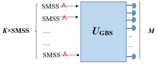
Figure 4. Representation of the GBS procedure. K single-mode squeezed states (SMSSs) have been sent into a Haar random linear interferometer U_GBS of size M and at the output the multimode squeezed state in the Fock state basis has been measured (reproduced with permission from [Kruse, R., Hamilton, C. S., Sansoni, L., Barkhofen, S., Silberhorn, C., & Jex, I.], [Physical Review A]; published by [American Physical Society (APS)], [2019]) [65].

In the above equation, ${{\displaystyle \oplus }}_{j=1}^M{x}_j$ represents a straight summation of numbers that produce a diagonal matrix and can be written as ${{\displaystyle \oplus }}_{j=1}^M{x}_j=diag(x_1,x_2,\dots ,x_M)$. Also, there are at least K nonzero squeezing parameters (r_j), and the zero squeezing parameter (r_j = 0) for the remaining M − K ports (if K ≠ M) relates to vacuum states [64,65].

At the output of the interferometer, the covariance matrix is defined as follows [64,65]:

$${\displaystyle \frac{1}{2}}\left(\begin{array}{cc}{U}_{GBS}& 0\\ 0& U_{GBS}^{*}\end{array}\right)S{S}^{†}\left(\begin{array}{cc}{U}_{GBS}^{†}& 0\\ 0& U_{GBS}^t\end{array}\right)$$

(14)

The matrix A can be defined as $A=B\oplus B^{*}$, where B is an M × M symmetric matrix as follows [64,65,74,80]:

$$B=U_{GBS}\left({{\displaystyle \oplus }}_{j=1}^M\tanh r_j\right)U_{GBS}^t=U_{GBS}diag(\tanh r_1,\dots ,\tanh r_M)U_{GBS}^t$$

(15)

So, according to Equation (4), the probability of the output distribution can be defined as the product of the hafnians of the two submatrices B_s, where B_s is a submatrix of A_s that is obtained only concerning the rows and columns j where a photon was detected, not j and j + M [6,64,65,74]:

$$\mathrm{Pr}(S)={\displaystyle \frac{1}{\sqrt{\det ({\sigma }_Q)}}}{\displaystyle \frac{{\left|Haf(B_s)\right|}^2}{s_1!s_2!\dots s_M!}}={\displaystyle \frac{1}{{\displaystyle \prod _{\mathrm{j}=1}^{\mathrm{M}}{\cos \mathrm{hr}}_{\mathrm{j}}}}}{\displaystyle \frac{{\left|Haf(B_s)\right|}^2}{s_1!s_2!\dots s_M!}}$$

(16)

This probability for 0 or 1 per mode can be simplified as follows [64]:

$$\mathrm{Pr}(S)={\displaystyle \frac{1}{\sqrt{\det ({\sigma }_Q)}}}{\left|Haf(B_s)\right|}^2$$

(17)

B_s is an even-sized matrix and correlated to detect an even number of photons. If the number of detected photons is odd, the distribution probability is zero, and in this case, Equation (4) still holds, but Equation (17) is unacceptable [64,65].

The total mean photon number in the distribution has been calculated by the following equation, which shows that the mean number of photons is correlated to the squeezing parameter [74]:

$$\overline{n}={\sum }_{j=1}^M{\displaystyle \frac{{\sigma }_j^2}{1-{\sigma }_j^2}} ; {\sigma }_j=\tanh \left(r_j\right) ; 0 {\le \sigma }_j<1$$

(18)

In the case of GBS, where that threshold detector has been used instead of the PNR detector, only the location of the detected photon is important, and will “click” when one or more photons are observed in jth mode, which in this case, s_j = 1 and s_j = 0 when no photons are detected in jth mode. The probability of the GBS output distribution is obtained by the following equation, where Tor(.) is the Torontonian function [6,10,84,85] which is detailed in Ref. [84]:

$$\mathrm{Pr}(S)={\displaystyle \frac{Tor(O_s)}{\sqrt{\det ({\sigma }_Q)}}} ; O_s=1-{\sigma }_Q^{-1}$$

(19)

Consequently, the GBS protocol correlates with the hafnian function where the hafnian is permanent and belongs to the #P complexity class, and the time required to run the best algorithms to compute hafnians and Gaussian Boson Sampling scales as N³2^N/2 (N = the size of the matrix) [65,86,87] and increases exponentially with the dimension of the input matrix [66,82]. Therefore, it is not probable to sample the output distribution of a GBS device using classical computers [6,64,65,66].

2.4. The Conception of Bipartite Gaussian Boson Sampling

Bipartite Gaussian Boson Sampling, as described in Figure 5, is a particular protocol of Boson Sampling, and the output distribution depends on not just a symmetric matrix, but also an arbitrary transition matrix. In this strategy, photons have been generated using two-mode squeezing gates to modes j and j + M for j = 1, 2,..., M, which has been defined as $S_2\left(r_j\right)=\mathrm{e}\mathrm{x}\mathrm{p}\left[r_j\left(a_j^{†}{a}_{j+M}^{†}-a_j{a}_{j+M}\right)\right]$ which can be broken into two single-mode squeezing gates with equal parameters (r_j = r_j + M) and a 50:50 beamsplitter. In this protocol, Equation (15) can be changed as follows:

$$B_{BipartiteGBS}=Udiag(\tanh r_j,\dots ,\tanh r_M) V^T$$

(20)

where the complicated notation, $B_{BipartiteGBS}$, has been simplified and represented as B. A unitary interferometer U applies to the first m modes, and another unitary interferometer V applies to the other half of the modes. The distribution of output can be computed in terms of the transition matrix B. If photon numbers in mode j and j + M are shown with s_j and t_j (j = 1,2,…, M), respectively, the notation (S; T) = (s₁,…, s_M; t₁,…, t_M) denotes a sample and the GBS distribution can be defined as follows:

$$\mathrm{Pr}\left(S;T\right)={\displaystyle \frac{1}{\prod _{j=1}^M\mathrm{c}\mathrm{o}\mathrm{s}\mathrm{h}\left(r_j\right)}}{\displaystyle \frac{{\left|Haf\left(\mathit{B}\right(S,T)\right|}^2}{\prod _j{s}_j! \prod _j{t}_j!}}$$

(21)

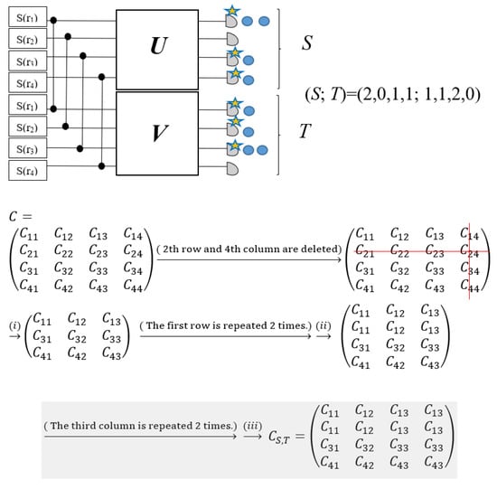
Figure 5. One example of constructing submatrices C_S,T of the Bipartite GBS to encode arbitrary matrices [74]. (Reproduced with permission from [Grier, D.; Brod, D.J.; Arrazola, J.M.; de Andrade Alonso, M.B.; Quesada, N. The complexity of bipartite Gaussian boson sampling. arXiv 2021, arXiv: 2110.06964]).

In the above equation, $\mathit{B}(S,T)$ is a submatrix that corresponds to the notation (S; T), so that when s_j = 0, the jth row of $\mathit{B}$ is deleted and when s_j > 0, it is repeated s_j times. Also, if t_j = 0, the jth column of $\mathit{B}$ is ignored, and if t_j > 0, it is repeated t_j times (Figure 5). The summation of the detected photons in the first half of the modes is identical to the summation of the detected photons in another set of modes, i.e., ${\sum }_{j=1}^M{s}_j={\sum }_{j=1}^M{t}_j=N$, which physically relates to the action of the two-mode squeezing gate, which produces pairs of photons in which every photon in the first m modes has a twin photon in another m modes. Since the permanent is only well defined for square matrices and the above relation is a sign of the square matrices, the output distribution probability of Bipartite GBS is correlated to the permanent function. Based on this opinion, ${\sum }_{j=1}^M{s}_j={\sum }_{j=1}^M{t}_j=N$ and the point that r_j = r_j+M, the number of pairs, considering that the summation only extends to M, can be obtained by

$$⟨n⟩={\sum }_{j=1}^M{\displaystyle \frac{{\sigma }_j^2}{1-{\sigma }_j^2}}$$

(22)

The Bipartite GBS structure is practically like a standard Boson Sampling method [29] because probabilities in both cases are computed based on the permanent of the submatrices created in a similar method. The key difference is that the corresponding matrix describing the interferometer in BS is unitary, while in Bipartite GBS, an arbitrary M × M complex matrix has been employed. Another critical difference is related to the normalization factor Ƶ = $\prod _{j=1}^M\mathrm{c}\mathrm{o}\mathrm{s}\mathrm{h}\left(r_j\right)$. It is crucial to consider the point that the space of outcomes comprises procedures with various total photon numbers, and it will affect the behavior of errors in the ultimate result [74].

3. The Relationship Between Gaussian Boson Sampling and Graph Theory

3.1. Boson Sampling, Gaussian Boson Sampling, and Perfect Matchings in Graph Theory

In recent years, some studies have been performed that show that BS and GBS are related to graph theory [10,88,89,90,91]. This is because the permanent that must be computed in Boson Sampling counts the perfect matching numbers in a bipartite graph, and the hafnian that should be computed to calculate the output probability of GBS counts the perfect matching numbers in a general graph, not necessarily a bipartite graph. So, the hafnian function is greater overall compared with the permanent function, which has been expressed in Equation (12), and G in Equation (12) is attributed to the adjacency matrix of a graph. Therefore, any algorithm that can compute the hafnian exactly could compute the permanent too, both of which are classified as #P-hard problems, even just to calculate the approximate answer [29,64,65,92].

A perfect matching of a graph is a subgroup of the edges where each vertex in the graph is attached to a single unique other vertex by an edge, or no two edges share a vertex. Figure 6 shows two instances of perfect matchings in two graphs in which every vertex is matched up with another vertex [6,82,93,94].

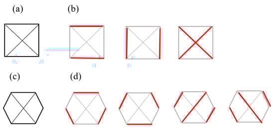
Figure 6. Three perfect matchings (b) of a complete graph with four vertices (a) (Brádler, K., Dallaire-Demers, P. L., Rebentrost, P., Su, D., & Weedbrook, C.], [Physical Review A]; published by [American Physical Society (APS)], [2018]) [93]. Four perfect matchings (d) of a graph with six vertices (c) [94].

According to Figure 7, which explains the connection between Boson Sampling and graphs, to calculate the probability of an output, all probable pathways from input photons to the output that relate to the interferometer must have been considered. In fact, in single-photon Boson Sampling, all paths could be designated through all perfect matchings of a bipartite graph of U_s,t (Equation (1)) where input modes, s, and output modes, t, are vertex sets of a bipartite graph and the edges are the paths between them [95].

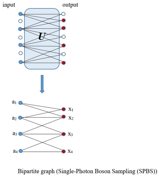
Figure 7. One example of the construction of a bipartite graph from the input (blue dots) and output (red dots) photon configuration of the Boson Sampling procedure (reproduced with permission from [Oh, C., Lim, Y., Fefferman, B., & Jiang, L.], [Physical Review Letters]; published by [American Physical Society (APS)], [2022]) [95].

Two vertices of a symmetric graph of B_s (Equation (17)) form an edge when the two photons originate from an identical source. So, in GBS, to calculate a probability, all feasible perfect matchings of output photons, which relate to finding sources from which each pair of photons arises, have been considered. Therefore, for the limited connectivity of a unitary matrix, the perfect matching number of each output is small, and the corresponding graph structure decreases the complexity [95].

Predicting the number of perfect matchings when the size of the graph increases is hard for a classical computer. In addition, it is acknowledged that the number of perfect matchings of a graph is identical to the hafnian of the adjacency matrix of a graph. So, according to Equations (4) and (17), it will be possible to guess the number of perfect matchings by calculating the photon number distribution probability [92,93]. Also, Equation (17) shows that if the number of perfect matchings in a subgraph increases, its corresponding sample could be outputted through GBS via a greater probability [88].

The adjacency matrix of an undirected and unweighted graph G = (V, E), where V and E signify the collection of vertices and edges, respectively, can be signified by a symmetric matrix A with a ׀V׀ dimension in which diagonal elements of the matrix are zero and other elements are one (A_ij = 1) if there exists an edge between the vertices of i and j and otherwise, it is zero [82,92,93]. So, a great size adjacency matrix generally has a great hafnian. For instance, a complete graph that has 2M vertices has (2M−1)!! perfect matchings. Naturally, if A is simply considered as an adjacency matrix, Equation (4) does not hold for the reason that the probability is smaller than one. To make it reasonable, the adjacency matrix must be rescaled by a small number [93].

3.2. How to Encode Graphs into the GBS Device to Find a Dense Subgraph

A quantum computer is usually encoded by identifying an arrangement of fundamental gates. GBS is constructed from prespecified squeezing, linear interferometry, and displacement gates, and its parameters specify the Gaussian state to be sampled. In pure-state GBS with zero displacements, identifying the parameters of the gate is comparable to identifying the symmetric matrix B (Equation (17)) [6]. With the aim of associating B with the symmetric and positive confident covariance matrix (2M-dimensional) of an M-mode Gaussian state, a “doubled adjacency matrix” should be constructed as the following equation by an appropriate rescaling factor c in which 0 < c < 1/s_max and s_max are the maximum eigenvalue of B:

$$A=c\left(\begin{array}{cc}B& 0\\ 0& B\end{array}\right)=\left(\begin{array}{cc}cB& 0\\ 0& cB\end{array}\right)=c(B\oplus B)$$

(23)

For simplicity, it will be assumed that c = 1 and so A = (B + B) can be encoded into a GBS device, which is called the “doubled encoding strategy” [83,90].

In other words, according to Equation (15), any symmetric adjacency matrix B corresponding to a graph could be encoded into a GBS device via tuning the U and r_i values and through rescaling the matrix through parameter c, which controls the ${\sigma }_j$ values (Equation (18)) and consequently the squeezing parameters r_j and the mean photon number $\overline{n}$ [6,80]. In such a situation, Takagi–Autonne factorization [81,96,97] can decompose the adjacency matrix of a graph as follows:

$$B=Udiag(c{\sigma }_1,\dots ,c{\sigma }_M)U^t ; {\sigma }_j=\tanh \left(r_j\right) ; 0 {\le \sigma }_j<1$$

(24)

and therefore, the associated GBS setup can be created.

Generally, the programming of a GBS device is as follows:

• Determination of the unitary interferometer matrix U and the ${\sigma }_1,\dots ,{\sigma }_M$ values via the computation of the Takagi–Autonne decomposition of B.
• Programming the linear interferometer consistent with the unitary U.
• Solving parameter c so that $\overline{n}={\sum }_{j=1}^M{\displaystyle \frac{{\left(c{\sigma }_j\right)}^2}{1-{\left(c{\sigma }_j\right)}^2}}$
• Programming the squeezing parameter r_j of the squeezing gate S(r_j) acting on the j-th mode so that $r_j={\tanh }^{-1}\left(c{\sigma }_j\right)$

After embedding B via A into the GBS device, GBS can sample from a distribution as follows [6,83]:

$$\mathrm{Pr}\left(S\right)\propto c^N{\displaystyle \frac{{\left|Haf\left(B_s\right)\right|}^2}{s_1!,\dots ,s_M!}} ; N={\sum }_j{s}_j$$

(25)

where B_S is the adjacency matrix correlated to the subgraph of B selected by S, and Haf (B_s) is identical to the number of perfect matchings in this subgraph [10].

Consequently, through embedding the adjacency matrix B into GBS, the obtained sampler can favorably sample results correlating to a subgraph in which the number of perfect matchings is great. This means that the GBS device can sample large hafnian subgraphs with a high probability. The number of edges in a graph divided by the number of edges in the complete graph is defined as the density of a graph. A large number of perfect matchings in a subgraph makes the subgraph have a large density. So, the programmed GBS devices can sample dense subgraphs with a great probability [10,92]. Hence, GBS with SMSV states, in addition to proving a quantum advantage in sampling tasks, is of interest for applications in graph problems, such as finding dense subgraphs, the max clique [88], and graph similarity [80,83].

Therefore, by combining Gaussian Boson Sampling, random sampling, and classical random optimization algorithms, quantum–classical hybrid optimization algorithms have been constructed, which are used to identify dense subgraphs or maximum cliques in a graph [10,92].

Graphs were applied to consider an extensive range of models, for instance, websites [98], financial markets [99], social networks [100], and biological networks [101]. For graph G with n vertices, the dense subgraph problem is defined as finding its subgraph with k vertices (k < n), G_s, with the highest density, $W\left(G_s\right)$, that contains a great number of edges between its vertices, which are extremely attached [90].

$$W\left(G_s\right)=\left|{\sum }_{i,j=1}^k{\left(A_s\right)}_{i,j}\right|$$

(26)

The adjacency matrix of G_s is shown with A_s.

Finding the dense subgraph is important whenever recognizing such important correlations in proteins in a biological system or social network is important [6,90].

A clique in a graph is a complete graph that has a unit density and is defined as a subgraph that comprises all possible edges between its vertices. Finding the greatest clique in a graph is well known as the maximum clique problem, which can be identified via finding a submatrix B_s from the matrix B with the largest hafnian in the square of absolute value. The max clique problem is in the category of NP-hard complexity class problems [67]. The new applications of the max clique problem are in the fields of social network analysis [102], bioinformatics [103], flight scheduling [104], telecommunications [105], and finance [6,90,106]. Figure 8 shows a general schematic of the connection between GBS and a graph, and encoding a graph into a GBS device to find the cliques [90,107].

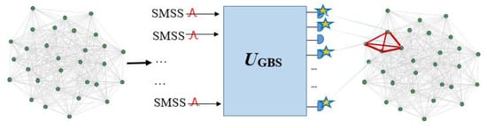
Figure 8. A general schematic of the connection between GBS and a graph and encoding a graph into a GBS device to find the cliques. Each vertex of the graph corresponds to an output mode of the GBS, and the detected output modes indicate a four-vertice subgraph which is marked in red [92,107]. (Reproduced with permission from Yu, S.; Zhong, Z.-P.; Fang, Y.; Patel, R.B.; Li, Q.-P.; Liu, W.; Li, Z.; Xu, L.; Sagona-Stophel, S.; Mer, E.; et al. A universal pro-grammable gaussian boson sampler for drug discovery. arXiv 2022, arXiv: 2210.14877).

According to the definitions of a dense subgraph and max clique, it is concluded that a dense subgraph is not necessarily a maximum clique, but a maximum clique is a dense subgraph. Also, since the GBS samples have a greater hafnian, subgraphs correlated to the GBS samples have a greater hafnian. So, the GBS samples, by increasing their success probability, have been used to increase the efficiency of stochastic algorithms in explaining the max haf problem. In addition, because graph density is correlated to the hafnian, dense subgraph problems can be effectively solved via GBS too [88,90]. The difference between the dense subgraph and max clique problems is due to their objective functions’ computational difficulty. The computation of the hafnian is hard, whereas the evaluation of density is efficient. The study of the two graph problems offers us insights that show that GBS is effective in solving the computational complications of the graph feature [90].

4. Graphs That Can Be Embedded in the X8 Photonic Chip

As mentioned, GBS is presently one of the NISQ methods that is usable to solve some problems, including graph problems. Gaussian Boson Sampling can be performed on the X8 photonic chip provided by Xanadu, which is available on the Xanadu cloud. Studying the embedding of graphs into the X8 chip to perform different operations, for instance, graph similarity [83] and graph isomorphism [89], which has a significant role in graph classification, is one of the works that is performed on the photonic chip. Encoding graphs into the X8 hardware is beneficial for obtaining informative features and solving machine learning problems.

In a previous study [108], the graphs that can be embedded on the X8 photonic device and how isomorphism properties can be extracted from them, considering the X8 hardware constraints, have been investigated. For this purpose, the implemented circuit on X8 hardware is shown in Figure 9 [60]. This circuit consists of eight input modes in the vacuum state, and S2 gates are applied between the first four modes (signal) and the second four modes (idler), for which, after applying a unitary transformation on each of the two groups, the photons are ultimately detected at the output and the measurement is completed by counting the number of photons in each mode.

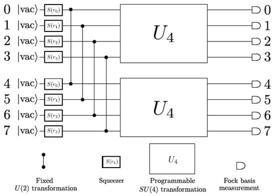
Figure 9. X8 chip quantum circuit diagram [60]. (Reproduced with permission from [Arrazola, J.M.; Bergholm, V.; Brádler, K.; Bromley, T.R.; Collins, M.J.; Dhand, I.; Fumagalli, A.; Gerrits, T.; Goussev, A.; Helt, L.G.; et al. Quantum circuits with many photons on a programmable nanophotonic chip. arXiv 2021, arXiv: 2103.02109]).

The graphs in which the number of vertices of graphs is identical to the number of modes of the hardware can be encoded in X8 hardware via an adjacency matrix A that has been associated with the graph. So, graphs with eight vertices and with the following conditions, (1) unweighted (the matrix elements are 0 or 1), (2) undirected (the symmetric matrix), (3) the diagonal of the matrix is 0, can be encoded in X8 hardware. Hence, the 8 × 8 adjacency matrix A that satisfies the above conditions has 28 independent parameters, in which $a_i=0 or 1$, and the number of graphs in this condition is 2ⁿ, i.e., 2²⁸ = 2.68 × 10⁸.

$$A=\left[\begin{array}{cc}\begin{array}{cc}\begin{array}{cc}0& a_0\\ a_0& 0\end{array}& \begin{array}{cc}{a}_1& a_2\\ a_7& a_8\end{array}\\ \begin{array}{cc}{a}_1& a_7\\ a_2& a_8\end{array}& \begin{array}{cc}0& a_{13}\\ a_{13}& 0\end{array}\end{array}& \begin{array}{cc}\begin{array}{cc}{a}_3& a_4\\ a_9& a_{10}\end{array}& \begin{array}{cc}{a}_5& a_6\\ a_{11}& a_{12}\end{array}\\ \begin{array}{cc}{a}_{14}& a_{15}\\ a_{18}& a_{19}\end{array}& \begin{array}{cc}{a}_{16}& a_{17}\\ a_{20}& a_{21}\end{array}\end{array}\\ \begin{array}{cc}\begin{array}{cc}{a}_3& a_9\\ a_4& a_{10}\end{array}& \begin{array}{cc}{a}_{14}& a_{18}\\ a_{15}& a_{19}\end{array}\\ \begin{array}{cc}{a}_5& a_{11}\\ a_6& a_{12}\end{array}& \begin{array}{cc}{a}_{16}& a_{20}\\ a_{17}& a_{21}\end{array}\end{array}& \begin{array}{cc}\begin{array}{cc}0& a_{22}\\ a_{22}& 0\end{array}& \begin{array}{cc}{a}_{23}& a_{24}\\ a_{25}& a_{26}\end{array}\\ \begin{array}{cc}{a}_{23}& a_{25}\\ a_{24}& a_{26}\end{array}& \begin{array}{cc}0& a_{27}\\ a_{27}& 0\end{array}\end{array}\end{array}\right]$$

Due to the X8 hardware limitations, the graphs that can be encoded in X8 are restricted based on the bipartite graphs, signal and idler mode constraint, and normalization constraint, which are described below.

Because of the X8 structure, only the bipartite graphs that cause identical squeezing on all modes can be implemented on X8 chips. This limitation will be addressed one day with the development of the chip and new generations of chips [108,109]. The adjacency matrices of the graphs with this restriction can be shown as follows, in which M is a 4 × 4 submatrix. In this situation, the number of parameters would be decreased to 16, and consequently, the number of graphs to 65,536.

$$A=\left[\begin{array}{cc}0& M\\ M^T& 0\end{array}\right]=\left[\begin{array}{cc}\begin{array}{cc}\begin{array}{cc}0& 0\\ 0& 0\end{array}& \begin{array}{cc}0& 0\\ 0& 0\end{array}\\ \begin{array}{cc}0& 0\\ 0& 0\end{array}& \begin{array}{cc}0& 0\\ 0& 0\end{array}\end{array}& \begin{array}{cc}\begin{array}{cc}{a}_0& a_1\\ a_4& a_5\end{array}& \begin{array}{cc}{a}_2& a_3\\ a_6& a_7\end{array}\\ \begin{array}{cc} a_8& a_9\\ { a}_{12}& a_{13}\end{array}& \begin{array}{cc}{a}_{10}& a_{11}\\ a_{14}& a_{15}\end{array}\end{array}\\ \begin{array}{cc}\begin{array}{cc}{a}_0& a_4\\ a_1& a_5\end{array}& \begin{array}{cc}{a}_8& a_{12}\\ a_9& a_{13}\end{array}\\ \begin{array}{cc}{a}_2& a_6\\ a_3& a_7\end{array}& \begin{array}{cc}{a}_{10}& a_{14}\\ a_{11}& a_{15}\end{array}\end{array}& \begin{array}{cc}\begin{array}{cc}0& 0\\ 0& 0\end{array}& \begin{array}{cc}0& 0\\ 0& 0\end{array}\\ \begin{array}{cc}0& 0\\ 0& 0\end{array}& \begin{array}{cc}0& 0\\ 0& 0\end{array}\end{array}\end{array}\right]$$

The hardware constraints regarding the connections between the first four modes (the signal modes) of the X8 chip and the four last (the idler modes) also apply a new condition on the submatrix M: it must be symmetric. One can then reduce the number of independent parameters to 10 (1024 possible graphs).

Due to the relations between the signal and idler modes of the X8 chip, hardware limitations will impose new conditions on the M matrix: the M matrix must be symmetric and represented as follows. Consequently, the number of independent parameters is decreased to 10 and therefore the number of possible graphs to 1024.

$$M=\left[\begin{array}{cc}\begin{array}{cc}{a}_0& a_1\\ a_1& a_4\end{array}& \begin{array}{cc}{a}_2& a_3\\ a_5& a_6\end{array}\\ \begin{array}{cc}{a}_2& a_5\\ a_3& a_6\end{array}& \begin{array}{cc}{a}_7& a_8\\ a_8& a_9\end{array}\end{array}\right]$$

The graphs can be named as: “a₀ a₁ a₂ a₃ a₄ a₅ a₆ a₇ a₈ a₉”.

The embedding method is the last restriction executed on the adjacency matrix. The Strawberry Fields (sf) library is used to interconnect with the X8 chip and embed the graphs.

To use the bipartite graph class in Strawberry Fields, an m mean photon per mode normalization parameter is required so that all stages have a squeezing parameter of 1 (r = 1). The only configurations that can be embedded are those in which the squeezing parameter r is the same or equal to zero for all four signal modes, which imposes the following restriction on M:

$$M=U_{diag}\left(tanh{r}_i\right)U^T$$

(27)

This restriction causes the number of embedded graphs to be reduced to 75 graphs.

It is noticed that the value of m is computed by the number of subgraphs of the graph. For n subgraphs (up to n = 4), m = n × m₀. The m₀ is adopted directly from the numerical value reported in the original article [108].

Based on these constraints, the 75 graphs embeddable in X8, most of which are isomorphic, are divided into 10 categories, which have been gathered in Table 1 [108].

Table 1. The 75 graphs which can be embedded in the X8 chip [108]. (Reproduced with permission from [Pierre, E.; Nowak, M. Towards graph classification with Gaussian Boson Sampling by embedding graphs on the X8 photonic chip. arXiv 2021, arXiv:2109.12863]).

Graph	Contains	Number of Graphs	The Matrix Associated with the Graph
1K2, m = m0	a K2 subgraph and 6 free vertices	4
2K2, m = 2m0	2 K2 subgraphs and 4 free vertices	12
1C4, m = m0	a C4 subgraph and 4 free vertices	6
2P3, m = 2m0	2 P3 subgraphs and 2 free vertices	12
3K2, m = 3m0	3 K2 subgraphs and 2 free vertices	16
1K33, m = m0	a K3,3 subgraph and 2 free vertices	4
2S3, m = 2m0	2 S3 subgraphs and no free vertex	4
4K2, m = 4m0	4 K2 subgraphs and no free vertex	10
2C4, m = 2m0	2 C4 subgraphs and no free vertex	6
1K44, m = m0	a K4,4 graph	1

5. The Strawberry Fields Platform Applications

Strawberry Fields, which was introduced by Xanadu, is an important open-source library that has been implemented in Python 3.2 for photonic quantum computing. It is based on the CV (continuous variable) model, is easy to use, and many users can use it. Because near-term quantum computer applications are still under investigation, Strawberry Fields is an important piece of software for solving different problems and is the basis for future photonic quantum computer applications [6,36].

One of the main incentives to manufacture a quantum computer is to use it for real-world applications. Strawberry Fields can be used to program the chips and analyze the output samples for each job and its applications can be classified into four general categories: (1) Graphs and networking, which contains “dense subgraphs” and “maximum clique” problems that have been reviewed in the previous section. (2) Machine learning that includes “graph similarity”, “point processes”, and “training variational GBS distributions” problems. (3) Chemistry which comprises “vibronic spectra”, “vibrational dynamics”, and “vibrational excitations problems”. (4) Sampling where “sampling from GBS” and “pre-generated datasets” are its problems [110].

Machine learning: Strawberry Fields can be used in quantum photonic devices for machine learning. Quantum machine learning is a quickly developing field with numerous methodologies for quantum systems. Quantum circuits have been considered as a neural network analog, which offers a machine learning model via governing gate quantities [110,111].

Chemistry: The simulation of chemical systems, especially when the atomic-level interactions based on quantum mechanics are important, can be performed using quantum computers. Studying light absorption by materials at several frequencies, which can be used in pharmaceuticals or solar cell optimization, and also the optimization of the vibrational excitation of molecules, which can help in designing chemical reactions, are some photonic quantum device applications in the field of chemistry. Strawberry Fields can complete these jobs via the reconstruction of vibronic absorption spectra and the simulation of molecular vibrational excitations and dynamics by entering the chemical quantities of the considered molecule [110,112].

Sampling: Sampling is a common job in quantum computers, which are probabilistic. For example, GBS is known as a photonic algorithm that can be implemented by near-term quantum computers. Graph optimization, chemistry computations, and machine learning are some applications of samples from GBS, in which Strawberry Fields can insert problems into GBS without designing a quantum circuit [110]. A graphic diagram of Strawberry Fields containing the applications layer for photonic quantum computing is displayed in Figure 10.

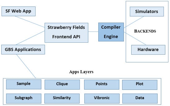
Figure 10. A schematic representation of the Strawberry Fields library [6]. (Reproduced with permission from [Bromley, T.R.; Arrazola, J.M.; Jahangiri, S.; Izaac, J.; Quesada, N.; Gran, A.D.; Schuld, M.; Swinarton, J.; Zabaneh, Z.; Kil-loran, N. Applications of near-term photonic quantum computers: Software and algorithms. arXiv 2019, arXiv: 1912.07634]).

Strawberry Fields comprises two key components: the front-end section to create and compile the quantum programs, and the back-end section to run programs on hardware and simulators. The quantum compiler engine connects the front-end to the back-end and can presently be linked to one of three quantum computer simulators. A new front-end module to implement GBS algorithms is called the GBS applications layer, which focuses on particular GBS applications such as maximum clique, dense subgraph specification, point processes, graph similarity, and vibronic spectra. So, customers interested in a particular topic can focus nearly solely on the correlated module [6,36].

6. Practical Applications of Photonic Quantum Computers Based on GBS

The current applicable quantum computers are NISQ systems, which are weaker than a universal quantum computer, have a restricted number of qubits and imperfect operations, and can only be applied to solve particular problems. Therefore, the specification of problems that can be solved by these devices is very important. GBS, which applies squeezed light to encode and transport the input states and makes scaling easier, displays a pronounced capability to exhibit a quantum advantage in optical systems [37,60] and can be implemented and solved professionally on photonic processors, especially when solving them with classic computers in a reasonable time is challenging [10,107,113]. Recently, several real-world practical applications of GBS, which is a platform for photonic quantum computation, have been reported, for example, the vibrational spectra estimation of molecules [60,112,114,115] and molecular docking [10,107,116]. In the following paragraphs, solving the molecular docking problem and the molecular vibrational problem using Gaussian Boson Sampling has been reviewed.

6.1. Molecular Docking Problems Solved with GBS

One of the most significant applications of GBS is its use in drug design, for instance, protein folding and molecular docking [10,107]. Protein folding, which is simulated generally through appropriate 2D or 3D lattice models such that the interaction energy of amino acids of the protein is minimized, can be displayed as a Hamiltonian problem by accurate encoding procedures so that the ground state displays the structure of the related protein in the particular lattice [25,117]. Recently, studies have been performed on protein folding using quantum annealing [18,118,119,120] or gate-based quantum computation [17,117,121,122], as well as using Gaussian Boson Sampling [107].

Molecular docking, which is an important problem in drug discovery and drug design, is a computational process to guess the best interaction between a drug (small molecule as a ligand) and a receptor (goal macromolecule) which starts from the three-dimensional molecular structures of both components to identify stable ligand–receptor complexes through a potential energy function, which searches the structural space of two molecules and assigns a score to each pose [10,25,123].

The molecular docking output predicts the best three-dimensional orientation of the ligand concerning the receptor binding site and the associated score for each orientation, which requires exact scoring functions (a group of physical quantities that are adequate to score binding orientation and interactions consistent with experimental data) and well-organized search algorithms (an optimization method to achieve the minimum of a scoring function) [10,25].

Numerous methods have been developed with different computational requirements to find stable ligand–receptor structures [10,124,125,126,127].

Molecular docking with classical algorithms often shows restrictions in computational scalability and precision for complex biomolecular structures. Hence, some present studies have concentrated on the practical applications of NISQ systems and Gaussian Boson Sampling in drug design problems, particularly molecular docking [10,107].

GBS can be used to solve the molecular docking problem based on the geometric connection between proteins and ligands. The best docking configuration of the drug–protein structure can be obtained by finding the maximum weighted clique in the correlated binding interaction graph (BIG). A binding interaction graph is a weighted graph created through docking modes between a drug and a protein such that the weighted vertices characterize the possible interaction between the pharmacophores of the drug and the protein, weighted by the contact potential, and the edges characterize the compatible contacts between pairs of vertices. Then, by encoding the adjacency matrix of the BIG into a GBS device, the molecular docking problem can be solved through the finding of the maximum weighted clique in the binding interaction graph [10,107].

By programming the GBS device, GBS can sample from a distribution of the subgraphs with a high weight (close to a clique) with a high probability. The obtained maximum weighted clique with the highest probability is equal to the best docking configuration between the drug and protein. Direct sampling or hybrid algorithms, in which the GBS outputs are post-processed utilizing classical methods, can lead to docking configurations. Indeed, GBS can be used to develop the efficiency of classical algorithms.

In a recent study [10] published by Xanadu on the use of Gaussian Boson Sampling in molecular docking problems, Xanadu’s quantum photonics platform was integrated with classical molecular docking algorithms to increase sampling efficiency by GBS to find the best docking configurations between the TACE (tumor necrosis factor-α converting enzyme) and AS (a thiol-containing aryl sulfonamide ligand) (TACE-AS).

Both the ligand and the binding position of the protein (receptor) are displayed as labeled distance complete graphs, where the vertices of these graphs are pharmacophore points (as a group of points that have an important effect on the molecule’s pharmacological connections [128]), and the distance between these points is shown with edge weights. By combining these two graphs, the corresponding binding interaction graph has been constructed, such that each vertex shows the possible link between the ligand and the protein, weighted by the interaction potential, and each edge displays a pair of vertices that have compatible interactions (Figure 11) [10]. The obtained binding interaction graph is then used to encode in GBS and to solve the molecular docking problem to find the maximum weighted clique, which is in the category of NP-hard problems. The molecular docking configurations are represented as a complete subgraph (clique) of the graph, in which the number of possible subgraphs in an n-vertices graph is O(2ⁿ). The heavyweight cliques show the most likely molecular docking configurations, and the maximum weighted clique in the TACE-AS graph is equivalent to the best ligand–receptor interaction (Figure 12) [10].

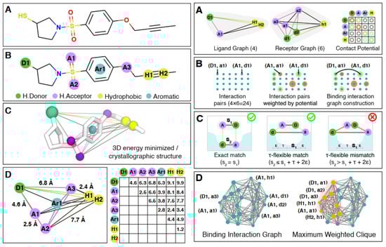
Figure 11. Constructions of the (left) labeled distance graph for the ligand molecule and (right) the binding interaction graph [10]. (Reproduced with permission from [Banchi, L.; Fingerhuth, M.; Babej, T.; Ing, C.; Arrazola, J.M. Molecular docking with Gaussian boson sampling. arXiv 2019, arXiv: 1902.00462v1]).

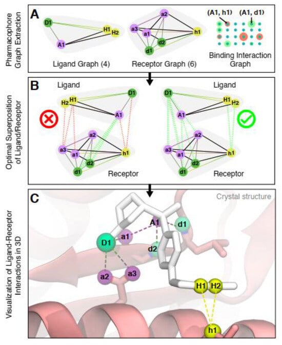
Figure 12. Graph-based molecular docking of an aryl sulfonamide compound to [10]. (Reproduced with permission from [Banchi, L.; Fingerhuth, M.; Babej, T.; Ing, C.; Arrazola, J.M. Molecular docking with Gaussian boson sampling. arXiv 2019, arXiv: 1902.00462v1]).

GBS devices with a very high sampling rate, and by noticing the photon distribution, can extract the maximum weighted clique for small graphs, which is called GBS random search. When squeezed light is inserted into a programmed GBS device, the existence or absence of photons is detected by detectors. Each output port of the GBS where photons were detected corresponds to a vertex of the graph, and therefore, based on the detected output ports, a subgraph is constructed and checked if it is a clique or not. If this subgraph is not a clique, two hierarchy post-processing algorithms (greedy shrinking and local search), which have a long run time but are suitable for finding cliques in larger graphs, have been proposed. Greedy shrinking iteratively deletes a vertex of the GBS random subgraph based on both its degree and its weight until a clique is achieved. In the local search algorithm, the obtained clique from the output of the greedy shrinking algorithm as the input to a local search algorithm has been extended by adding a neighboring vertex to reach a greater clique (Figure 13) [10].

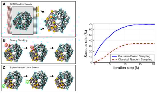
Figure 13. (Left) Schematics of the protocol of GBS algorithms (right) GBS vs. classical success rate [10]. (Reproduced with permission from [Banchi, L.; Fingerhuth, M.; Babej, T.; Ing, C.; Arrazola, J.M. Molecular docking with Gaussian boson sampling. arXiv 2019, arXiv: 1902.00462v1]).

The results of GBS show that the success rate of the algorithm in discovering the maximum weighted clique, which has eight vertices, approximately increases from 30% (classical approach) to 70% (Figure 13) [10]. This hybrid quantum–classical approach also considerably decreases computational costs, enables the quick identification of the best drug–receptor interactions in large chemical libraries, and accelerates drug discovery procedures [10].

In another study [107], published in 2023, a multipurpose quantum drug discovery platform, based on a GBS processor, was implemented for RNA folding prediction and molecular docking problems. In this work, programmable photonic circuits integrate with advanced algorithms to develop a programmable, universal, and software-scalable time-bin-encoded GBS photonic quantum processor to accomplish high-dimensional sampling jobs. This processor has easily modifiable squeezing parameters and can perform arbitrary unitary operations using a programmable interferometer. By applying this device, almost twice the success probability of GBS in comparison to classical sampling to find cliques in a 32-node weighted graph has been demonstrated.

Furthermore, a quantum inverse virtual screening (QIVS) platform has been developed based on GBS to perform molecular docking between PARP (Poly (ADP-Ribose) polymerase-1) and an 8-chloroquinazolinone-based (CQ) inhibitor (PARP-CQ), which forms a 28-vertices BIG, and is a favorable anti-cancer drug [129,130] or a promising drug for some central nervous system (CNS) illnesses, for example, Alzheimer’s and Parkinson’s illnesses [131,132], and also between TACE (tumor necrosis factor (TNF)-α converting enzyme) and TS (thiomorpholine sulfonamide hydroxamate inhibitor) (TACE-TS) [133], which forms a 24-vertices BIG, and are effective in inflammatory illness treatments [134]. By encoding the 28-vertex BIG of PARP-CQ into this device and after post-processing, the sampling results and their associated cliques, along with the weight of each clique and its probability (Figure 14), show that the clique with ten vertices and weight = 6.8144 is the maximum weighted clique, indicating the best connection mode of this complex with a great success rate. Also, performing these steps on the 24-vertex BIG of TACE-TS shows that the maximum weighted clique is a clique with nine vertices and weight = 4.5657 (Figure 14), which is equivalent to the best docking configuration of this complex. Compared with the technique used in Ref [10] (Molecular docking results of TACE-AS complex), the developed procedure in this work produces a more exact molecular docking result.

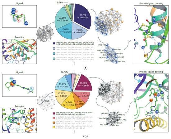
Figure 14. Molecular docking of (a) PARP-CQ complex and (b) TACE-TS complex with GBS [107]. (Reproduced with permission from [Yu, S.; Zhong, Z.-P.; Fang, Y.; Patel, R.B.; Li, Q.-P.; Liu, W.; Li, Z.; Xu, L.; Sagona-Stophel, S.; Mer, E.; et al. A universal pro-grammable gaussian boson sampler for drug discovery. arXiv 2022, arXiv: 2210.14877.]).

The molecular docking results with GBS in a previous study [107] demonstrate that GBS considerably improves the prediction of optimal docking configuration and achieves up to an almost 25% improvement in accuracy compared with classical computational methods and can move toward use in real-world applications.

Also, RNA sequence folding prediction has been successfully performed with the aim of the expansion of nucleic acid drugs through GBS. The RNA sequence has been considered as a Weighted Full Stem Graph (WFSG) where each vertex denotes a probable stem in the sequence in which the weight of each vertex is identical to the distance of the stem, and the co-existence between them is shown as the edges, and then encoded into the programmable GBS device to find the maximum weighted cliques to predict RNA folding prediction [107,135]. In the first case, the folding of an RNA sequence (Accession Number: AH003339) has been predicted by encoding the correlated 32-vertices WFSG in the device, where two maximum weighted cliques have been found, in which the Matthews correlation coefficient (MCC) of the best of them is equal to 0.953, which is better than the MCC values obtained with FOLD (0.864) [136] and RNAProbing (0.934) [137] (Figure 2c in Ref. [107]). In the second case, the corresponding 31-vertex WFSG of an RNA sequence (Accession Number: AB041850) is encoded into the device, and the best configuration corresponding to the maximum weighted clique has an MCC = 1.00, which is more exact than the MCC values obtained with FOLD (0.870) and MCCRNAProbing (0.914) (Figure 2d in Ref. [107]). So, a favorable solution for the real-world applications of NISQ, particularly GBS in the biopharmaceutical industry, has been suggested [107].

6.2. Molecular Docking Problems Solved with QAOA

In another study [25], some molecular docking problems, which could be represented as graphs, have been solved with the quantum approximate optimization algorithm (QAOA) [138], which is a kind of Variational Quantum Algorithm (VQA) [139], to obtain the maximum weighted clique of the given graphs that is equivalent to the best molecular docking interaction.

Variational Quantum Algorithms (VQAs) are hybrid quantum–classical approaches designed to solve optimization problems and simulate quantum systems, which, because of their hybrid quantum–classical nature and their resistance to noise, have been introduced as an important approach to obtain a quantum advantage on NISQ devices [139,140].

VQAs are a quantum version of extremely popular machine learning procedures, for example, neural networks. In VQAs, parametrized quantum circuits (PQCs) run on the quantum computer to estimate the cost function, and then the parameter optimization is implemented on a classical optimizer to minimize the cost function. This approach leads to shallow quantum circuit depth and reduces noise. Therefore, the important parts of VQAs contain a cost function (for encoding problems), PQC (the key portion that distinguishes VQAs from classical neural networks and contains some fixed quantum gates and trainable quantum gates, and could even contain some measurement and feedback processes), and optimization algorithms. VQAs have numerous applications, including finding the ground state in quantum chemistry, quantum approximate optimization algorithms (QAOA) for combinatorial problems, machine learning, and other fields [139,140].

In the aforementioned study [25], three real-world docking problems, such as the SARS-CoV-2 Mpro complex with pyrazoline-based inhibitor PM-2-020B, the DPP-4 complex with piperidine fused imidazopyridine 34, and the HIV-1 gp120 complex with JPIII-048, have been solved with QAOA and digitized counter diabatic (DC)-QAOA (an improved version of QAOA) to obtain the maximum vertex weight clique in the corresponding binding interaction graphs, which indicates the most probable docking position in each complex. In this procedure, a multipart biological problem converts into an optimization problem that can be solved using near-term digital quantum computers, such that the cost Hamiltonian from the mathematical optimization formulations of the maximum vertex weight clique can be derived and solved with QAOA and DC-QAOA, and the optimal docking configuration can be extracted from the ground state. The binding interaction graph for each complex signifies the possible interactions between interacting pharmacophore points, obtained by the integration of the labeled distance graphs of the ligand and protein, and has nm vertices in which n and m are the vertex numbers in the ligand and protein binding site graphs, respectively. So, the molecular docking algorithm based on QAOA requires mn qubits to discover the maximum weighted clique.

For example, the binding interaction graph resulting from the connection of pharmacophore points of PM-2-020B (two) and pharmacophore points of SARS-CoV-2 Mpro (three) has six (2 × 3 = 6) vertices and weights of the vertices in the BIG assigned based on the pharmacophore potential. Therefore, this problem has been solved with six-qubit digital quantum computers, such that the corresponding Hamiltonian of the adjacency matrix (6 × 6) related to the BIG has been solved with QAOA and the DC-QAOA.

Additionally, the molecular docking problem of the DPP-4 complex (effective in the treatment of type 2 diabetes and glucose regulation) with piperidine-fused imidazopyridine 34 (a powerful DPP-4 inhibitor that shows promise in improving glycemic control) has been investigated. Because of two pharmacophore points in the piperidine-fused imidazopyridine 34 ligand and four pharmacophore points in DPP-4, an eight-vertex BIG and consequently an 8 × 8 adjacency matrix has been constructed, and the maximum weighted clique of the graph corresponding to the adjacency matrix has been found using the QAOA and the DC-QAOA methods.

Also, the BIG of the HIV-1 gp120 complex with JPIII-048 (a critical molecular interaction in HIV research) has 12 vertices, because of three pharmacophore points on JP-III-048 and four pharmacophore points on HIV-1 gp120, which causes a 12 × 12 adjacency matrix. Both the common QAOA and the DC-QAOA have been used to find the maximum weighted clique of the graph.

The results obtained from QAOA and DC-QAOA show that DC-QAOA exhibits more efficiency in exactly determining the ground state energy compared with the common QAOA, which leads to greater fidelity in greater molecular docking problems and is more consistent with biological principles, and also shows that quantum computing can offer important insights into the design and optimization of beneficial drugs [25].

These three docking problems have been solved using QAOA and DC-QAOA, not by GBS. So they can be proposed as molecular docking problems that can be solved by Gaussian Bosonic Sampling with 6, 8, and 12 qubits.

6.3. Molecular Vibronic Spectra and GBS

The investigation of molecular vibrational spectra is another application of GBS, which was proposed to solve problems in the field of chemistry, besides molecular docking problems.

Light absorption by molecules occurs at frequencies that relate to the allowable energy transitions between various vibrational and electronic states. In this case, the frequencies and intensities of the absorbed light specify the vibrational spectrum of a molecule. Molecular vibrations are correlated with the stability and reactivity of molecules, the stability of atmospheric materials subjected to vibrational excitation by sunlight [141], and the applications of molecules in photovoltaics or as dyes in industrial developments [6,60,112]. Molecular vibrations are significant in chemical reactions caused by rapid transformations in the electronic state of a molecule. Vibronic transitions occur via light absorption, molecules excite to greater energy electronic states, and the change in electronic state is often along by the vibrational excitations [112,142]. Predicting the vibronic spectra of a molecule or the probabilities of excitation to all vibrational states during transitions, where instantaneous changes in the vibrational and electronic states of molecules occur [143], is challenging via classical approaches. This difficulty arises because the Franck–Condon factors [144], which describe transition amplitudes, typically need exponential time to compute [60].

Photonic algorithms, in which optical modes signify the vibrational normal states of a molecule, use device programming with displacement, squeezing, and linear interferometers to compute the Franck–Condon profiles (mathematical functions that specify the possibility of observing a transition at a given frequency). These algorithms outperform classical methods in predicting vibrational spectra [60,112,115,145]. One application of GBS, which is a photonic algorithm, is the simulation of the vibronic spectra of molecules or the estimation of probabilities of the vibrational transition between ground and excited states of a certain molecule. [114,115,146,147]. When a GBS machine is encoded with suitable molecular quantities, the distribution of vibrational quanta in the molecule throughout a vibronic transition could be obtained by the distribution of photons in the optical modes of the device. The computational complexity of obtaining this information from classical algorithms increases rapidly with increasing molecular size. Consequently, the use of classical algorithms is not appropriate for large molecules. So, the effective simulation of the vibrational excitation of molecules experiencing vibrational transitions can be performed using Gaussian Boson Sampling.

Theoretical Concepts of the Relationship Between Vibrational Spectra and GBS

Based on the Franck–Condon (FC) approximation [144,148], the prediction of the vibrational excitation probabilities as a result of a vibronic transition can be specified by approximating the FC factors for all of the probable transitions that might happen between the vibrational states of the two electronic states. The maximum number of vibrational quanta (K) in all modes, and the number of vibrational modes (M), determine the total number of estimable FC factors, which can be computed by the following equation [112]:

$$n_{FC}={\left(1+{\sum }_{k=1}^K{\displaystyle \frac{\left(M+k-1\right)!}{\left(M-1\right)!k!}}\right)}^2$$

(28)

Also, the FC factor, which identifies the observing probability of an excitation from the state $\left|n\right.⟩$ to the state $\left|m\right.⟩$, can be displayed based on the initial and final vibrational Fock states as follows [112]:

$$F\left(m,n\right)={\left|⟨m\left|{\widehat{U}}_{Dok}\right|n⟩\right|}^2$$

(29)

where $\left|n\right.⟩$ and $\left|m\right.⟩$ denote the number of vibrational quanta in the ground and excited electronic states, respectively.

The Franck–Condon profile (FCP), which gives the vibronic spectrum and specifies the probability of producing a transition at a specified vibrational frequency ω_vib, is related to the Franck–Condon factor through the following equation [6]:

$${FCP}_T\left({\omega }_{vib}\right)={\sum }_{n,m}{P}_T(n)F(m,n)\delta ({\omega }_{vib}-{\sum }_{k=1}^M{m}_k{\acute{\omega }}_k+{\sum }_{k=1}^M{n}_k{\omega }_k)$$

(30)

This relation holds at finite temperatures that the vibronic transitions can occur from excited vibrational states, unlike FCP at zero temperature, which only starts from the ground vibrational state as follows [6]:

$$FCP\left({\omega }_{vib}\right)={\sum }_{m}F(m)\delta ({\omega }_{vib}-{\sum }_{k=1}^M{m}_k{\acute{\omega }}_k)$$

(31)

In Equation (30), P_T(n) is the initial distribution of the phonon modes in the electronic ground state, and also the initial vibrational modes’ energies. ${\omega }_k$ and ${\acute{\omega }}_k$ are the frequencies of the k-th vibrational mode of the initial electronic state and the excited electronic states, respectively, and the Dirac delta function is shown with $\delta$ (.).

The coordination of the normal modes of the ground (initial) and excited (final) states, $q$ and $q^{\prime }$, are correlated together via the Duschinsky matrix U_D [149], which is a non-diagonal and orthogonal matrix and is correlated to the overlap between the normal modes:

$$q^{\prime }=U_{D}q+d$$

(32)

The real vector d indicates the structural changes in the initial and final states of the molecule under vibronic excitation [6,112].

The Duschinsky matrix leads to the calculation of a great number of overlap integrals between the ground vibrational states of the initial and final electronic states during the vibrational transition, which will lead to the difficulty of estimating the FC profile and vibrational excitations with increasing molecular size. Therefore, the use of photonic quantum algorithms such as GBS can be useful in the more efficient simulation of vibrational transitions [112,115,149,150].

The connection between vibronic spectra and GBS corresponds to the mathematical equality between phonons in a vibrational mode and photons in an optical mode [6,115]. This concept can be expressed by the Doktorov operator ${\widehat{U}}_{Dok}$ [115,150], which indicates a transition between the vibrational modes of the ground and excited electronic states (Figure 15). ${\widehat{U}}_{Dok}$ can be expressed in terms of a Gaussian unitary, which is composed of displacement $\widehat{D}(\beta )$, squeezing $\widehat{S}(\mathsf{\Sigma })$, and generalized rotation $\widehat{R}(U_L)$ and $\widehat{R}(U_R)$ operators [6,112]:

$${\widehat{U}}_{Dok}=\widehat{D}(\beta )\widehat{R}(U_L)\widehat{S}(\mathsf{\Sigma })\widehat{R}(U_R)$$

(33)

where β is a vector of displacements, U_L and U_R are unitary matrices, and $\mathsf{\Sigma }$ is a diagonal matrix. The displacement and squeezing operators correspond to the variations in the equilibrium distance of the molecule and vibrational frequency changes as a result of the transition, respectively. Also, the rotation operators relate to the normal modes of rotation of the initial electronic state in the normal mode basis of the final state [6,112]. Therefore, ${\widehat{U}}_{Dok}$ is achievable through the equilibrium structures, the frequencies of the initial and final electronic states, and the vibrational normal modes. The GBS device can be programmed based on the Doktorov operator parameters of a certain molecule, according to Figure 15, to calculate FC profiles and simulate the vibrational quanta distribution as a result of a vibronic transition to recognize the excitation of particular vibrational modes of the final electronic state [112]. So, to program a GBS with molecular information of a specific molecule, mapping its Doktorov operator parameters to the GBS device must be performed. The Doktorov operator is achieved from the displacement vector, d, and the Duschinsky matrix U_D, which U_D and d can be obtained from the following equations:

$$U_D={(\acute{L)}}^{T}L$$

(34)

$$d={(\acute{L)}}^T{m}^{{\displaystyle \frac{1}{2}}}(x-\acute{x})$$

(35)

where in Equation (34), $L$ and $\acute{L}$ are the eigenvectors of the initial and final state Hessian matrix, and in Equation (35), m is a diagonal matrix including atomic masses and $x$ and $\acute{x}$ are the Cartesian geometry vectors of the initial and final states, respectively, in which the quantities, $\acute{L}$ and $x,$ are achievable by electronic structure calculations.

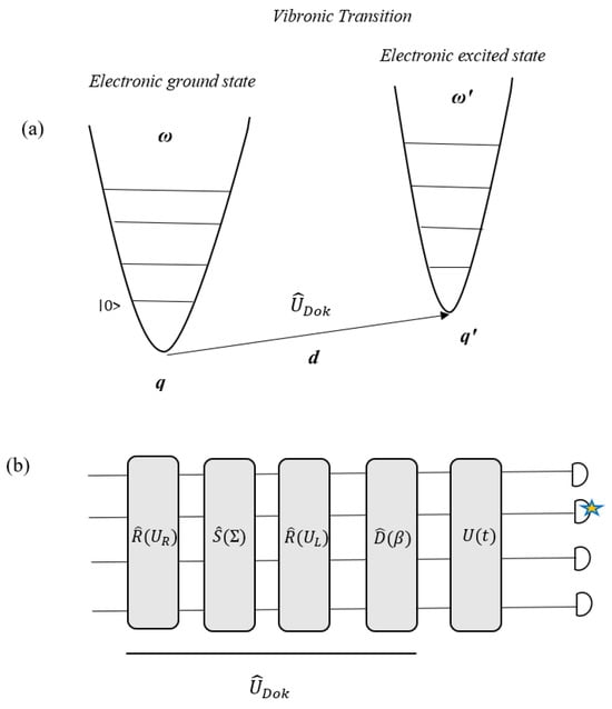
Figure 15. (a) Schematic representation of a vibronic transition. (b) Implementation of Doktorov operator operations in a GBS device [6,112]. (Reproduced with permission from [Bromley, T.R.; Arrazola, J.M.; Jahangiri, S.; Izaac, J.; Quesada, N.; Gran, A.D.; Schuld, M.; Swinarton, J.; Zabaneh, Z.; Kil-loran, N. Applications of near-term photonic quantum computers: Software and algorithms. arXiv 2019, arXiv: 1912.07634]).

To obtain the other matrices of the Doktorov operator, $U_L$, $U_R$, and $\mathsf{\Sigma }$, the diagonal matrices $\mathsf{\Omega }$ and $\acute{\mathsf{\Omega }}$ must be found via the ground and excited state frequencies as follows:

$$\mathsf{\Omega }=diag\left(\sqrt{{\omega }_1} ,\dots ,\sqrt{{\omega }_M} \right)$$

(36)

$$\acute{\Omega }=diag\left(\sqrt{\acute{{\omega }_1}} ,\dots ,\sqrt{\acute{{\omega }_M}} \right)$$

(37)

Then, matrix J can be obtained from the diagonal matrices ${\Omega }^{-1}$, $\acute{\mathsf{\Omega }}$ and $U_D$ as

$$J=\acute{\Omega }{U}_D{\mathsf{\Omega }}^{-1}$$

(38)

Finally, the matrices $U_L$, $U_R$, and $\mathsf{\Sigma }$, are computable from the singular value decomposition of $J=U_L\mathsf{\Sigma }{U}_R$.

Also, the displacement vector $\beta$ in the Doktorov operator can be calculated by the following equation ($\hslash$ is the reduced Planck constant):

$$\beta ={\hslash }^{-1/2}\acute{\mathsf{\Omega }}d/\sqrt{2}$$

(39)

After the determination of the ${\widehat{U}}_{Dok}$, by all the existing elements $\mathsf{\Omega }$, $\acute{\Omega }$, $U_D$, and d, the excitation of vibrational modes through a vibrational transition can be determined using the GBS quantum algorithm [112].

So, the steps of the GBS algorithm to simulate molecular vibrational excitations in a vibronic transition are as follows:

1.

The input chemical data $\mathsf{\Omega }$, $\acute{\Omega }$, $U_D$, and d can be used to calculate the GBS parameters $U_L$, $U_R$, $\mathsf{\Sigma }$, and $\beta$.

2.

The GBS device has been used to make the Gaussian state $|\psi ⟩=$${\widehat{U}}_{Dok}|{\psi }_i⟩$, ($|{\psi }_i⟩$ is an initial Gaussian state) with covariance matrix V and vector of means $\alpha$.

3.

The simulation of the vibrational quantum dynamics in the localized modes can be performed by the implementation of the unitary transformation $U\left(t\right)=\widehat{R}\left(U_l\right)e^{-i\widehat{H}t/\hslash }$. ($\widehat{H}$ is the Hamiltonian related to the harmonic normal modes, t is time. $\widehat{R}\left(U_l\right)$ signifies an interferometer configured with a unitary matrix $U_l$, in which $U_l$ transforms the molecular normal modes into a collection of spatially localized vibrational modes.

4.

Generate samples by calculating the output state based on the photon number.

5.

The above steps can be repeated appropriately several times to find the preferred statistics about the vibrational excitation distributions.

Only some of the vibrational modes are important, and it is enough for sampling from their marginal distribution. Since the ultimate state of the vibrational modes is Gaussian, Gaussian states and the reduced states are quantified by their vector of means α and covariance matrix V [77]. When the aim is to sample from the marginal distribution of the first k modes of an M-mode initial state, for example, modes i (i = 1,2,…,k) of an M-mode system, the reduced covariance matrix V_k (2k × 2k) can be found by choosing the (i, i + M) rows and columns of the main covariance matrix V. Also, the reduced vector of means, α_k, can be created by selecting only the first k elements of the main vector (Figure 16). Then, these matrices can be encoded into a GBS machine to sample from the preferred marginal distribution [6,112].

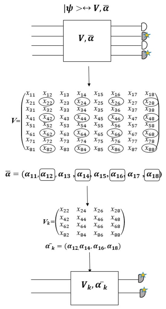
Figure 16. One example of a sampling algorithm from the marginal distribution of modes 2 and 4 of a 4-mode system to obtain vibrational modes [112]. (Reproduced with permission from [Jahangiri, S.; Arrazola, J.M.; Quesada, N.; Delgado, A. Quantum algorithm for simulating molecular vibrational excitations. arXiv 2020, arXiv: 2006.13339]).

Because of the similarity between the next equation (Equation (40)), which indicates the observing probability of an output state $\left|m\right.⟩$ from an initial state $\left|n\right.⟩$ in a programmed GBS with ${\widehat{U}}_{Dok}$, and Equation (29), the chemical data describing a vibronic transition can be encoded into a GBS, and then sampling from this distribution can be performed to specify the statistics of the obtained vibrational excitations.

$$\mathrm{Pr}\left(m,n\right)={\left|⟨m\left|{\widehat{U}}_{Dok}\right|n⟩\right|}^2$$

(40)

The probability of observing an output state in a GBS setting can be computed by [146]

$$\mathrm{Pr}\left(m,n\right)={\displaystyle \frac{lhaf(\acute{{\mathcal{A}}_{m,n})}}{\mathcal{N}}}$$

(41)

where ${\acute{\mathcal{A}}}_{m,n}$ is a matrix obtained by the covariance matrix and displacement vector of the Gaussian state organized by the GBS machine and via the distribution of ground and excited vibrational quanta (m, n), where lhaf(.) [82] is a loop hafnian matrix function and $\mathcal{N}$ is a normalization constant [112].

In Ref. [112], a quantum algorithm based on GBS is used to predict the vibrational excitation distribution of pyrrole and butane during a vibronic transition. The marginal distributions of the normal modes of pyrrole computed from the GBS samples (Figures 3 and 4 in Ref. [112].) show similar excited normal mode frequencies (1518.1 cm⁻¹, 1080.5 cm⁻¹, and 882.3 cm⁻¹) to the experimental results. Also, quantum-inspired classical methods are implemented for specific cases where excitations are important only in a few modes. However, the required time to sample with these algorithms is very long when the number of modes is large. So, GBS can be useful when large numbers of modes should be simulated. The achieved results show that the vibrational excitations obtained by GBS can explain the experimental outcomes.

7. Perspectives

The reported graph-based problems [10,107] involve relatively large and complex graphs, with more than eight vertices, which have been solved with GBS using the Strawberry Fields simulator.

One of the goals of our work is to define small graph-based problems, especially problems related to molecular docking, that involve graphs with four or eight vertices that can be solved by four or eight optical mode-integrated photonic quantum computers based on GBS or Strawberry Fields.

Hence, the searching and finding of graph-based problems, which will be expressed as small graphs (four or eight vertices) that can be solved by four or eight optical mode photonic quantum computers, should be investigated.

However, the molecular docking problems that have been solved with QAOA [25] have been defined as 6-, 8-, and 12-vertex graphs, which can be considered as problems that can be solved by photonic quantum computers with 6, 8, and 12 vertices based on Gaussian Boson Sampling.

8. Conclusions

In recent years, quantum computers have made significant progress in solving specific computational problems due to their quantum mechanical properties, such as superposition and entanglement, compared with classical computing. NISQ computers, which have been considered in this study, can only be used to solve particular problems. So, it is very important to identify the problems that can be solved by NISQ systems.

Nowadays, photonic quantum computers have attracted much attention compared with other technologies, and various applications have been reported for them.

Xanadu is one of the few well-known companies active in the field of developing integrated photonic quantum computer hardware, as well as developing software packages and photonic quantum computing simulators. By introducing the X8 quantum chip based on integrated photonic technology and the important and widely used computing platforms PennyLane and Strawberry Fields, it has taken a very important step towards solving some fundamental problems, including chemistry problems. Gaussian Boson Sampling (GBS), an algorithm available in the Xanadu cloud, can solve some specific problems. In this paper, after a review of BS and GBS, the relationship between GBS and graph theory, as well as how to encode graphs in Gaussian Boson Sampling, and also graphs that can be embedded in X8, is explained. Also, some applications of the Strawberry Fields platform and how to use Gaussian Boson Sampling to solve problems, especially those based on graph theory, such as molecular docking, have been investigated.

The search and discovery of problems based on graphs, which will be expressed as four- or eight-vertex graphs that can be solved by four or eight optical mode photonic quantum computers based on GBS, is one of the main aims of these studies in the future.

References

- Hassija, V.; Chamola, V.; Goyal, A.; Kanhere, S.S.; Guizani, N. Forthcoming applications of quantum computing: Peeking into the future. IET Quantum Commun. 2020, 1, 35–41. [Google Scholar] [CrossRef]
- Vedral, V.; Plenio, M.B. Basics of quantum computation. Prog. Quantum Electron. 1998, 22, 1–39. [Google Scholar] [CrossRef]
- Kockum, A.F.; Soro, A.; García-Álvarez, L.; Vikstål, P.; Douce, T.; Johansson, G.; Ferrini, G. Lecture notes on quantum computing. arXiv 2023, arXiv:2311.08445. [Google Scholar]
- Manin, Y.I. Classical computing, quantum computing, and Shor’s factoring algorithm. Asterisque-Soc. Math. De Fr. 2000, 266, 375–404. [Google Scholar]
- Ladd, T.D.; Jelezko, F.; Laflamme, R.; Nakamura, Y.; Monroe, C.; O’Brien, J.L. Quantum computers. Nature 2010, 464, 45–53. [Google Scholar] [CrossRef]
- Bromley, T.R.; Arrazola, J.M.; Jahangiri, S.; Izaac, J.; Quesada, N.; Gran, A.D.; Schuld, M.; Swinarton, J.; Zabaneh, Z.; Killoran, N. Applications of near-term photonic quantum computers: Software and algorithms. arXiv 2019, arXiv:1912.07634. [Google Scholar] [CrossRef]
- Paudel, H.P.; Syamlal, M.; Crawford, S.E.; Lee, Y.-L.; Shugayev, R.A.; Lu, P.; Ohodnicki, P.R.; Mollot, D.; Duan, Y. Quantum computing and simulations for energy applications: Review and perspective. ACS Eng. Au 2022, 2, 151–196. [Google Scholar] [CrossRef]
- Feynman, R.P. Simulating physics with computers. Int. J. Theor. Phys. 1982, 21, 467–488. [Google Scholar] [CrossRef]
- Nielsen, M.A.; Chuang, I.L. Quantum Computation and Quantum Information; Cambridge University Press: Cambridge, UK, 2001; Volume 2. [Google Scholar]
- Banchi, L.; Fingerhuth, M.; Babej, T.; Ing, C.; Arrazola, J.M. Molecular docking with Gaussian boson sampling. arXiv 2019, arXiv:1902.00462v1. [Google Scholar] [CrossRef]
- Aaronson, S. Quantum Computing Since Democritus; Cambridge University Press: Cambridge, UK, 2013. [Google Scholar]
- Santagati, R.; Aspuru-Guzik, A.; Babbush, R.; Degroote, M.; González, L.; Kyoseva, E.; Moll, N.; Oppel, M.; Parrish, R.M.; Rubin, N.C.; et al. Drug design on quantum computers. Nat. Phys. 2024, 20, 549–557. [Google Scholar] [CrossRef]
- Romero, J.; Milburn, G. Photonic Quantum Computing. arXiv 2024, arXiv:2404.03367. [Google Scholar]
- Liu, H.; Low, G.H.; Steiger, D.S.; Häner, T.; Reiher, M.; Troyer, M. Prospects of quantum computing for molecular sciences. Mater. Theory 2022, 6, 11. [Google Scholar] [CrossRef]
- Shor, P.W. Algorithms for quantum computation: Discrete logarithms and factoring. In Proceedings of the 35th Annual Symposium on Foundations of Computer Science, Washington, DC, USA, 20–22 November 1994; pp. 124–134. [Google Scholar]
- Mulligan, V.K.; Melo, H.; Merritt, H.I.; Slocum, S.; Weitzner, B.D.; Watkins, A.M.; Renfrew, P.D.; Pelissier, C.; Arora, P.S.; Bonneau, R. Designing peptides on a quantum computer. BioRxiv 2019, 752485. [Google Scholar] [CrossRef]
- Robert, A.; Barkoutsos, P.K.; Woerner, S.; Tavernelli, I. Resource-efficient quantum algorithm for protein folding. Npj Quantum Inf. 2021, 7, 38. [Google Scholar] [CrossRef]
- Fox, D.M.; MacDermaid, C.M.; Schreij, A.M.; Zwierzyna, M.; Walker, R.C. RNA folding using quantum computers. PLoS Comput. Biol. 2022, 18, e1010032. [Google Scholar] [CrossRef] [PubMed]
- GAO-22-104422; Quantum Computing and Communications. Government Accountability Office: Washington, DC, USA, 2021.
- Preskill, J. Quantum computing in the NISQ era and beyond. Quantum 2018, 2, 79. [Google Scholar] [CrossRef]
- Katabarwa, A.; Gratsea, K.; Caesura, A.; Johnson, P.D. Early fault-tolerant quantum computing. PRX Quantum 2024, 5, 020101. [Google Scholar] [CrossRef]
- Gidney, C.; Ekerå, M. How to factor 2048 bit RSA integers in 8 h using 20 million noisy qubits. Quantum 2021, 5, 433. [Google Scholar] [CrossRef]
- Lloyd, S. Universal quantum simulators. Science 1996, 273, 1073–1078. [Google Scholar] [CrossRef]
- Berry, D.W.; Childs, A.M.; Kothari, R. Hamiltonian Simulation with Nearly Optimal Dependence on all Parameters. In Proceedings of the IEEE 56th Annual Symposium on Foundations of Computer Science (FOCS), Berkeley, CA, USA, 17–20 October 2015. [Google Scholar]
- Ding, Q.M.; Huang, Y.M.; Yuan, X. Molecular docking via quantum approximate optimization algorithm. Phys. Rev. Appl. 2024, 21, 034036. [Google Scholar] [CrossRef]
- Acín, A.; Bloch, I.; Buhrman, H.; Calarco, T.; Eichler, C.; Eisert, J.; Esteve, D.; Gisin, N.; Glaser, S.J.; Jelezko, F.; et al. The quantum technologies roadmap: A European community view. New J. Phys. 2018, 20, 080201. [Google Scholar] [CrossRef]
- Bharti, K.; Cervera-Lierta, A.; Kyaw, T.H.; Haug, T.; Alperin-Lea, S.; Anand, A.; Degroote, M.; Heimonen, H.; Kottmann, J.S.; Menke, T.; et al. Noisy intermediate-scale quantum algorithms. Rev. Mod. Phys. 2022, 94, 015004. [Google Scholar] [CrossRef]
- Kadowaki, T.; Nishimori, H. Quantum annealing in the transverse Ising model. Phys. Rev. E 1998, 58, 5355–5363. [Google Scholar] [CrossRef]
- Aaronson, S.; Arkhipov, A. The computational complexity of linear optics. In Proceedings of the Forty-Third Annual ACM Symposium on Theory of Computing, San Jose, CA, USA, 6–8 June 2011; pp. 333–342. [Google Scholar]
- Georgescu, I.M.; Ashhab, S.; Nori, F. Quantum simulation. Rev. Mod. Phys. 2014, 86, 153–185. [Google Scholar] [CrossRef]
- O’brien, J.L.; Furusawa, A.; Vučković, J. Photonic quantum technologies. Nat. Photonics 2009, 3, 687–695. [Google Scholar] [CrossRef]
- Knill, E.; Laflamme, R.; Milburn, G.J. A scheme for efficient quantum computation with linear optics. Nature 2001, 409, 46–52. [Google Scholar] [CrossRef]
- Dellios, A.S.; Reid, M.D.; Drummond, P.D. Simulating Gaussian boson sampling quantum computers. AAPPS Bull. 2023, 33, 31. [Google Scholar] [CrossRef]
- McMahon, P.L.; Marandi, A.; Haribara, Y.; Hamerly, R.; Langrock, C.; Tamate, S.; Inagaki, T.; Takesue, H.; Utsunomiya, S.; Aihara, K.; et al. A fully programmable 100-spin coherent Ising machine with all-to-all connections. Science 2016, 354, 614–617. [Google Scholar] [CrossRef]
- Lloyd, S.; Braunstein, S.L. Quantum computation over continuous variables. Phys. Rev. Lett. 1999, 82, 1784. [Google Scholar] [CrossRef]
- Killoran, N.; Izaac, J.; Quesada, N.; Bergholm, V.; Amy, M.; Weedbrook, C. Strawberry fields: A software platform for photonic quantum computing. Quantum 2019, 3, 129. [Google Scholar] [CrossRef]
- Zhong, H.-S.; Wang, H.; Deng, Y.-H.; Chen, M.-C.; Peng, L.-C.; Luo, Y.-H.; Qin, J.; Wu, D.; Ding, X.; Hu, Y.; et al. Quantum computational advantage using photons. Science 2020, 370, 1460–1463. [Google Scholar] [CrossRef] [PubMed]
- Zhong, H.-S.; Deng, Y.-H.; Qin, J.; Wang, H.; Chen, M.-C.; Peng, L.-C.; Luo, Y.-H.; Wu, D.; Gong, S.-Q.; Su, H.; et al. Phase-programmable gaussian boson sampling using stimulated squeezed light. Phys. Rev. Lett. 2021, 127, 180502. [Google Scholar] [CrossRef] [PubMed]
- Madsen, L.S.; Laudenbach, F.; Askarani, M.F.; Rortais, F.; Vincent, T.; Bulmer, J.F.F.; Miatto, F.M.; Neuhaus, L.; Helt, L.G.; Collins, M.J.; et al. Quantum computational advantage with a programmable photonic processor. Nature 2022, 606, 75–81. [Google Scholar] [CrossRef] [PubMed]
- Liao, S.-K.; Cai, W.-Q.; Liu, W.-Y.; Zhang, L.; Li, Y.; Ren, J.-G.; Yin, J.; Shen, Q.; Cao, Y.; Li, Z.-P.; et al. Satellite-to-ground quantum key distribution. Nature 2017, 549, 43–47. [Google Scholar] [CrossRef]
- Ren, J.-G.; Xu, P.; Yong, H.-L.; Zhang, L.; Liao, S.-K.; Yin, J.; Liu, W.-Y.; Cai, W.-Q.; Yang, M.; Li, L.; et al. Ground-to-satellite quantum teleportation. Nature 2017, 549, 70–73. [Google Scholar] [CrossRef]
- Chen, Y.-A.; Zhang, Q.; Chen, T.-Y.; Cai, W.-Q.; Liao, S.-K.; Zhang, J.; Chen, K.; Yin, J.; Ren, J.-G.; Chen, Z.; et al. An integrated space-to-ground quantum communication network over 4600 kilometres. Nature 2021, 589, 214–219. [Google Scholar] [CrossRef]
- Steinbrecher, G.R.; Olson, J.P.; Englund, D.; Carolan, J. Quantum optical neural networks. Npj Quantum Inf. 2019, 5, 60. [Google Scholar] [CrossRef]
- Shen, Y.; Harris, N.C.; Skirlo, S.; Prabhu, M.; Baehr-Jones, T.; Hochberg, M.; Sun, X.; Zhao, S.; Larochelle, H.; Englund, D.; et al. Deep learning with coherent nanophotonic circuits. Nat. Photonics 2017, 11, 441–446. [Google Scholar] [CrossRef]
- Stipcevic, M. Quantum random number generators and their applications in cryptography. In Advanced Photon Counting Techniques VI; SPIE: Paris, France, 2012; Volume 8375, pp. 20–34. [Google Scholar]
- Paraiso, T.K.; Roger, T.; Marangon, D.G.; De Marco, I.; Sanzaro, M.; Woodward, R.I.; Dynes, J.F.; Yuan, Z.; Shields, A.J. A photonic integrated quantum secure communication system. Nat. Photonics 2021, 15, 850–856. [Google Scholar] [CrossRef]
- Sparrow, C.; Martín-López, E.; Maraviglia, N.; Neville, A.; Harrold, C.; Carolan, J.; Joglekar, Y.N.; Hashimoto, T.; Matsuda, N.; O’bRien, J.L.; et al. Simulating the vibrational quantum dynamics of molecules using photonics. Nature 2018, 557, 660–667. [Google Scholar] [CrossRef]
- Zini, M.S.; Delgado, A.; dos Reis, R.; Casares, P.A.M.; Mueller, J.E.; Voigt, A.C.; Arrazola, J.M. Quantum simulation of battery materials using ionic pseudopotentials. Quantum 2023, 7, 1049. [Google Scholar] [CrossRef]
- Ceroni, J.; Stetina, T.F.; Kieferova, M.; Marrero, C.O.; Arrazola, J.M.; Wiebe, N. Generating approximate ground states of molecules using quantum machine learning. arXiv 2022, arXiv:2210.05489. [Google Scholar]
- Castaldo, D.; Jahangiri, S.; Delgado, A.; Corni, S. Quantum simulation of molecules in solution. J. Chem. Theory Comput. 2022, 18, 7457–7469. [Google Scholar] [CrossRef] [PubMed]
- Delgado, A.; Arrazola, J.M.; Jahangiri, S.; Niu, Z.; Izaac, J.; Roberts, C.; Killoran, N. Variational quantum algorithm for molecular geometry optimization. Phys. Rev. A 2021, 104, 052402. [Google Scholar] [CrossRef]
- Pelucchi, E.; Fagas, G.; Aharonovich, I.; Englund, D.; Figueroa, E.; Gong, Q.; Hannes, H.; Liu, J.; Lu, C.-Y.; Matsuda, N.; et al. The potential and global outlook of integrated photonics for quantum technologies. Nat. Rev. Phys. 2022, 4, 194–208. [Google Scholar] [CrossRef]
- Deng, Y.-H.; Gu, Y.-C.; Liu, H.-L.; Gong, S.-Q.; Su, H.; Zhang, Z.-J.; Tang, H.-Y.; Jia, M.-H.; Xu, J.-M.; Chen, M.-C.; et al. Gaussian boson sampling with pseudo-photon-number-resolving detectors and quantum computational advantage. Phys. Rev. Lett. 2023, 131, 150601. [Google Scholar] [CrossRef]
- ORCA Computing. Available online: https://www.orcacomputing.com (accessed on 26 November 2025).
- Psiquantum. PsiQuantum Closes $450 Million Funding Round to Build the World’s First Commercially Viable Quantum Computer. Psiquantum, 22 07 2021. Available online: https://psiquantum.com/news/psiquantum-closes-450-million-funding-round-to-build-the-worlds-first-commercially-viable-quantum-computer (accessed on 26 November 2025).
- Quandela Announces a European Quantum Cloud Service. Available online: https://quantumcomputingreport.com/quandela-announces-a-european-quantum-cloud-service/ (accessed on 26 November 2025).
- Delivering Quantum Powerful and Deployable at Scale. Available online: https://www.quixquantum.com/ (accessed on 26 November 2025).
- On-Chip Error-Resistant Photonic Qubits. Available online: https://www.xanadu.ai (accessed on 26 November 2025).
- Bergholm, V.; Izaac, J.; Schuld, M.; Gogolin, C.; Ahmed, S.; Ajith, V.; Alam, M.S.; Alonso-Linaje, G.; AkashNarayanan, B.; Ali Asadi, A.; et al. Pennylane: Automatic differentiation of hybrid quantum-classical computations. arXiv 2018, arXiv:1811.04968. [Google Scholar]
- Arrazola, J.M.; Bergholm, V.; Brádler, K.; Bromley, T.R.; Collins, M.J.; Dhand, I.; Fumagalli, A.; Gerrits, T.; Goussev, A.; Helt, L.G.; et al. Quantum circuits with many photons on a programmable nanophotonic chip. arXiv 2021, arXiv:2103.02109. [Google Scholar] [CrossRef]
- Quantum Algorithms on the Xanadu Quantum Cloud. Available online: https://strawberryfields.ai/photonics/demos/tutorial_X8_demos.html (accessed on 26 November 2025).
- Larsen, M.V.; Bourassa, J.E.; Kocsis, S.; Tasker, J.F.; Chadwick, R.S.; González-Arciniegas, C.; Hastrup, J.; Lopetegui-González, C.E.; Miatto, F.M.; Motamedi, A. Integrated photonic source of Gottesman–Kitaev–Preskill qubits. Nature 2025, 642, 1–51. [Google Scholar] [CrossRef]
- Rad, H.A.; Ainsworth, T.; Alexander, R.N.; Altieri, B.; Askarani, M.F.; Baby, R.; Banchi, L.; Baragiola, B.Q.; Bourassa, J.E.; Chadwick, R.S.; et al. Scaling and networking a modular photonic quantum computer. Nature 2025, 638, 912–919. [Google Scholar] [CrossRef]
- Hamilton, C.S.; Kruse, R.; Sansoni, L.; Barkhofen, S.; Silberhorn, C.; Jex, I. Gaussian boson sampling. Phys. Rev. Lett. 2017, 119, 170501. [Google Scholar] [CrossRef]
- Kruse, R.; Hamilton, C.S.; Sansoni, L.; Barkhofen, S.; Silberhorn, C.; Jex, I. A detailed study of Gaussian boson sampling. Phys. Rev. A 2019, 100, 032326. [Google Scholar] [CrossRef]
- Quesada, N.; Arrazola, J.M. Exact simulation of Gaussian boson sampling in polynomial space and exponential time. Phys. Rev. Res. 2020, 2, 023005. [Google Scholar] [CrossRef]
- Arrazola, J.M.; Bromley, T.R.; Rebentrost, P. Quantum approximate optimization with Gaussian boson sampling. Phys. Rev. A 2018, 98, 012322. [Google Scholar] [CrossRef]
- Sempere-Llagostera, S.; Patel, R.B.; Walmsley, I.A.; Kolthammer, W.S. Experimentally finding dense subgraphs using a time-bin encoded Gaussian boson sampling device. Phys. Rev. X 2022, 12, 031045. [Google Scholar] [CrossRef]
- Liu, Y.; Wu, J.; Yi, X. Quantum Boson-Sampling Machine. In Proceedings of the International Conference on Natural Computation (ICNC), Zhangjiajie, China, 15–17 August 2015. [Google Scholar]
- Brod, D.J.; Galvão, E.F.; Crespi, A.; Osellame, R.; Spagnolo, N.; Sciarrino, F. Photonic implementation of boson sampling: A review. Adv. Photonics 2019, 1, 034001. [Google Scholar]
- Li, Y.; Gan, L.; Chen, M.; Chen, Y.; Lu, H.; Lu, C.; Pan, J.; Fu, H.; Yang, G. Benchmarking 50-photon gaussian boson sampling on the sunway TaihuLight. IEEE Trans. Parallel Distrib. Syst. 2021, 33, 1357–1372. [Google Scholar] [CrossRef]
- Gard, B.T.; Motes, K.R.; Olson, J.P.; Rohde, P.P.; Dowling, J.P. An introduction to boson-sampling. In From Atomic to Mesoscale: The Role of Quantum Coherence in Systems of Various Complexities; World Scientific Publishing: Singapore, 2015; pp. 167–192. [Google Scholar]
- Ryser, H.J. Combinatorial Mathematics; American Mathematical Soc.: Providence, RI, USA, 1963. [Google Scholar]
- Grier, D.; Brod, D.J.; Arrazola, J.M.; de Andrade Alonso, M.B.; Quesada, N. The complexity of bipartite Gaussian boson sampling. arXiv 2021, arXiv:2110.06964. [Google Scholar] [CrossRef]
- Weedbrook, C.; Pirandola, S. Gaussian quantum information. Rev. Mod. Phys. 2012, 84, 621–669. [Google Scholar] [CrossRef]
- Serafini, A. Quantum Continuous Variables: A Primer of Theoretical Methods; CRC Press: Boca Raton, FL, USA, 2017. [Google Scholar]
- Picinbono, B. Second-order complex random vectors and normal distributions. IEEE Trans. Signal Process. 1996, 44, 2637–2640. [Google Scholar] [CrossRef]
- Ferraro, A.; Olivares, S.; Paris, M.G. Gaussian states in continuous variable quantum information. arXiv 2005, arXiv:quant-ph/0503237. [Google Scholar] [CrossRef]
- Simon, R.; Mukunda, N.; Dutta, B. Quantum-noise matrix for multimode systems: U (n) invariance, squeezing, and normal forms. Phys. Rev. A 1994, 49, 1567. [Google Scholar] [CrossRef] [PubMed]
- Stanev, D.; Giordani, T.; Spagnolo, N.; Sciarrino, F. Testing of on-cloud Gaussian Boson Sampler “Borealis” via graph theory. arXiv 2023, arXiv:2306.12120. [Google Scholar] [CrossRef]
- Giordani, T.; Mannucci, V.; Spagnolo, N.; Fumero, M.; Rampini, A.; Rodolà, E.; Sciarrino, F. Certification of Gaussian Boson Sampling via graph theory. arXiv 2022, arXiv:2202.07711. [Google Scholar] [CrossRef]
- Björklund, A.; Gupt, B.; Quesada, N. A faster hafnian formula for complex matrices and its benchmarking on a supercomputer. J. Exp. Algorithmics (JEA) 2019, 24, 1–17. [Google Scholar] [CrossRef]
- Schuld, M.; Brádler, K.; Israel, R.; Su, D.; Gupt, B. Measuring the similarity of graphs with a Gaussian boson sampler. Phys. Rev. A 2020, 101, 032314. [Google Scholar] [CrossRef]
- Quesada, N.; Arrazola, J.M.; Killoran, N. Gaussian boson sampling using threshold detectors. Phys. Rev. A 2018, 98, 062322. [Google Scholar] [CrossRef]
- Jahangiri, S.; Arrazola, J.M.; Quesada, N.; Killoran, N. Point processes with Gaussian boson sampling. Phys. Rev. E 2020, 101, 022134. [Google Scholar] [CrossRef]
- Rabani, Y. (Ed.) In Proceedings of the Twenty-Third Annual ACM-SIAM Symposium on Discrete Algorithms, Society for Industrial and Applied Mathematics, Kyoto, Japan, 17–19 January 2012.
- Deshpande, A.; Mehta, A.; Vincent, T.; Quesada, N.; Hinsche, M.; Ioannou, M.; Madsen, L.; Lavoie, J.; Qi, H.; Eisert, J.; et al. Quantum computational advantage via high-dimensional Gaussian boson sampling. Sci. Adv. 2022, 8, eabi7894. [Google Scholar] [CrossRef]
- Arrazola, J.M.; Bromley, T.R. Using Gaussian boson sampling to find dense subgraphs. Phys. Rev. Lett. 2018, 121, 030503. [Google Scholar] [CrossRef]
- Brádler, K.; Friedland, S.; Izaac, J.; Killoran, N.; Su, D. Graph isomorphism and Gaussian boson sampling. Spec. Matrices 2021, 9, 166–196. [Google Scholar] [CrossRef]
- Deng, Y.-H.; Gong, S.-Q.; Gu, Y.-C.; Zhang, Z.-J.; Liu, H.-L.; Su, H.; Tang, H.-Y.; Xu, J.-M.; Jia, M.-H.; Chen, M.-C.; et al. Solving graph problems using gaussian boson sampling. Phys. Rev. Lett. 2023, 130, 190601. [Google Scholar] [CrossRef]
- Zhu, H.; Chen, H.; Li, S.; Chen, T.; Li, Y.; Luo, X.; Gao, F.; Li, Q.; Zhou, L.; Karim, M.F.; et al. A dynamically programmable quantum photonic microprocessor for graph computation. Laser Photonics Rev. 2024, 18, 2300304. [Google Scholar] [CrossRef]
- Oh, C.; Fefferman, B.; Jiang, L.; Quesada, N. Quantum-inspired classical algorithm for graph problems by Gaussian boson sampling. arXiv 2023, arXiv:2302.00536. [Google Scholar] [CrossRef]
- Brádler, K.; Dallaire-Demers, P.L.; Rebentrost, P.; Su, D.; Weedbrook, C. Gaussian boson sampling for perfect matchings of arbitrary graphs. Phys. Rev. A 2018, 98, 032310. [Google Scholar] [CrossRef]
- Eppstein, D. The graphs of stably matchable pairs. In Graph—Theoretic Concepts in Computer Science, Proceedings of the 47th International Workshop, Warsaw, Poland, 6–8 May 2021; Springer: Cham, Switzerland, 2021. [Google Scholar]
- Oh, C.; Lim, Y.; Fefferman, B.; Jiang, L. Classical simulation of boson sampling based on graph structure. Phys. Rev. Lett. 2022, 128, 190501. [Google Scholar] [CrossRef]
- Horn, R.A.; Johnson, C.R. Matrix Analysis; Cambridge University Press: Cambridge, UK, 2012. [Google Scholar]
- Cariolaro, G.; Pierobon, G. Bloch-Messiah reduction of Gaussian unitaries by Takagi factorization. Phys. Rev. A 2016, 94, 062109. [Google Scholar] [CrossRef]
- Kumar, R.; Raghavan, P.; Rajagopalan, S.; Tomkins, A. Trawling the web for emerging cyber-communities. Comput. Netw. 1999, 31, 1481–1493. [Google Scholar] [CrossRef]
- Arora, S.; Barak, B.; Brunnermeier, M.; Ge, R. Computational complexity and information asymmetry in financial products. Commun. ACM 2011, 54, 101–107. [Google Scholar] [CrossRef]
- Angel, A.; Koudas, N.; Sarkas, N.; Srivastava, D. Dense subgraph maintenance under streaming edge weight updates for real-time story identification. arXiv 2012, arXiv:1203.0060. [Google Scholar] [CrossRef]
- Fratkin, E.; Naughton, B.T.; Brutlag, D.L.; Batzoglou, S. MotifCut: Regulatory motifs finding with maximum density subgraphs. Bioinformatics 2006, 22, e150–e157. [Google Scholar] [CrossRef]
- Balasundaram, B.; Butenko, S.; Hicks, I.V. Clique relaxations in social network analysis: The maximum k-plex problem. Oper. Res. 2011, 59, 133–142. [Google Scholar] [CrossRef]
- Gómez Ravetti, M.; Moscato, P. Identification of a 5-protein biomarker molecular signature for predicting Alzheimer’s disease. PLoS ONE 2008, 3, e3111. [Google Scholar] [CrossRef] [PubMed]
- Dorndorf, U.; Jaehn, F.; Pesch, E. Modelling robust flight-gate scheduling as a clique partitioning problem. Transp. Sci. 2008, 42, 292–301. [Google Scholar] [CrossRef]
- Jain, K.; Padhye, J.; Padmanabhan, V.N.; Qiu, L. Impact of interference on multi-hop wireless network performance. In Proceedings of the 9th Annual International Conference on Mobile Computing and Networking, San Diego, CA, USA, 14–19 September 2003. [Google Scholar]
- Boginski, V.; Butenko, S.; Pardalos, P.M. Mining market data: A network approach. Comput. Oper. Res. 2006, 33, 3171–3184. [Google Scholar] [CrossRef]
- Yu, S.; Zhong, Z.-P.; Fang, Y.; Patel, R.B.; Li, Q.-P.; Liu, W.; Li, Z.; Xu, L.; Sagona-Stophel, S.; Mer, E.; et al. A universal programmable gaussian boson sampler for drug discovery. arXiv 2022, arXiv:2210.14877. [Google Scholar] [CrossRef]
- Pierre, E.; Nowak, M. Towards graph classification with Gaussian Boson Sampling by embedding graphs on the X8 photonic chip. arXiv 2021, arXiv:2109.12863. [Google Scholar] [CrossRef]
- Executing Programs on X8 Devices. Available online: https://strawberryfields.ai/photonics/demos/tutorial_X8.html (accessed on 26 November 2025).
- Applications. Available online: https://strawberryfields.ai/photonics/applications.html (accessed on 26 November 2025).
- Hoch, F.; Caruccio, E.; Rodari, G.; Francalanci, T.; Suprano, A.; Giordani, T.; Carvacho, G.; Spagnolo, N.; Koudia, S.; Proietti, M.; et al. Quantum machine learning with Adaptive Boson Sampling via post-selection. Nat. Commun. 2025, 16, 902. [Google Scholar] [CrossRef]
- Jahangiri, S.; Arrazola, J.M.; Quesada, N.; Delgado, A. Quantum algorithm for simulating molecular vibrational excitations. arXiv 2020, arXiv:2006.13339. [Google Scholar] [CrossRef]
- Li, Y.; Zhu, H.; Luo, W.; Cai, H.; Karim, M.F.; Luo, X.; Gao, F.; Wu, X.; Zhou, X.; Song, Q.; et al. Realizing ultrahigh capacity quantum superdense coding on quantum photonic chip. Npj Quantum Inf. 2025, 11, 49. [Google Scholar] [CrossRef]
- Sawaya, N.P.; Huh, J. Quantum algorithm for calculating molecular vibronic spectra. J. Phys. Chem. Lett. 2019, 10, 3586–3591. [Google Scholar] [CrossRef]
- Huh, J.; Guerreschi, G.G.; Peropadre, B.; McClean, J.R.; Aspuru-Guzik, A. Boson sampling for molecular vibronic spectra. Nat. Photonics 2015, 9, 615–620. [Google Scholar] [CrossRef]
- Lyu, N.; Bergold, P.; Soley, M.B.; Wang, C.; Batista, V.S. Holographic Gaussian Boson Sampling with Matrix Product States on 3D cQED Processors. J. Chem. Theory Comput. 2024, 20, 6402–6413. [Google Scholar] [CrossRef] [PubMed]
- Chandarana, P.; Hegade, N.N.; Montalban, I.; Solano, E.; Chen, X. Digitized counterdiabatic quantum algorithm for protein folding. Phys. Rev. Appl. 2023, 20, 014024. [Google Scholar] [CrossRef]
- Perdomo, A.; Truncik, C.; Tubert-Brohman, I.; Rose, G.; Aspuru-Guzik, A. Construction of model Hamiltonians for adiabatic quantum computation and its application to finding low-energy conformations of lattice protein models. Phys. Rev. A—At. Mol. Opt. Phys. 2008, 78, 012320. [Google Scholar] [CrossRef]
- Perdomo-Ortiz, A.; Dickson, N.; Drew-Brook, M.; Rose, G.; Aspuru-Guzik, A. Finding low-energy conformations of lattice protein models by quantum annealing. Sci. Rep. 2012, 2, 1–7. [Google Scholar] [CrossRef]
- Irbäck, A.; Knuthson, L.; Mohanty, S.; Peterson, C. Folding lattice proteins with quantum annealing. Phys. Rev. Res. 2022, 4, 043013. [Google Scholar] [CrossRef]
- Fingerhuth, M.; Babej, T. A quantum alternating operator ansatz with hard and soft constraints for lattice protein folding. arXiv 2018, arXiv:1810.13411. [Google Scholar] [CrossRef]
- Babej, T.; Fingerhuth, M. Coarse-grained lattice protein folding on a quantum annealer. arXiv 2018, arXiv:1811.00713. [Google Scholar] [CrossRef]
- Rozman, K.; Ghysels, A.; Zavalnij, B.; Kunej, T.; Bren, U.; Janežič, D.; Konc, J. Enhanced molecular docking: Novel algorithm for identifying highest weight k-cliques in weighted general and protein-ligand graphs. J. Mol. Struct. 2024, 1304, 137639. [Google Scholar] [CrossRef]
- Shentu, Z.; Al Hasan, M.; Bystroff, C.; Zaki, M.J. Context shapes: Efficient complementary shape matching for protein–protein docking. Proteins: Struct. Funct. Bioinform. 2008, 70, 1056–1073. [Google Scholar] [CrossRef]
- Dias, R.; de Azevedo, J.; Walter, F. Molecular docking algorithms. Curr. Drug Targets 2008, 9, 1040–1047. [Google Scholar] [CrossRef]
- Alonso, H.; Bliznyuk, A.A.; Gready, J.E. Combining docking and molecular dynamic simulations in drug design. Med. Res. Rev. 2006, 26, 531–568. [Google Scholar] [CrossRef]
- Wu, G.; Robertson, D.H.; Brooks, C.L., III; Vieth, M. Detailed analysis of grid—Based molecular docking: A case study of CDOCKER—A CHARMm—Based MD docking algorithm. J. Comput. Chem. 2003, 24, 1549–1562. [Google Scholar] [CrossRef] [PubMed]
- Yang, S.Y. Pharmacophore modeling and applications in drug discovery: Challenges and recent advances. Drug Discov. Today 2010, 15, 444–450. [Google Scholar] [CrossRef] [PubMed]
- Lu, Y.; Liu, Y.; Pang, Y.; Pacak, K.; Yang, C. Double-barreled gun: Combination of PARP inhibitor with conventional chemotherapy. Pharmacol. Ther. 2018, 188, 168–175. [Google Scholar] [CrossRef] [PubMed]
- Tangutoori, S.; Baldwin, P.; Sridhar, S. PARP inhibitors: A new era of targeted therapy. Maturitas 2015, 81, 5–9. [Google Scholar] [CrossRef]
- Olsen, A.L.; Feany, M.B. PARP inhibitors and Parkinson’s disease. N. Engl. J. Med. 2019, 380, 492–494. [Google Scholar] [CrossRef]
- Martire, S.; Mosca, L.; d’Erme, M. PARP-1 involvement in neurodegeneration: A focus on Alzheimer’s and Parkinson’s diseases. Mech. Ageing Dev. 2015, 146, 53–64. [Google Scholar] [CrossRef]
- Levin, J.I.; Chen, J.M.; Laakso, L.M.; Du, M.; Schmid, J.; Xu, W.; Cummons, T.; Xu, J.; Jin, G.; Barone, D.; et al. Acetylenic TACE inhibitors. Part 3: Thiomorpholine sulfonamide hydroxamates. Bioorg. Med. Chem. Lett. 2006, 16, 1605–1609. [Google Scholar] [CrossRef]
- Chemaly, M.; McGilligan, V.; Gibson, M.; Clauss, M.; Watterson, S.; Alexander, H.D.; Bjourson, A.J.; Peace, A. Role of tumour necrosis factor alpha converting enzyme (TACE/ADAM17) and associated proteins in coronary artery disease and cardiac events. Arch. Cardiovasc. Dis. 2017, 110, 700–711. [Google Scholar] [CrossRef] [PubMed]
- Tang, M.; Hwang, K.; Kang, S.H. StemP: A fast and deterministic stem-graph approach for RNA secondary structure prediction. IEEE/ACM Trans. Comput. Biol. Bioinform. 2023, 20, 3278–3291. [Google Scholar] [CrossRef] [PubMed]
- Mathews, D.H.; Disney, M.D.; Childs, J.L.; Schroeder, S.J.; Zuker, M.; Turner, D.H. Incorporating chemical modification constraints into a dynamic programming algorithm for prediction of RNA secondary structure. Proc. Natl. Acad. Sci. USA 2004, 101, 7287–7292. [Google Scholar] [CrossRef]
- Wirecki, T.K.; Merdas, K.; Bernat, A.; Boniecki, M.J.; Bujnicki, J.M.; Stefaniak, F. RNAProbe: A web server for normalization and analysis of RNA structure probing data. Nucleic Acids Res. 2020, 48, W292–W299. [Google Scholar] [CrossRef]
- Farhi, E.; Goldstone, J.; Gutmann, S. A quantum approximate optimization algorithm. arXiv 2014, arXiv:1411.4028. [Google Scholar] [CrossRef]
- Cerezo, M.; Arrasmith, A.; Babbush, R.; Benjamin, S.C.; Endo, S.; Fujii, K.; McClean, J.R.; Mitarai, K.; Yuan, X.; Cincio, L.; et al. Variational quantum algorithms. Nat. Rev. Phys. 2021, 3, 625–644. [Google Scholar] [CrossRef]
- Huang, H.L.; Xu, X.Y.; Guo, C.; Tian, G.; Wei, S.J.; Sun, X.; Bao, W.S.; Long, G.L. Near-term quantum computing techniques: Variational quantum algorithms, error mitigation, circuit compilation, benchmarking and classical simulation. Sci. China Phys. Mech. Astron. 2023, 66, 250302. [Google Scholar] [CrossRef]
- Vaida, V.; Donaldson, D.J. Red-light initiated atmospheric reactions of vibrationally excited molecules. Phys. Chem. Chem. Phys. 2014, 16, 827–836. [Google Scholar] [CrossRef]
- Crim, F.F. Bond-selected chemistry: Vibrational state control of photodissociation and bimolecular reaction. J. Phys. Chem. 1996, 100, 12725–12734. [Google Scholar] [CrossRef]
- Jacob, K.V.; Kaur, E.; Roga, W.; Takeoka, M. Franck-Condon factors via compressive sensing. Phys. Rev. A 2020, 102, 032403. [Google Scholar] [CrossRef]
- Sharp, T.E.; Rosenstock, H.M. Franck—Condon factors for polyatomic molecules. J. Chem. Phys. 1964, 41, 3453–3463. [Google Scholar] [CrossRef]
- Zhu, H.H.; Chen, H.S.; Chen, T.; Li, Y.; Luo, S.B.; Karim, M.F.; Luo, X.S.; Gao, F.; Li, Q.; Cai, H.; et al. Large-scale photonic network with squeezed vacuum states for molecular vibronic spectroscopy. Nat. Commun. 2024, 15, 6057. [Google Scholar] [CrossRef]
- Quesada, N. Franck-Condon factors by counting perfect matchings of graphs with loops. J. Chem. Phys. 2019, 150, 164113. [Google Scholar] [CrossRef] [PubMed]
- Paesani, S.; Ding, Y.; Santagati, R.; Chakhmakhchyan, L.; Vigliar, C.; Rottwitt, K.; Oxenløwe, L.K.; Wang, J.; Thompson, M.G.; Laing, A. Generation and sampling of quantum states of light in a silicon chip. Nat. Phys. 2019, 15, 925–929. [Google Scholar] [CrossRef]
- Barone, V.; Bloino, J.; Biczysko, M.; Santoro, F. Fully integrated approach to compute vibrationally resolved optical spectra: From small molecules to macrosystems. J. Chem. Theory Comput. 2009, 5, 540–554. [Google Scholar] [CrossRef] [PubMed]
- Duschinsky, F. The importance of the electron spectrum in multi atomic molecules Concerning the Franck-Condon principle. Acta Physicochim. URSS 1937, 7, 551–566. [Google Scholar]
- Doktorov, E.V.; Malkin, I.A.; Man’Ko, V.I. Dynamical symmetry of vibronic transitions in polyatomic molecules and the Franck-Condon principle. J. Mol. Spectrosc. 1977, 64, 302–326. [Google Scholar] [CrossRef]
Disclaimer/Publisher’s Note: The statements, opinions and data contained in all publications are solely those of the individual author(s) and contributor(s) and not of MDPI and/or the editor(s). MDPI and/or the editor(s) disclaim responsibility for any injury to people or property resulting from any ideas, methods, instructions or products referred to in the content. |
© 2025 by the author. Licensee MDPI, Basel, Switzerland. This article is an open access article distributed under the terms and conditions of the Creative Commons Attribution (CC BY) license (https://creativecommons.org/licenses/by/4.0/).