Abstract
We analyze the correlations functions across the horizon in Hawking black hole radiation to reveal the correlations between Hawking particles and their partners. The effects of the underlying space–time on this are shown in various examples ranging from acoustic black holes to regular black holes.
1. Introduction
The 1974 prediction by Hawking [1,2] of a quantum thermal emission by black holes (BHs) is a milestone of modern theoretical physics. As the associated temperature is extremely tiny (of order for a solar mass BH) no experimental evidence of this remarkable result has been given so far. Currently, the only indication that this phenomenon indeed exists in nature comes, surprisingly, from condensed matter physics. An analog of a BH that is created by a Bose–Einstein condensate (BEC) undergoing a transition from a subsonic flow to a supersonic one has shown [3,4,5], in the density–density correlation functions across the horizon, a characteristic peak [6,7]. This peak is consistent with a pair-creation mechanism of a Hawking particle that is outside the horizon and its entangled partner is inside. This has stimulated a large interest in studying the quantum correlations across the horizon in terms of its relation to the Hawking effect.
In this paper, we consider various BH metrics and analyze if and where this kind of signal does indeed appear. We simplify the mathematical treatment by considering two-dimensional (2D) space–times (some of them can be considered as the time-radial section of spherically symmetric 4D space–times) and a massless scalar quantum field propagating on them. We focus on a particular component of the quantum energy momentum tensor of the scalar field which is relevant in terms of revealing the presence of the Hawking effect.
2. The Setting
The 2D BH metrics we consider here are stationary and can be cast in the Eddington–Finkelstein (EF) form,
where v is a null advanced coordinate, r is the radial coordinate, and the horizon, , corresponds to . A retarded coordinate u can be introduced by
where the Regge–Wheeler coordinate is
One can write the metric in the double-null form
where r is a function of u and v defined implicitly by
We consider a massless scalar field to be propagating in the space–time of Equation (1) (or (4)) to satisfy
where is the covariant d’Alembertian, the Greek letters denote the space-time indexes: and x is a generic space–time point. The energy momentum operator associated to reads
Here, , is the metric tensor.
The (across the horizon) correlator of this operator that we study is [8]
where and .
In the double null coordinate system of Equation (4), one has:
The quantum state in which the expectation value in Equation (8) is taken is the Unruh state [9]. This state is defined by expanding the field in a base
where and are the frequencies and U is the Kruskal coordinate defined as
which, unlike u, is regular on the future horizon. In Equation (11), is the surface gravity of the horizon
and − holds outside the horizon, while + is inside. The state describes the state of the quantum field at a late retarded time u after the BH is formed, and it is the relevant one to discuss the Hawking BH evaporation in this limit.
The correlator Equation (8) is quite general. For a gravitational black hole, it is related to the energy density correlator that is measured by geodesic observers. Its square root appears in acoustic BH, thereby giving the density–density correlator [6,7] in a BEC under the hydrodynamical approximation. (In this case the equal-time condition is taken at Painlevé time, the laboratory time. The qualitative features we discuss remain unchanged). The two-point function for the u sector of the state is
(with ℏ the reduced Planck’s constant), from which one obtains:
where
This function is expected to display the correlations of the particle–partner pairs. The two, when on-shell, propagate along the trajectories. As can be seen from Equation (14), the term has indeed a maximum along the null trajectories , thus confirming the expectations. There are, however, also the “geometrical” prefactors that can mask the above behaviour.
3. Acoustic BH Model
Acoustic BH metrics are mostly characterized by a single sonic point that separate the subsonic from the supersonic regions of the flow. Both regions are asymptotically homogeneous. A profile that is mathematically simple enough to manipulate and is sufficiently representative is given by a metric, for which the conformal factor reads
where . It has an horizon at and is its surface gravity. The subsonic region is , while the supersonic one is at .
In the acoustic language, the profile would correspond to a flow with velocity , such that
As one can see from Figure 1, the profile becomes flat quite rapidly, indicating a homogeneous flow. From Equations (3) and (16), one has, in this case,
and, from Equation (2),
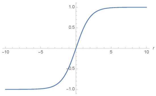
Figure 1.
The acoustic black hole (BH) profile (16) for the surface gravity .
The condition for the maximum of the term in at equal v is (see Equation (15))
where and , and this is plotted in Figure 2.
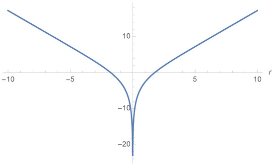
Figure 2.
Plot of the right-hand and left-hand sides of Equation (20) for .
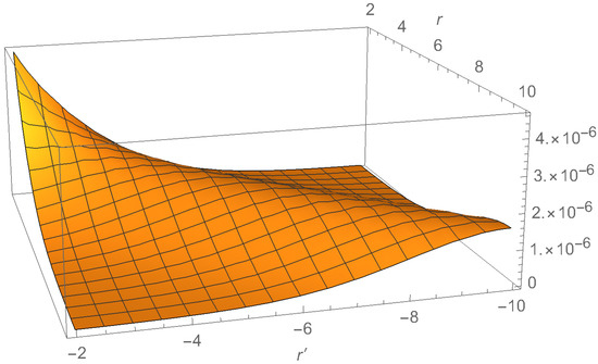
Figure 3.
The correlator, (14) for the acoustic BH model, for and .
In Figure 3, one can immediately notice the presence of the expected peak signaling the correlations between the Hawking particles and their partners. The location of the peak is indeed along Equation (20) for a sufficiently large r (and ), where the prefactors rapidly approach one. For the points near the horizon, the situation is different. To see what happens in the horizon vicinity, in Figure 4, we plot as a function of r for various fixed values of .
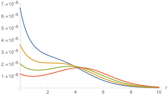
Figure 4.
The correlator for the acoustic BH model for and as a function of r, as well as for fixed (blue line), (orange), (green) and (red).
The peak appears at only for points For the points located closer to the horizon, no peak appears [10]: the maximum disappears and it merges in the light-cone singularity at the coincidence points (i.e., ). This behaviour corroborates the idea that the Hawking particle and its corresponding partner emerge on shell out of a region of a nonvanishing extension across the horizon, which is called the “quantum atmosphere” [11,12,13]. In this case, it has an extension of order . Inside this quantum atmosphere, the vacuum polarization and Hawking radiation are comparable and, so, cannot be disentangled.
4. Schwarzschild BH
The Schwarzschild BH is characterized by
where m is the mass of the BH and . The horizon is at m, and its surface gravity is , while is the physical singularity. In this case,
and
The condition, , is shown in Figure 5, and reads:
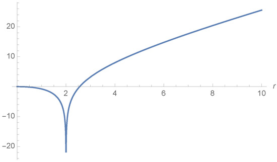
Figure 5.
Plot of both sides of Equation (24) for the BH mass .
The 3-dimensional (3D) plot of the correlator is given in Figure 6. One does not see any structure [14]. The expected peak does not show up. This can also be seen in Figure 7, where is plotted as a function of r for various values of .
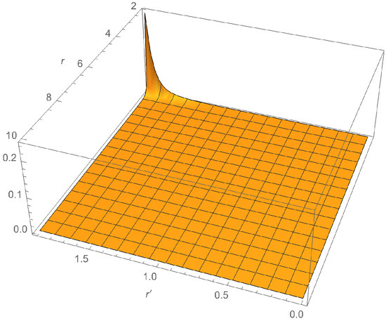
Figure 6.
The 3-dimensional (3D) plot of for the Schwarzschild BH ().
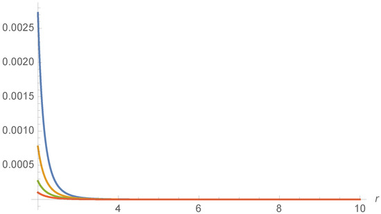
Figure 7.
for the Schwarzschild BH (), shown as a function of r for different fixed values of m (blue line), m (orange), m (green) and m (red).
The reason for the negative result obtained is not that the correlations between the Hawking particles and their partners do not exist in this case, but rather it is that the correlations do not show up in the equal time correlators. Looking at Figure 5, one can see that the solution of Equation (24) exists only for the tiny interval of values of r outside the horizon, where the vacuum contribution is not negligible. On the other hand, when the Hawking particle emerges on shell out of the vacuum fluctuation, the corresponding particle has been already swallowed by the singularity and, thus, the correlations do not show up. To reveal the correlations, one has to intercept the partner before the latter becomes swallowed by the singularity. To this end, the correlator has to be computed not at equal times, , but at . In Figure 8, we show 3D plot of for m, and show the same correlator as a function of r for several fixed values of in Figure 9. The peak indeed appears along .
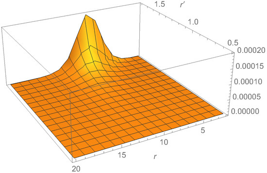
Figure 8.
The 3D plot of for the Schwarzschild BH () and m.
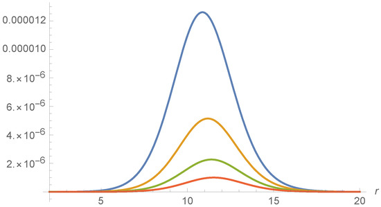
Figure 9.
for the Schwarzschild BH (), m, as a function of r for the fixed values of m (blue line), m (orange), m (green) and m (red).
5. The Callan–Giddings–Harvey–Strominger (CGHS) BH
We have seen that, in a BH, in order to see the correlations, one has to catch the partner before it reaches the singularity. Here, we consider a BH metric where the singularity is pushed at . The CGHS BH we discuss below appears as a solution of a 2D dilaton gravity theory (see [15] for details), and its metric reads:
where is a parameter that is interpreted as a cosmological constant. Here, . The horizon is located at
and the corresponding surface gravity is . The metric has a physical singularity at , which is where the curvature diverges. For this metric, one has:
where now
and the condition reads as
Here, and . In Figure 10, we plot both sides of Equation (29). Note that the value of r corresponding to is
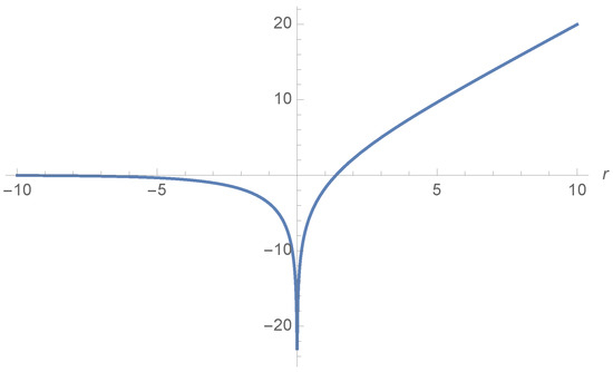
Figure 10.
Plot of both sides of Equation (29) for .
So, is correlated to a point that is still inside the quantum atmosphere.
As shown in Figure 11, when the correlator for this metric is plotted, no correlation shows up. The explanation of this negative result relies on the fact that, although the singularity is at , it is not “infinitely" far away. The proper distance,
is finite.
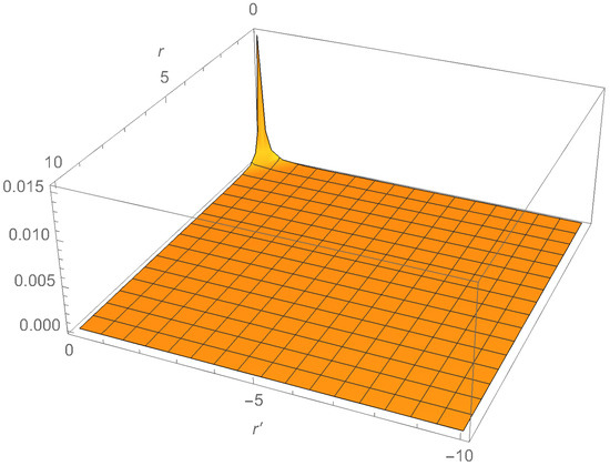
Figure 11.
for the Callan–Giddings–Harvey–Strominger (CGHS) BH, and .
The CGHS metric shown is therefore of the same behaviour found before in the Schwarzschild metric concerning the correlation across the horizon. The partner is swallowed by the singularity before the Hawking particle emerges out of the quantum atmosphere.
6. Simpson–Visser Metric
The last example concerns a BH metric where the singularity is removed, thus where one has a “regular BH”. Among many proposals in the literature for this kind of BHs, we confined our attention to quite a simple metric, the so called Simpson–Visser metric [16], for which
where a is a parameter that regularizes the singularity, and which we chose such that m. For , one has the Schwarzschild metric with a singularity at . For , the space–time surface is regular and represents a bounce that separates one asymptotically flat Universe (where ) from an identical copy with .
corresponds to a pair of horizons ( m). The part of the Penrose diagram of the Simpson–Visser metric covered by the coordinates is given in Figure 12.
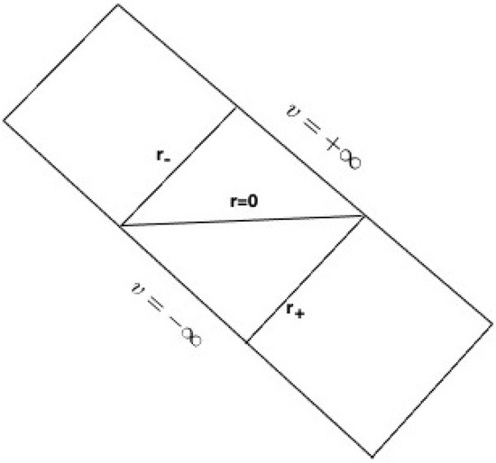
Figure 12.
Penrose diagram of the part of the Simpson–Visser metric covered by the coordinates. See text for details.
For this metric,
and
Figure 13a represents the trajectories of a Hawking particle (solid line) partner (dashed line) pair, which is created near . Meanwhile, Figure 13b represents a pair created near . All particles propagate along .
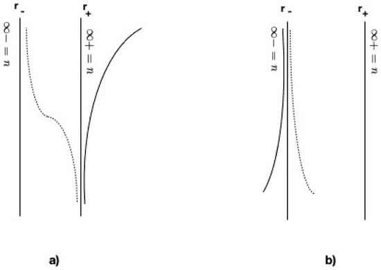
Figure 13.
The trajectories of a pair of the Hawking particle (solid line) and the partner (dashed line) created near (a) and (b) ; see Equation (33).
One can see that, in the first case (Figure 13a), while the Hawking particle goes away to infinity, the partner piles up along . In the second case, both the Hawking particle and the partner pile up along . In this situation, one recalls what happens in the interior of the Reissner–Nordström BH. As in latter case case, one has to introduce two Kruskal coordinates: one been regular on :
where the subscript ’−’ refers to , and the subscript ’+’ refers to ; and the other one been regular on :
where now the subscript ’+’ refers to , and the subscript ’−’ to . is the absolute value of the surface gravity being the same for both horizons:
Note that the coordinate is regular on , where , but is singular on , where .
One can define a Unruh state, , by expanding the quantum field in modes like Equation (10), where . Similarly, is defined by the expansion (10), where now . The singularities of the coordinates (36) and (37) induce singularities in the corresponding modes; for example, is singular on . However, as the surface gravity is the same in absolute values, one can show that the quantum stress tensor is the same in both states , and that it is regular on both horizons (see Appendix A). Also, the correlator, being an even function of the surface gravity (see Equation (14)), is the same in .
The extremal of the -term is now given by , which reads:
(plotted in Figure 14), where the condition and is for the case of Figure 13a, while the condition and is for Figure 13b ( from Figure 13a and Figure 14, one sees that the condition (39) is always satisfied, but the points with are correlated with the corresponding partners that are piling up close to ).
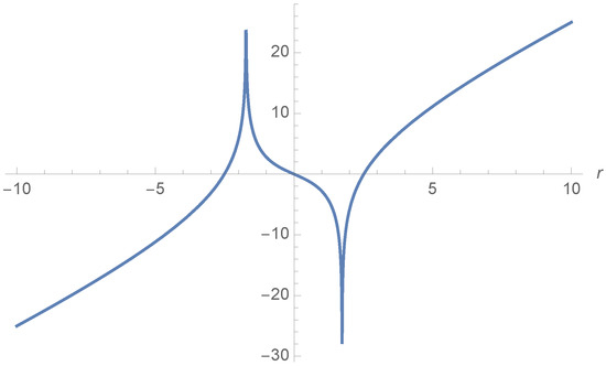
Figure 14.
Plot of both sides of Equation (39), where , , ).
The corresponding correlator (for a preliminary study see [17]) is graphically represented in Figure 15.
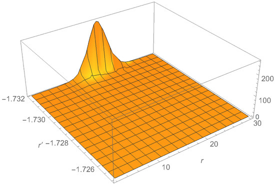
Figure 15.
for the Simpson–Visser BH, and and ).
One can further appreciate this by examining the correlator at the fixed inner point, , as shown in Figure 16. The values of r and for the peak are in good agreement with the expected one, , which is given, at equal times, by Equation (39).
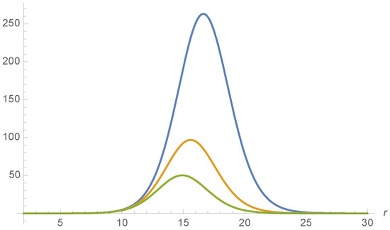
Figure 16.
for the Simpson–Visser BH, and and ), as a function of r at the fixed values of (blue curve), (orange) and (green).
On the contrary, the correlator corresponding to Figure 13b does not show any sign of correlations, see Figure 17. This is understandable since both the Hawking particle and the partner now pile up along , which remains well inside the quantum atmosphere, i.e., where the correlator is dominated by the coincidence limit singularity.
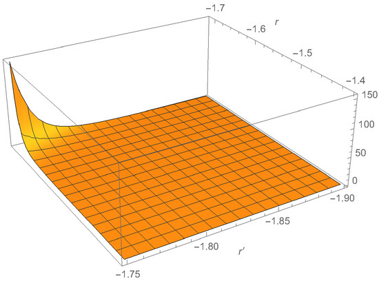
Figure 17.
for the Simpson–Visser BH, and , ), for the case of Figure 13b.
7. Conclusions
Hawking radiation is a genuine pair (particle–partner) production process that is expected to be a general feature of gravitational BHs, as well as of the analog ones realized in condensed matter systems. It is indeed in these latter cases (and only in those cases) that the existence of this radiation has been (indirectly) observed. This observation consists of detecting the correlations across the sonic horizon between the Hawking particles and their entangled partners.
In this paper, we analyzed various examples of BH space–time metrics to see if and where these correlations show up. Indeed, they can be hidden by the geometrical structure of the underlying space–time, like the presence of singularities or inner horizons that were shown explicitly here. We have seen that singularities (without inner horizons) swallow the partners before the corresponding Hawking particles emerge on shell out of the quantum atmosphere, which obscures the existing correlations. On the other hand, inner horizons produce a piling up of the partners along them by enhancing and strongly localizing the correlations.
Author Contributions
R.B. and A.F. contributed equally to this work. All authors have read and agreed to the published version of the manuscript.
Funding
A.F. acknowledges partial financial support by the Spanish Ministerio de Ciencia e Innovación Grant No. PID2020–116567 GB-C21 funded by Grant No. MCIN/AEI/10.13039/501100011033, and the Project No. PROMETEO/2020/079 (Generalitat Valenciana).
Data Availability Statement
Not applicable.
Conflicts of Interest
The authors declare no conflict of interest.
Appendix A
Consider a 2D space–time metric,
where u and v are null coordinates, which are mainly expressed in terms of a Schwarzschild-like time, t, as
and
is supposed to vanish at (outer horizon) and at (inner horizon). The expectation values of the stress-energy tensor operator, , for a quantum massless scalar field in the Unruh state are defined by expanding the quantum field on the basis of , where
and is the surface gravity of the horizon : [18]
where a prime indicates a derivative with respect to r, and is the Schwarzian derivative between and u, which reads as
is regular on the outer horizon (), if it is finite in a regular frame there. As such, we have
Equations (A10)–(A12) imply that the stress tensor is regular in a free falling frame across the horizon.
One immediately sees that if is finite on the horizon with its derivatives up to the second, conditions (A11) and (A12) are satisfied (see Equations (A6) and (A7)). Concerning the component (see Equation (A8)), note that the leading order is , i.e., the vacuum polarization and Hawking radiation cancel out on the horizon. Furthermore, by taking the derivative of Equation (A8), and evaluating the latter on the horizon, one has:
So vanishes on the horizon as , and the condition (A10) is also satisfied.
If there is another horizon (the inner one at ), the regularity there requires conditions similar to Equations (A10)–(A12) to be satisfied; one just has to consider the limit . No issue with Equations (A11) and (A12) arises, while concerning Equation (A10), one finds from Equation (A8):
which is nonvanishing whenever , such as in a non extremal Reissner–Nordström BH, for example. This makes condition (A10) been not satisfied, and hence is singular on . One can define an Unruh vacuum with respect to the Kruskal coordinate on , i.e.,
and, similarly, one finds regularity on , but on :
thus making singular on .
In the case of the Simpson–Visser metric, one has two horizons indeed, the outer one at , but then for this space–time. So, now both and are indeed regular on both () and (). However, a singularity appears on the Cauchy horizon and . For a regularity, it would require
Equation (A19) is not satisfied since
If, on the other hand, one constructs the Hartle–Hawking states,
where
one finds that these states are regular all over the space–time, and, thus, they describe a BH that is in a thermal equilibrium with the thermal radiation at the Hawking temperature,
References
- Hawking, S.W. Black hole explosions? Nature 1974, 248, 30–31. [Google Scholar] [CrossRef]
- Hawking, S.W. Particle creation by black holes. Commun. Math. Phys. 1975, 43, 199–200. [Google Scholar] [CrossRef]
- Steinhauer, J. Observation of quantum Hawking radiation and its entanglement in an analogue black hole. Nat. Phys. 2016, 12, 959–965. [Google Scholar] [CrossRef]
- De Nova, J.R.M.; Golubkov, K.; Kolobov, V.I.; Steinhauer, J. Observation of thermal Hawking radiation and its temperature in an analogue black hole. Nature 2019, 569, 688–691. [Google Scholar] [CrossRef] [PubMed]
- Kolobov, V.I.; Golubkov, K.; de Nova, J.R.M.; Steinhauer, J. Spontaneous Hawking radiation and beyond: Observing the time evolution of an analogue black hole. Nat. Phys. 2021, 17, 362–367. [Google Scholar] [CrossRef]
- Balbinot, R.; Fabbri, A.; Fagnocchi, S.; Recati, A.; Carusotto, I. Nonlocal density correlations as a signature of Hawking radiation from acoustic black holes. Phys. Rev. A 2008, 78, 021603. [Google Scholar] [CrossRef]
- Carusotto, I.; Fagnocchi, S.; Recati, A.; Balbinot, R.; Fabbri, A. Numerical observation of Hawking radiation from acoustic black holes in atomic Bose–Einstein condensates. New J. Phys. 2008, 10, 103001. [Google Scholar] [CrossRef]
- Parentani, R. From vacuum fluctuations across an event horizon to long distance correlations. Phys. Rev. D 2010, 82, 025008. [Google Scholar] [CrossRef]
- Unruh, W.G. Notes on black-hole evaporation. Phys. Rev. D 1976, 14, 870–892. [Google Scholar] [CrossRef]
- Schutzhold, R.; Unruh, W.G. Quantum correlations across the black hole horizon. Phys. Rev. D 2010, 81, 124033. [Google Scholar] [CrossRef]
- Giddings, S.B. Hawking radiation, the Stefan–Boltzmann law, and unitarization. Phys. Lett. B 2016, 754, 39–42. [Google Scholar] [CrossRef]
- Dey, R.; Liberati, S.; Mirzaiyan, Z.; Pranzetti, D. Black hole quantum atmosphere for freely falling observers. Phys. Lett. B 2019, 797, 134828. [Google Scholar] [CrossRef]
- Ong, Y.C.; Good, M.R.R. Quantum atmosphere of Reissner-Nordström black holes. Phys. Rev. 2020, 2, 033322. [Google Scholar] [CrossRef]
- Balbinot, R.; Fabbri, A. Quantum correlations across the horizon in acoustic and gravitational black holes. Phys. Rev. D 2022, 105, 045010. [Google Scholar] [CrossRef]
- Callan, C.G., Jr.; Giddings, S.B.; Harvey, J.A.; Strominger, A. Evanescent black holes. Phys. Rev. D 1992, 45, R1005–R1009. [Google Scholar] [CrossRef] [PubMed]
- Simpson, A.; Visser, M. Black-bounce to traversable wormhole. J. Cosmol. Astropart. Phys. 2019, 2019, 42. [Google Scholar] [CrossRef]
- Fontana, M.; Rinaldi, M. Stress-energy tensor correlations across regular black holes horizons. arXiv 2013, arXiv:2302.08804. [Google Scholar] [CrossRef]
- Birrell, N.D.; Davies, P.C.W. Quantum Fields in Curved Space; Cambridge University Press: New York, NY, USA, 1984. [Google Scholar] [CrossRef]
Disclaimer/Publisher’s Note: The statements, opinions and data contained in all publications are solely those of the individual author(s) and contributor(s) and not of MDPI and/or the editor(s). MDPI and/or the editor(s) disclaim responsibility for any injury to people or property resulting from any ideas, methods, instructions or products referred to in the content. |
© 2023 by the authors. Licensee MDPI, Basel, Switzerland. This article is an open access article distributed under the terms and conditions of the Creative Commons Attribution (CC BY) license (https://creativecommons.org/licenses/by/4.0/).