Combining the Pre-Trained Model Roberta with a Two-Layer Bidirectional Long- and Short-Term Memory Network and a Multi-Head Attention Mechanism for a Rice Phenomics Entity Classification Study

Abstract

At a time when global food security is challenged, the importance of phenomics research on rice, as a major food crop, has become more and more prominent. In-depth analysis of rice phenotypic characteristics is of key importance to promote the genetic improvement of rice and sustainable agricultural development. However, it is a challenging task to accurately identify and classify entities from the huge amount of rice phenotypic data. In this study, a deep learning model based on Roberta-two-layer BiLSTM-MHA was innovatively constructed for rice phenomics entity classification. Firstly, with the powerful language comprehension capability of the pre-trained Roberta model, deep feature extraction was performed on the rice phenotype text data to capture the underlying semantic information in the text. Next, the contextual information is comprehensively modelled using a two-layer bidirectional long- and short-term memory network (BiLSTM) to fully explore the long-term dependencies in the text sequences. Finally, a multi-head attention mechanism is introduced to enable the model to adaptively focus on key features at different levels, which significantly improves the classification accuracy of complex phenotypic information. The experimental results show that the model performs excellently in several evaluation metrics, with accuracy, recall, and F1-scores of 89.56%, 86.40%, and 87.90%, respectively. This research result not only provides an efficient and precise entity classification tool for rice phenomics research but also provides a comparable method for other crop phenomics analyses, which is expected to promote the technological innovation in the field of crop genetic breeding and agricultural production.

1. Introduction

In the contemporary agricultural sector, a comprehensive understanding of the intricate traits and phenotypes of crops is paramount for enhancing crop yields, fortifying resistance, and cultivating novel varieties. Rice, a staple food of global significance, has been the focus of substantial research in the domain of phenomics [1]. The objective of rice phenomics is to systematically examine the observable characteristics of rice throughout its growth cycle, encompassing morphological, physiological, and biochemical traits [2]. These traits are intricately linked to factors such as rice yield, quality, and adaptation to diverse environments.

The classification of entities in the field of rice phenomics constitutes a fundamental task, involving the accurate identification and classification of various entities related to rice phenotypes. For instance, entities such as ‘plant height’, ‘spike length’, ‘number of grains per spike’, and ‘chlorophyll content’ are important phenotypic characters. The accurate classification of these entities can provide valuable information for rice breeding, cultivation management, and ecological studies. The correct classification of these entities enables researchers to analyse the relationship between different phenotypes and genetic and environmental factors more comprehensively [3], which is essential for the promotion of the breeding of high-yielding, high-quality, and stress-resistant rice varieties.

The conventional approaches employed for the classification of rice phenomics entities predominantly entail the utilisation of manual annotation and rudimentary machine learning algorithms. Manual annotation is an arduous and protracted process that is susceptible to human error. Moreover, the implementation of simple machine learning algorithms, such as support vector machines (SVMs) [4] and decision trees [5], necessitates a substantial volume of meticulously pre-processed data and sophisticated feature engineering. These methodologies encounter challenges in effectively handling the intricate and multifaceted nature of rice phenomics data. These methods frequently encounter difficulties in capturing intricate semantic relationships and contextual information present within the data. This often results in a comparatively low level of accuracy and suboptimal generalisation [6].

The advent of deep learning technology has precipitated the application of a plethora of neural network models to the domain of entity classification [7]. Dai H et al. [8] proposed using a masked language model to obtain training data for hyperfine entity classification. The model inputs contextual entities into the masked language model to predict contextually relevant hypernyms for the entities, which can serve as entity category labels. These automatically generated labels can significantly enhance the performance of ultra-fine-grained entity classification models. Ding N et al. [9] investigated the application of cue learning in supervised, sample-less, and zero-shot learning for fine-grained entity classification. The proposed model suggests a straightforward yet efficient method for learning cues by creating linguistic expressions and templates for entities and conducting masked language modelling. To solve the problem of label noise in remotely supervised fine-grained entity classification, Xu et al. [10] proposed a semi-supervised learning method with a mixture of label smoothing and pseudo-labelling for remotely supervised fine-grained entity classification to improve classification accuracy. In an attempt to address the fact that the spanning of the methods ignores the local features inside the entity as well as the relative positional features between the head and tail markers, Deng et al. [11] used a convolutional block attention module and rotational position embedding to enhance the local and relative position features for the classification of the entities. Zhang et al. [12] introduced document-level entity-based extension features to construct a financial entity classification model to address the characteristics of lengthy entities, challenging delineate boundaries and varied expressions. Yuan et al. [13] proposed the ERNIE-ADV-BiLSTM-AT-CRF model to mitigate the impact of noise on model training by employing adversarial training as a regularisation method. The BiLSTM-CRF model incorporates self-attention mechanisms to capture crucial features for entity classification, thereby enhancing the accuracy of extracting food safety-related entity classifications from unnormalized text. To overcome the limitations of the multi-label space and the lack of integration of domain knowledge in traditional Chinese medicine (TCM) symptom ontology, Hu et al. [14] integrated the traditional entity recognition technique of bidirectional encoder representation (BERT) + bidirectional long- and short-term memory (Bi-LSTM) + a conditional random field (CRF) with a multi-label classification strategy. This approach effectively addresses the complex label dependency problem in textual data, enabling the extraction of key entity features even when identifying relationships between different label categories. It is shown that the model exhibits excellent performance in multi-label symptom extraction and also significantly improves the operational efficiency and accuracy of the model. Nonetheless, challenges persist in the domain of classifying entities for rice phenomics. To illustrate this point, it should be noted that the majority of extant deep learning models have been designed for general-purpose natural language processing or image recognition tasks. Consequently, when these models are applied directly to rice phenomics, there is a risk that they may not be able to fully utilise the unique features and semantic information of rice-related data.

In the domain of agricultural information extraction, the automatic identification of entities and their relationships from the text related to rice features has emerged as a pivotal research direction. The accurate classification of rice features is imperative for achieving efficient data integration and unified management. To this end, this study proposes a novel model based on Roberta’s two-layer BiLSTM attention mechanism, with the objective of attaining high-precision classification of rice features.

Although BiLSTM linguistic models have been applied before, for example, N. A. P. Masaling, and D. Suhartono et al. [15] have trained three BiLSTM models using three datasets from SemEval-2022 Task 10 “Structured Sentiment Analysis” (SSA) [16]. However, the Roberta-based two-layer BiLSTM-MHA model proposed in this study makes a new attempt in architectural combination and functional implementation for rice phenomics entity classification. While traditional BiLSTM models mainly rely on a two-way loop structure to capture sequence information, this model introduces the multi-head attention (MHA) mechanism. This mechanism enables the model to capture the semantic associations between different locations in the text more flexibly and efficiently, which significantly enhances the ability to handle complex semantic relationships. Meanwhile, the combination of the model with Roberta’s pre-trained model, which has strong semantic characterisation capabilities, demonstrates the advantages of the model over the previous single BiLSTM model, especially in terms of accuracy and efficiency, when dealing with specific natural language processing tasks related to rice features. Finally, the focal loss function is chosen to optimise model training and mitigate the negative impact of category label imbalance. For this reason, this novel model is proposed in this study, aiming to achieve high-precision classification of rice features. The specific research is as follows.

(1)

The feature extraction phase: the introduction of the Roberta pre-trained model

The pre-trained Roberta model is used for in-depth feature extraction of text data related to rice phenomics. The model is pre-trained on a large-scale unsupervised corpus, which is capable of capturing rich semantic information and transforming the text data into high-quality feature vectors, thus laying a solid foundation for subsequent processing.

(2)

The sequence information capturing stage: using a two-layer BiLSTM network

The feature vectors extracted by Roberta are fed into a two-layer BiLSTM network. The two-layer BiLSTM can process the sequence data in both forward and reverse directions and effectively capture the long-distance dependencies in the text sequence. The first-layer BiLSTM initially learns the features and patterns of the sequence, and the second-layer BiLSTM further mines more complex information on the basis of this so as to understand the semantic and contextual information of the text more comprehensively.

(3)

The key information focusing stage: applying the multi-head attention mechanism

The multi-head attention mechanism is introduced on the basis of the output results of the two-layer BiLSTM. The multi-head attention mechanism allows the model to focus on different parts of the input sequence in parallel in several different representation subspaces, adaptively assigning different attention weights to information at different locations. In this way, the model is able to focus on the information that is most critical to the entity classification task, improving the ability to perceive and utilise the important features in the text, as well as improving the accuracy and robustness of the classification.

(4)

The model integration and classification phase

Roberta, the two-layer BiLSTM and the multi-head attention mechanism are organically integrated to form a complete model architecture. The model can make full use of the advantages of each component to analyse and understand rice phenomics entities from different perspectives. Ultimately, the output based on the model achieves accurate classification of rice phenomics entities, which provides strong support for subsequent agricultural research and data management.

The paper is structured as follows: Section 2 outlines the research methodology and data sources, as well as the experimental setup and data collection techniques. Section 3 provides a comprehensive analysis and discussion of the experimental results, as well as the statistics and interpretation of the experimental data. The Section 4 summarises the current work and outlines future research directions.

2. Materials and Methods

2.1. Data Source

Aiming to address the scarcity of publicly available datasets in the field of rice phenomics. There are two sources of data for this study. First, this study will create the rice phenomics entity classification corpus by extracting information from web resources and manually curating excerpts using the Scrapy crawler framework. Additionally, the study will compile the rice phenomics entity classification dataset by incorporating insights from plant protection experts. This paper utilises the Scrapy crawler framework as a tool for data collection. The framework fully utilises processor resources and efficiently retrieves structured data. Its capacity for distributed crawling makes it particularly adept at managing extensive rice phenomics data collections. Secondly, for literature supplementation, in order to ensure the accuracy and authority of the data, content from specialised studies in the field of rice phenomics was selected for supplementation. The literature contains a large number of specialised terms and profound knowledge in rice phenomics, providing a strong guarantee for the quality and professionalism of the dataset.

2.2. Data Preprocessing

2.2.1. Entity Identification

A rice phenomics corpus, acquired through a crawling framework, undergoes initial sentence and word segmentation. Following this, unnecessary stop words are removed from the text. In the end, it was organised to contain a total of 4000 rice phenomics texts. A team consisting of domain experts and professional annotators was formed in the course of the study, and before the formal annotation step, the team members worked together to formulate a detailed annotation guideline, which clearly explained the definitions of various types of entities, the annotation rules, and the precautions to be taken in order to ensure the accuracy and consistency of the annotation. For example, different types of entities were defined in terms of multiple dimensions such as semantics, syntax, and context. Then, the process utilises specialised agricultural dictionaries obtained from the Agricultural Dictionary (https://dict.bioon.com/) (accessed on 15 July 2024) in conjunction with the Chinese Natural Language Processing tool, Hanlp, to identify entities within rice phenomics-related phrases, thereby facilitating the extraction of relevant entities. Figure 1 illustrates an entity recognition example for text data related to rice.

Figure 1. An example of named-entity recognition.

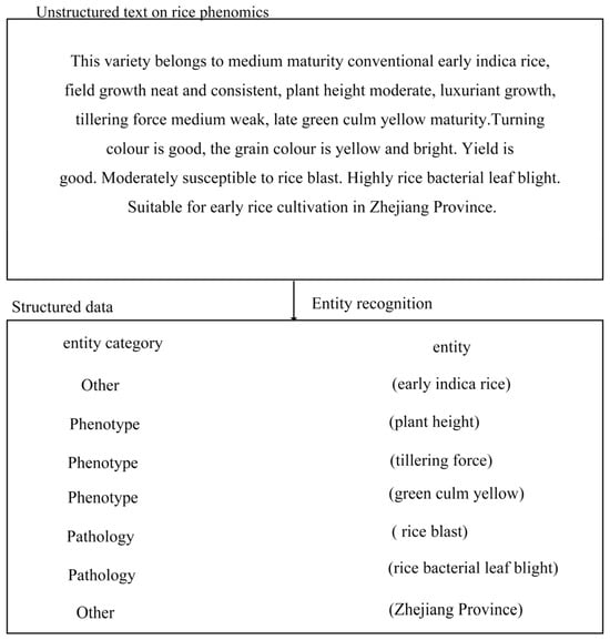
Figure 1. An example of named-entity recognition.

After defining the types of rice phenomics entities, rice phenomics contains a lot of specialised knowledge, so manual annotation was used. In this study, Label-Studio (https://labelstud.io/) (accessed on 23 September 2024) was chosen as the labelling tool, which provides an intuitive interface that facilitates rapid labelling and reviews. The annotation is shown in Figure 2; after the annotation, it is exported and saved in JSON format; using the relevant code for BIO annotation, the text data is labelled using the BIO annotation method, where B represents the starting position of the entity, I represents the continuation of the entity to the end of the entity, and O indicates that it does not belong to any entity. Finally, it is saved in CSV file format. The label information mainly consists of entity types and entity boundaries, as shown in Table 1.

Figure 2. Label-Studio labelling process.

Figure 2. Label-Studio labelling process.

In order to ensure the consistency of the annotation, several rounds of annotations were carried out, and after the completion of the first annotation, several rounds of reviews were carried out manually. An example of BIO labelling is shown in Figure 3.

Table 1. Label symbol representation of entities in rice phenomics.

Entity Type	Entity Beginning	Entity Middle	Entity Ending
Chemical	B-Chemical	I-Chemical	I-Chemical
Gene	B-Gene	I-Gene	I-Gene
Other	B-Other	I-Other	I-Other
Pathology	B-Pathology	I-Pathology	I-Pathology
Environment	B-Environment	I-Environment	I-Environment
Phenotype	B-Phenotype	I-Phenotype	I-Phenotype

Table 1. Label symbol representation of entities in rice phenomics.

Entity Type	Entity Beginning	Entity Middle	Entity Ending
Chemical	B-Chemical	I-Chemical	I-Chemical
Gene	B-Gene	I-Gene	I-Gene
Other	B-Other	I-Other	I-Other
Pathology	B-Pathology	I-Pathology	I-Pathology
Environment	B-Environment	I-Environment	I-Environment
Phenotype	B-Phenotype	I-Phenotype	I-Phenotype

2.2.2. Experimental Data

Text data containing entities and corresponding categories in the field of rice phenomics were collected using the Scrapy crawling technique, dividing the text into left and right contexts and entity parts. The example data of 10 entries are shown in Table 2.

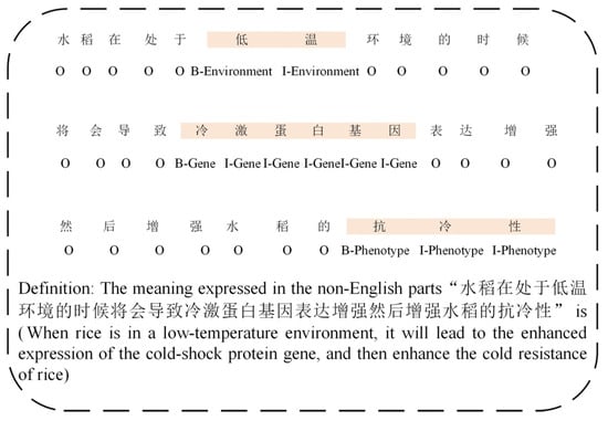
Figure 3. Example of a BIO labelling section.

Figure 3. Example of a BIO labelling section.

Table 2. Example data.

Serial Number	Text	Entity	Entity Category
1	In a high-temperature environment, rice growth is affected to a certain extent.	High-temperature environment	Environment
2	The OsMYB4 gene regulates the stress resistance of rice.	OsMYB4 gene	Gene
3	Applying nitrogen fertiliser can increase the yield of rice.	Nitrogen fertiliser	Chemical
4	After rice is infected with rice blast, the yield will drop significantly.	Rice blast	Pathology
5	The plant height of this rice plant reaches 1.2 m.	Plant height	Phenotype
6	Under the condition of sufficient irrigation, rice grows well.	Sufficient irrigation	Environment
7	The OsWRKY71 gene is related to the disease resistance of rice.	OsWRKY71 gene	Gene
8	Using carbendazim can prevent and control the diseases of rice.	Carbendazim	Chemical
9	Bacterial blight of rice is a common disease.	Bacterial blight	Pathology
10	The tiller number of this rice variety is relatively high.	Tiller number	Phenotype

Table 2. Example data.

Serial Number	Text	Entity	Entity Category
1	In a high-temperature environment, rice growth is affected to a certain extent.	High-temperature environment	Environment
2	The OsMYB4 gene regulates the stress resistance of rice.	OsMYB4 gene	Gene
3	Applying nitrogen fertiliser can increase the yield of rice.	Nitrogen fertiliser	Chemical
4	After rice is infected with rice blast, the yield will drop significantly.	Rice blast	Pathology
5	The plant height of this rice plant reaches 1.2 m.	Plant height	Phenotype
6	Under the condition of sufficient irrigation, rice grows well.	Sufficient irrigation	Environment
7	The OsWRKY71 gene is related to the disease resistance of rice.	OsWRKY71 gene	Gene
8	Using carbendazim can prevent and control the diseases of rice.	Carbendazim	Chemical
9	Bacterial blight of rice is a common disease.	Bacterial blight	Pathology
10	The tiller number of this rice variety is relatively high.	Tiller number	Phenotype

The data were pre-processed and tagged according to the entity tags. The entities in this paper are divided into six categories: chemical, genetic, others, pathological, environmental, and phenotypic. The detailed entity categories are shown in Table 3.

Table 3. Entity categories.

Entity Type	Number of Entities	Label
Chemical	433	0
Gene	1862	1
Others	1365	2
Pathology	283	3
Environment	193	4
Phenotype	1373	5

Table 3. Entity categories.

Entity Type	Number of Entities	Label
Chemical	433	0
Gene	1862	1
Others	1365	2
Pathology	283	3
Environment	193	4
Phenotype	1373	5

2.3. Model Architecture

In this paper, a classification study of rice phenome entities was conducted using Roberta–two-layer BiLSTM-MHA. The model diagram is shown in Figure 4.

The overall processing steps of the model are as follows: first, Roberta is applied to encode the left and right contexts and entities to obtain the vector representation of each character or word, and the vectors of the left and right contexts are subjected to the averaging or attention weighting operation to obtain the context features.

Then, the two-layer BiLSTM module is used to obtain the semantic coding information. Finally, the multi-head attention mechanism is used to classify the rice phenome entities.

Figure 4. Model architecture diagram.

Figure 4. Model architecture diagram.

2.3.1. Word Embedding Layer

In order to better present the input features of the acquired Chinese text, this paper adopts Roberta-wwm-ext as the pre-training model [17]. The structure of the model is shown in Figure 5. Compared to the original BERT [18] model, this model is optimised in two main aspects: The first is that it leverages the strengths of the Roberta [19] model. The second is based on the Chinese Whole Word Mask (WWM) technique.

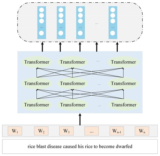
Figure 5. Structure of the Roberta model.

Figure 5. Structure of the Roberta model.

The Roberta-wwm-ext model is constructed using 12 layers of Transformers, each with 12 heads of self-attention and 768 hidden layer units [20]. The Transformer mainly consists of an encoder and a decoder, among which the self-attention mechanism is the key part, and its formula refers to Equation (1):

$$Attention(\mathrm{Q},\mathrm{K},\mathrm{V})=softmax({\displaystyle \frac{Q{\mathrm{K}}^T}{\sqrt{d_k}}})\mathrm{V}$$

(1)

In this formula, embedding is multiplied with three different weight matrices to obtain the corresponding three input matrices, i.e., Q, K, and V. Here, $d_k$ means the dimension of inputs Q and K. Based on this formula, the different weights can be derived by figuring out the ratio of the relationship between the current word vector and the other word vectors. Subsequently, these weights are weighted and summed with their corresponding sequence representations, and character representation information is finally obtained [21].

Let the input text rice phenomics be divided into the left context $C_{left}=\{w_{l1},w_{l2},\cdots ,w_{l{n}_l}\}$, entity $E=\{w_{e1},w_{e2},\cdots ,w_{em}\}$ and right context $C_{right}=\{w_{r1},w_{r2},\cdots ,w_{r{n}_r}\}$, where $n_l$, $m$, and $n_r$ are the lengths of the left context, entity, and right context, respectively. The flowchart is shown in Figure 6.

They are coded using the Roberta model to obtain the corresponding vector sequences: The left context vector sequence $V_{left}=\{v_{l1},v_{l2},\cdots ,v_{l{n}_l}\}$, where $v_{li}=R(w_{li}),i=1,2,\cdots ,n_l$. The entity vector sequence $V_e=\{v_{e1},v_{e2},\cdots ,v_{em}\}$, where $v_{ej}=R(w_{ej}),j=1,2,\cdots ,m$. The right context vector sequence $V_{right}=\{v_{r1},v_{r2},\cdots ,v_{r{n}_r}\}$, where $v_{rk}=R(w_{rk}),k=1,2,\cdots ,n_r$.

In order to compute the correlation between the left context vector and the entity vectors, this study defines a query vector $q$ (the average vector $q={\displaystyle \frac{1}{m}}{\displaystyle \sum _{j=1}^m{v}_{ej}}$ of the entity vectors). For each vector $v_{li}$ of the left context, its similarity score $s_{li}$ with the query vector $q$ can be calculated using the dot product as follows:

$$s_{li}=v_{li}^{T}q$$

(2)

In a similar manner, for each vector $v_{rk}$ in the appropriate context, its similarity score $s_{rk}$ with the query vector $q$ is

$$s_{rk}=v_{rk}^{T}q$$

(3)

The similarity scores were then converted to attention weights using the Softmax function.

The attention weight ${\alpha }_{li}$ of the left context vector $v_{li}$ is as follows:

$${\alpha }_{li}={\displaystyle \frac{\exp (s_{li})}{{\displaystyle \sum _{i^{\prime }=1}^{n_l}\exp }(s_{l{i}^{\prime }})}}$$

(4)

The attention weight ${\alpha }_{rk}$ of the right context vector $v_{rk}$ is as follows:

$${\alpha }_{rk}={\displaystyle \frac{\exp (s_{rk})}{{\displaystyle \sum _{k^{\prime }=1}^{n_r}\exp }(s_{r{k}^{\prime }})}}$$

(5)

Attention feature vector $h_{left}$ for the left context and attention feature vector $h_{right}$ for the right context are obtained using weighted summation:

$$h_{left}={\displaystyle \sum _{i=1}^{n_l}{\alpha }_{li}}{v}_{li}$$

(6)

$$h_{right}={\displaystyle \sum _{k=1}^{n_r}{\alpha }_{rk}}{v}_{rk}$$

(7)

The attention feature vector $h_{left}$ of the left context, the mean vector $h_e={\displaystyle \frac{1}{m}}{\displaystyle \sum _{j=1}^m{v}_{ej}}$ of the sequence of entity vectors, and the attention feature vector $h_{right}$ of the right context are spliced to obtain the sequence of feature vectors $H^R$:

$$H^R=[h_{left};h_e;h_{right}]$$

(8)

Figure 6. Flowchart of word vectors performed using Roberta.

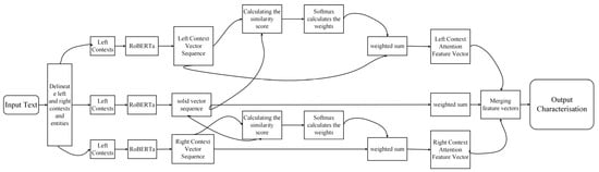
Figure 6. Flowchart of word vectors performed using Roberta.

2.3.2. Sequence Information Capture Stage

The feature vector sequence $H^R$ extracted using Roberta is inputted into a two-layer BiLSTM network, which consists of a forward LSTM and a backward LSTM, and is able to process the sequence data in both forward and backward directions, effectively capturing the long-distance dependencies in the text sequence [22]. The structure of the LSTM is shown in Figure 7.

The first-layer BiLSTM receives the sequence of feature vectors $H^R$ output by Roberta and performs preliminary feature learning on them. Let the hidden state of the forward LSTM be ${\overrightarrow{h}}_t^1$ and the hidden state of the backward LSTM be ${\overleftarrow{h}}_t^1$. The forward hidden state ${\overrightarrow{h}}_t^1$ and the backward hidden state ${\overleftarrow{h}}_t^1$ at time $t$ can be computed using the following equation:

The forward LSTM is as follows:

$${\overrightarrow{i}}_t^1=\sigma (W_{ii}^1{h}_{t-1}^R+W_{hi}^1{\overrightarrow{h}}_{t-1}^1+b_i^1)$$

(9)

$${\overrightarrow{f}}_t^1=\sigma (W_{if}^1{h}_{t-1}^R+W_{hf}^1{\overrightarrow{h}}_{t-1}^1+b_f^1)$$

(10)

$${\overrightarrow{o}}_t^1=\sigma (W_{io}^1{h}_{t-1}^R+W_{ho}^1{\overrightarrow{h}}_{t-1}^1+b_o^1)$$

(11)

$${\overrightarrow{c}}_t^1={\overrightarrow{f}}_t^1\odot {\overrightarrow{c}}_{t-1}^1+{\overrightarrow{i}}_t^1\odot {\overrightarrow{g}}_t^1$$

(12)

$${\overrightarrow{h}}_t^1={\overrightarrow{o}}_t^1\odot \tanh ({\overrightarrow{c}}_t^1)$$

(13)

The backward LSTM is as follows:

$${\overleftarrow{i}}_t^1=\sigma (W_{ii}^1{h}_{t+1}^R+W_{hi}^1{\overleftarrow{h}}_{t+1}^1+b_i^1)$$

(14)

$${\overleftarrow{f}}_t^1=\sigma (W_{if}^1{h}_{t+1}^R+W_{hf}^1{\overleftarrow{h}}_{t+1}^1+b_f^1)$$

(15)

$${\overleftarrow{o}}_t^1=\sigma (W_{io}^1{h}_{t+1}^R+W_{ho}^1{\overleftarrow{h}}_{t+1}^1+b_o^1)$$

(16)

$${\overleftarrow{g}}_t^1=\tanh (W_{ig}^1{h}_{t+1}^R+W_{hg}^1{\overleftarrow{h}}_{t+1}^1+b_g^1)$$

(17)

$${\overleftarrow{c}}_t^1={\overleftarrow{f}}_t^1\odot {\overleftarrow{c}}_{t+1}^1+{\overleftarrow{i}}_t^1\odot {\overleftarrow{g}}_t^1$$

(18)

$${\overleftarrow{h}}_t^1={\overleftarrow{o}}_t^1\odot \tanh ({\overleftarrow{c}}_t^1)$$

(19)

Figure 7. Structure of the LSTM model.

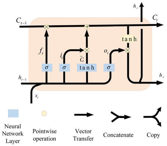
Figure 7. Structure of the LSTM model.

• where $\sigma$ is the sigmoid function, $\tanh$ is the hyperbolic tangent function, $\odot$ denotes element-by-element multiplication, $W$ is the weight matrix, and $b$ is the bias vector. The forward and backward hidden states are spliced together to obtain the output $h_t^1=[{\overrightarrow{h}}_t^1;{\overleftarrow{h}}_t^1]$ of the first-layer BiLSTM, and the output sequence of the whole first-layer BiLSTM is $H^1=[h_1^1,h_2^1,\cdots ,h_n^1]$.

The first-layer BiLSTM initially learns the features and patterns of the sequence, and the second-layer BiLSTM further mines more complex information on this basis. The computation process of the second-layer BiLSTM is similar to that of the first layer, but the input is the output of the first layer $H^1$. Let the hidden state of the second-layer forward LSTM be ${\overrightarrow{h}}_t^2$, and let the hidden state of the backward LSTM be ${\overleftarrow{h}}_t^2$; then, the forward hidden state ${\overrightarrow{h}}_t^2$ and the backward hidden state ${\overleftarrow{h}}_t^2$ in the $t$th moment can be computed using the following formula:

The forward LSTM is as follows:

$${\overrightarrow{i}}_t^2=\sigma (W_{ii}^2{h}_{t-1}^1+W_{hi}^2{\overrightarrow{h}}_{t-1}^2+b_i^2)$$

(20)

$${\overrightarrow{f}}_t^2=\sigma (W_{if}^2{h}_{t-1}^1+W_{hf}^2{\overrightarrow{h}}_{t-1}^2+b_f^2)$$

(21)

$${\overrightarrow{o}}_t^2=\sigma (W_{io}^2{h}_{t-1}^1+W_{ho}^2{\overrightarrow{h}}_{t-1}^2+b_o^2)$$

(22)

$${\overrightarrow{g}}_t^2=\tanh (W_{ig}^2{h}_{t-1}^1+W_{hg}^2{\overrightarrow{h}}_{t-1}^2+b_g^2)$$

(23)

$${\overrightarrow{c}}_t^2={\overrightarrow{f}}_t^2\odot {\overrightarrow{c}}_{t-1}^2+{\overrightarrow{i}}_t^2\odot {\overrightarrow{g}}_t^2$$

(24)

$${\overrightarrow{h}}_t^2={\overrightarrow{o}}_t^2\odot \tanh ({\overrightarrow{c}}_t^2)$$

(25)

The backward LSTM is as follows:

$${\overleftarrow{i}}_t^2=\sigma (W_{ii}^2{h}_{t+1}^1+W_{hi}^2{\overleftarrow{h}}_{t+1}^2+b_i^2)$$

(26)

$${\overleftarrow{f}}_t^2=\sigma (W_{if}^2{h}_{t+1}^1+W_{hf}^2{\overleftarrow{h}}_{t+1}^2+b_f^2)$$

(27)

$${\overleftarrow{o}}_t^2=\sigma (W_{io}^2{h}_{t+1}^1+W_{ho}^2{\overleftarrow{h}}_{t+1}^2+b_o^2)$$

(28)

$${\overleftarrow{g}}_t^2=\tanh (W_{ig}^2{h}_{t+1}^1+W_{hg}^2{\overleftarrow{h}}_{t+1}^2+b_g^2)$$

(29)

$${\overleftarrow{c}}_t^2={\overleftarrow{f}}_t^2\odot {\overleftarrow{c}}_{t+1}^2+{\overleftarrow{i}}_t^2\odot {\overleftarrow{g}}_t^2$$

(30)

$${\overleftarrow{h}}_t^2={\overleftarrow{o}}_t^2\odot \tanh ({\overleftarrow{c}}_t^2)$$

(31)

The forward and backward hidden states are spliced together to obtain the output $h_t^2=[{\overrightarrow{h}}_t^2;{\overleftarrow{h}}_t^2]$ of the second-layer BiLSTM, and the output sequence of the whole second-layer BiLSTM is $H^2=[h_1^2,h_2^2,\cdots ,h_n^2]$.

Through the processing of the two-layer BiLSTM, its structure is shown in Figure 8. The model is able to understand the semantic and contextual information of the rice phenomics text more comprehensively, providing richer and more accurate feature representations for the subsequent entity classification task.

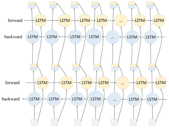
Figure 8. Structure of two-layer BiLSTM.

Figure 8. Structure of two-layer BiLSTM.

2.3.3. Key Message Focus Stage

A multi-head attention mechanism is introduced to the results of the two-layer BiLSTM output [23]. The multi-head attention mechanism allows the model to focus on different parts of the input sequence in parallel in several different representation subspaces, adaptively assigning different attention weights to information at different locations. In this way, the model is able to focus on the information that is most critical to the entity classification task, enhance the ability to perceive and utilise important features in the text, and improve the accuracy and robustness of the classification.

Principle of computing single-head attention: Given the output sequence $H^2=[h_1^2,h_2^2,\cdots ,h_n^2]$ of the second BiLSTM layer, where $h_t^2\in {ℝ}^{2d_{lstm}}$ ($d_{lstm}$ is the hidden layer dimension of each LSTM direction; $ℝ$ stands for the set of real numbers and contains all rational numbers (e.g., integers and fractions) and irrational numbers), in order to compute the attention, we first pass $H^2$ through three different linear transformations to obtain the query matrix $Q$, the key matrix $K$, and the value matrix $V$, respectively:

$$Q=H^2{W}^Q$$

(32)

$$K=H^2{W}^K$$

(33)

$$V=H^2{W}^V$$

(34)

where $W^Q\in {ℝ}^{2d_{lstm}\times d_{att}}$, $W^K\in {ℝ}^{2d_{lstm}\times d_{att}}$, and $W^V\in {ℝ}^{2d_{lstm}\times d_{att}}$ are the learnable weight matrices and $d_{att}$ is the dimension of the attention representation.

Then, the attention score is computed. For queries $q_i$ (row $i$ of $Q$) and key $k_j$ (row $j$ of $K$), the attention score $e_{ij}$ can be computed using the dot product:

$$e_{ij}={\displaystyle \frac{q_i{k}_j^T}{\sqrt{d_{att}}}}$$

(35)

The division by $\sqrt{d_{att}}$ here is to prevent the dot product result from being too large and to avoid the problem of vanishing or exploding gradients.

Next, the Softmax function is used to transform the attention score into the attention weight ${\alpha }_{ij}$:

$${\alpha }_{ij}={\displaystyle \frac{\exp (e_{ij})}{{\displaystyle \sum _{k=1}^n\exp }(e_{ik})}}$$

(36)

Finally, the output $z_i$ of single-head attention is obtained by weighting and summing the value matrix $V$ by the attention weights:

$$z_i={\displaystyle \sum _{j=1}^n{\alpha }_{ij}}{v}_j$$

(37)

where $v_j$ is row $j$ of $V$. The output of the entire single-headed attention span is as follows: $Z=[z_1,z_2,\cdots ,z_n]$.

The multi-head attention mechanism is an extension of the single-head attention mechanism to a number of different representation subspaces. Its model diagram is shown in Figure 9. Let the number of heads of multi-head attention be $h$. For each head $l$ ($l=1,2,\cdots ,h$), we have independent weight matrices $W^{Q(l)}$, $W^{K(l)}$, and $W^{V(l)}$. The output $Z^{(l)}=[z_1^{(l)},z_2^{(l)},\cdots ,z_n^{(l)}]$ of each head is obtained using the above procedure of single-head attention.

Then, the outputs of all heads are spliced together, and the final multi-head attention output $Z^{multi}$ is obtained using the linear transformation $W^O\in {ℝ}^{h\times d_{att}\times d_{out}}$:

$$Z^{multi}=\mathrm{Concat}(Z^{(1)},Z^{(2)},\cdots ,Z^{(h)})W^O$$

(38)

where Concat denotes the splicing operation and $d_{out}$ is the dimension of the final output of the multi-head attention mechanism.

Figure 9. Structure of the multi-attention mechanism.

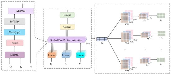
Figure 9. Structure of the multi-attention mechanism.

2.3.4. Classification Stage

After the processing of the above three modules, the output of the multi-attention mechanism is obtained: $Z^{multi}=[z_1^{multi},z_2^{multi},\cdots ,z_n^{multi}]$, where $z_t^{multi}\in {ℝ}^{d_{out}}$ denotes the feature vector at the $t$th time step.

In order to map the output of the multi-attention mechanism to the classification space, this study introduces a fully connected layer (also known as a linear layer). Let the weight matrix of the fully connected layer be $W^c\in {ℝ}^{d_{out}\times C}$, and let the bias vector be $b^c\in {ℝ}^C$, where $C$ is the number of categories of rice phenomics entities. With the fully connected layer, the output $Z^{multi}$ of the multi-attention mechanism can be converted into an un-normalised score vector $S$:

$$S=Z^{multi}{W}^c+b^c$$

(39)

where $S\in {ℝ}^{n\times C}$ and $S_{ij}$ denotes the un-normalised score of time step $i$ corresponding to category $j$. In order to obtain the probability distribution of each category, we use the Softmax function to process the output of the fully connected layer.

In order to obtain the probability distribution of each category, we use the Softmax function to normalise the output of the fully connected layer $S$. The Softmax function is defined as follows:

$$\mathrm{Softmax}(S_{ij})={\displaystyle \frac{\exp (S_{ij})}{{\displaystyle \sum _{k=1}^C\exp }(S_{ik})}}$$

(40)

where $i=1,2,\cdots ,n$ denotes the time step and $j=1,2,\cdots ,C$ denotes the category. After processing using the Softmax function, we obtain a probability matrix $P\in {ℝ}^{n\times C}$, where $P_{ij}$ denotes the probability that the first time step corresponds to the $i$th category.

Finally, the classification decision is made based on the probability matrix $P$. For each time step $i$, the category with the highest probability was selected as the rice phenomics entity category corresponding to that time step:

$${\widehat{y}}_i=\arg {\max }_{j=1}^C{P}_{ij}$$

(41)

where ${\widehat{y}}_i$ denotes the prediction category at the $i$th time step.

2.3.5. Experimental Environment and Parameter Settings

The labelled dataset for this experiment is divided into the training set and the test set according to train_test_split in a 7:3 ratio. The training set is 70%, and the test set is 30%. And the stratified sampling is set by the stratify = y parameter of the train_test_split function to ensure that the proportions of each category in the training and test sets are consistent with the original dataset. The environment is the Windows 10 operating system, the Tensorflow2.10.0 framework, and python3.8, and the plotting uses matplotlib.

Since the setting of hyperparameters plays a crucial and decisive influence on the model’s performance, the parameter settings of the experimental model in this paper are the best results obtained after many optimisation adjustments in the experiments, as shown in Table 4.

Table 4. Experimental parameters.

Parameters	Value
max_length	200
dropout	0.4
learning_rate	0.0001
epoch	50
batchsize	128
embedding loss function	320 Focal Loss

Table 4. Experimental parameters.

Parameters	Value
max_length	200
dropout	0.4
learning_rate	0.0001
epoch	50
batchsize	128
embedding loss function	320 Focal Loss

3. Experiments Results and Discussion

3.1. Evaluation Protocols

To evaluate the performance of the algorithms, various metrics are used. The comparison of the experiments demonstrates that the method proposed in this research produces superior outcomes. The confusion matrix serves as our foundation for the most part. The computing requirements for a classifier to classify a batch of samples from several classes can be expressed in the confusion matrix. True positives, false positives, true negatives, and false negatives are the four parameters, as shown in Table 5.

Table 5. Confusion matrix.

Confusion Matrix		Predicted
		Positive	Negative
True	Positive	TP	FN
	Negative	FP	TN

Table 5. Confusion matrix.

Confusion Matrix		Predicted
		Positive	Negative
True	Positive	TP	FN
	Negative	FP	TN

Accuracy (ACC), precision (Macro-P), recall (Macro-R), the F1-score (Macro-F1-Score), and the area under the curve (Macro-AUC) are the evaluation metrics utilised in this multiclass classification task. For every category of $m$, the confusion matrix has four values: $F{P}_m$ and $F{N}_m$. In contrast, $F{P}_m$ indicates wrongly anticipating the true classification as not $m$, when it is actually classification $m$. $T{P}_m$ indicates accurately predicting the true classification $m$ as classification $m$. Below is the expression for each evaluation metric.

$$ACC={\displaystyle \frac{{\displaystyle \sum _{m=1}^{n=6}T{P}_m}}{{\displaystyle \sum _{m=1}^{n=6}\left(T{P}_m+F{P}_m\right)}}}$$

(42)

$$Macro\text{-P}={\displaystyle \frac{1}{n}}{\displaystyle \sum _{m=1}^{n=6}\left(\frac{T{P}_m}{T{P}_m+F{P}_m}\right)}$$

(43)

$$M\mathrm{acro}\text{-R}={\displaystyle \frac{1}{\mathrm{n}}}{\displaystyle \sum _{m=1}^{n=6}\left(\frac{T{P}_m}{T{P}_m+F{N}_m}\right)}$$

(44)

$$Macro-F1={\displaystyle \frac{2\cdot Macro\text{-}P\cdot M\mathrm{acro}\text{-R}}{M\mathrm{acro}\text{-P}+\mathrm{Macro}\text{-R}}}$$

(45)

Furthermore, the model is evaluated using the receiver operating characteristic (ROC) curve, which is presented in this study. The ROC curve is a graphical representation, with the false positive rate (FPR = 1 − specificity) on the x-axis and the true positive rate (TPR = sensitivity) on the y-axis. The area under the curve (AUC) of the ROC curve, which ranges from zero to one, can be used to intuitively assess the classifier’s performance. The higher the value, the better the model’s final prediction accuracy.

3.2. Experiments Results

In the context of the rice phenomics entity classification experiment, the model based on Roberta–two-layer BiLSTM-MHA demonstrates remarkable efficacy, as evidenced in Figure 10. The model attains an accuracy of 89.56%, signifying that a substantial proportion, approximately 89.56%, of the predicted outcomes are accurately classified. This observation substantiates the model’s high classification accuracy and its capacity to adeptly discern diverse entities within the domain of rice phenomics.

Figure 10. Experimental results of Roberta–two-layer BiLSTM-MHA.

Figure 10. Experimental results of Roberta–two-layer BiLSTM-MHA.

The recall rate of 86.4% signifies the model’s capacity to accurately identify positive instances, thereby reducing the occurrence of false negatives. The enhanced recall rate underscores the model’s ability to capture a substantial number of genuine positive examples during the detection of rice phenotype-related entities, leading to a reduction in false negatives.

The F1-score, a metric that integrates both accuracy and recall, achieves a score of 87.9%. The F1-score offers a comprehensive evaluation of model performance by balancing accuracy and recall, thereby preventing the bias that can arise from an emphasis on a single indicator. The high F1-score further substantiates the validity and reliability of the model in the task of classifying rice phenomics entities.

(1)

Confusion matrix analysis

The result is shown in the confusion matrix in Figure 11. Based on the analysis of diagonal elements from the confusion matrix, the diagonal elements have larger values. For example, the number of samples in which the class ‘Gene’ is truly ‘Gene’ and correctly predicted as ‘Gene’ reaches 539; the number of correctly predicted samples in the ‘Other’ class is correctly predicted as 386 samples, and the “Phenotype” class is correctly predicted as 288 samples. This indicates that the model has high accuracy in identifying rice phenomics entities in the categories of ‘Gene’, ‘Other’, and ‘Phenotype’ and is able to correctly distinguish most of the samples belonging to these categories.

Figure 11. Confusion matrix for Roberta-two-layer BiLSTM-MHA experiments.

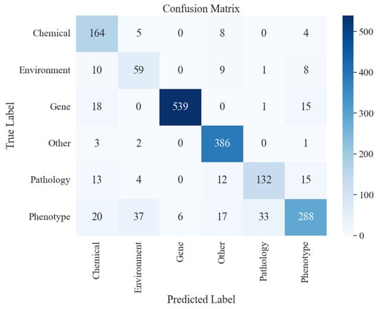
Figure 11. Confusion matrix for Roberta-two-layer BiLSTM-MHA experiments.

Non-diagonal element analysis: in the ‘Chemical’ category, five samples were incorrectly predicted to be in the ‘Environment’ category, and eight samples were incorrectly predicted to be in the ‘Phenotype’ category. In the ‘Environment’ category, 10 samples were incorrectly predicted to be in the ‘Chemical’ category, and 9 samples were incorrectly predicted to be in the ‘Other’ category, and so on. These non-diagonal elements reflect the presence of confusing category pairs in the model. For example, there may be some similarities between the categories ‘Chemical’ and ‘Environment’ and between ‘Environment’ and ‘Other’. Other’ may have some similar features, leading to misclassification by the model.

(2)

ROC curve analysis

From the ROC curve in Figure 12, the curves of each classification are close to the upper left corner. The curve of ‘Class Other’ almost coincides with the upper left corner, and its AUC value reaches 1.0, which indicates that the model has excellent prediction performance in this category, and it can very accurately distinguish the samples of the ‘Other’ category from other categories. The AUC values of ‘Class Chemical’ and ‘Class Gene’ are 0.99, and the AUC values of ‘Class Environment’ and ‘Class Phenotype’ are 0.99, respectively. ‘Class Chemical’ and “Class Gene” have AUC values of 0.99; “Class Environment” and “Class Phenotype” have AUC values of 0.96 and 0.98, respectively, and the macro-average of the model has an AUC value of 0.98. This indicates that the overall model has better classification performance in different classes and is able to maintain a high true rate while ensuring a low false positive rate.

Figure 12. ROC curves for Roberta-two-layer BiLSTM-MHA experiments.

Figure 12. ROC curves for Roberta-two-layer BiLSTM-MHA experiments.

(3)

Model training time and loss analysis

The loss change curves as well as the time curves are shown in Figure 13. In the experiment of rice phenomics entity classification, at the early stage, the loss value decreases rapidly from about 8.7564352 and stabilises around the 22nd round, which indicates that the model can learn and converge quickly, and at the later stage, the loss value also decreases rapidly to around 0.01 and converges. This indicates that the model can effectively learn relevant entity features and has a good entity classification ability. The training time increases with epoch to nearly 3700 s.

Figure 13. Plot of model training rounds versus time and loss.

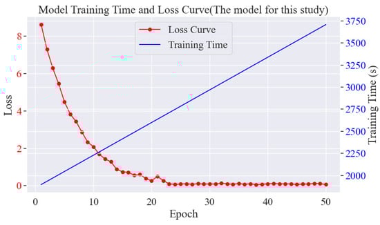
Figure 13. Plot of model training rounds versus time and loss.

3.2.1. Comparison with Traditional Classification Models

In order to comprehensively evaluate the efficacy of Roberta–two-layer BiLSTM–multiple-attention mechanism-based models for classifying entities in rice phenomics, this study carefully selected three representative models, namely logistic regression, a support vector machine (SVM), and Naive Bayes.

The selection of these models was driven by their status as highly representative of traditional machine learning algorithms. The experimental setup entailed the training and testing of all models on an identical rice phenotype dataset, a methodological choice that ensured the consistency of the experimental environment and the reliability and fairness of the experimental results. The findings from these experiments are presented in Table 6.

In terms of accuracy, the support vector machine (SVM) demonstrates superior performance in comparison to traditional classification models; however, its accuracy is only 72.3%. Logistic regression and plain Bayes exhibit even lower accuracy. This is attributable to the fact that the majority of traditional classification models are constructed based on simple statistical assumptions and linear classification boundaries. For instance, logistic regression essentially classifies samples using linear functions, making it difficult to accurately capture the complex nonlinear relationships that exist in abundance in rice phenomics data. The phenotypic features of rice, such as plant height, leaf colour, spike shape, etc., are often interrelated and affected by a variety of factors, such as environmental and genetic factors, etc. Logistic regression is unable to effectively deal with these complex interactions of features, resulting in frequent errors in determining the entity category.

Table 6. Experimental results comparing traditional classification models.

Model	Accuracy	Recall	F1-Score
Logistic regression	68.5%	63.2%	65.7%
Support vector machine	72.3%	68.9%	70.5%
Naive Bayes	65.8%	60.5%	63.0%
Roberta–two-layer BiLSTM-MHA	89.56%	86.4%	87.9%

Table 6. Experimental results comparing traditional classification models.

Model	Accuracy	Recall	F1-Score
Logistic regression	68.5%	63.2%	65.7%
Support vector machine	72.3%	68.9%	70.5%
Naive Bayes	65.8%	60.5%	63.0%
Roberta–two-layer BiLSTM-MHA	89.56%	86.4%	87.9%

In terms of recall, the performance of traditional models is also unsatisfactory. The recall rate of logistic regression is 63.2%; that of plain Bayes is 60.5%, and that of the support vector machine is relatively high, but it is only 68.9%. This clearly shows that the traditional model is prone to miss a large number of real samples in the actual process of rice phenotypic entity identification. Taking the recognition of rice phenotypic entities at specific growth stages as an example, due to the insufficient depth of feature mining in traditional models, some entities with subtle feature differences, such as the yellowing phenotype of leaves caused by different degrees of pigment deficiency, are easily overlooked.

The F1-score, which is a combination of accuracy and recall, highlights the excellence of the Roberta–two-layer BiLSTM-MHA model. The F1-score of this model is 87.9%, which is much higher than that of traditional classification models, proving its leading position in terms of comprehensive performance and its ability to perform the task of classifying rice phenomics entities more efficiently and accurately.

3.2.2. Comparison with Other Deep Learning Models

In addition to comparing with traditional classification models, this study also compares with other common deep learning models based on the Roberta–two-layer BiLSTM-MHA model, which include simple convolutional neural networks (CNNs), recurrent neural networks (RNNs), and BERT models based on the Transformer architecture. All models were trained and tested in the same experimental environment to ensure the scientific validity of the comparison results. The performance comparison of the models is shown in Table 7.

Table 7. Comparison with other deep learning models.

Model	Accuracy	Recall	F1-Score
CNN	75.4%	70.1%	72.6%
RNN	78.2%	73.5%	75.8%
BERT	81.3%	78.6%	79.9%
Roberta–two-layer BiLSTM-MHA	89.56%	86.4%	87.9%

Table 7. Comparison with other deep learning models.

Model	Accuracy	Recall	F1-Score
CNN	75.4%	70.1%	72.6%
RNN	78.2%	73.5%	75.8%
BERT	81.3%	78.6%	79.9%
Roberta–two-layer BiLSTM-MHA	89.56%	86.4%	87.9%

From the loss curves of the different models shown in Figure 14, the loss values of each model are high at the beginning and then decrease rapidly as the epoch progresses. In this study, the model decreases slowly in the early stage and accelerates in the middle and late stages, while the CNN, RNN, and BERT converge slightly slower, and the final loss is slightly higher. This suggests that the model in this study has better fitting and generalisation ability in classifying rice phenomics entities.

Figure 14. Comparison of curve diagrams of different models.

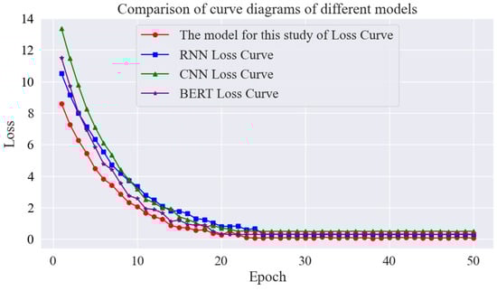
Figure 14. Comparison of curve diagrams of different models.

The experimental results presented in Table 7 are analysed as follows: The CNN model demonstrates significant advantages in the processing of image-based data. However, in the context of rice phenomics entity classification, the model achieves an accuracy of 75.4%, a recall of 70.1%, and an F1-score of 72.6%. This suboptimal performance can be primarily attributed to the fact that CNNs are initially designed to extract local spatial features of an image and capture edges, textures, and other information by sliding a convolutional kernel over the image. However, the rice phenotypic data are mostly presented in text form, and the data features are not the spatial structure of the image, so it is difficult for the CNN to extract effective semantic features from them, which leads to a great limitation of classification performance.

The RNN model has been shown to be advantageous in the processing of sequential data and is capable of capturing the forward and backward dependencies of the data. However, in this experiment, the accuracy was found to be 78.2%; the recall was 73.5%, and the F1-score was 75.8%. While the RNN model has been shown to be capable of modelling the sequence information of rice phenotypic data, it is evident that there are limitations in its learning ability for complex rice phenotypic features, such as those involving multi-factor interactions. Furthermore, it has been observed that the RNN model is prone to the problem of gradient disappearance or gradient explosion with increasing sequence length, which has a significant impact on the model’s training effect.

The BERT model, an archetypal exemplar of the Transformer architecture, has seen extensive deployment in the domain of natural language processing (NLP). In the present experiment, the BERT model demonstrated an accuracy of 81.3%, a recall of 78.6%, and an F1-score of 79.9%. In comparison with the BERT model, the Roberta-based two-layer BiLSTM-MHA model exhibited substantial enhancements in accuracy, recall, and the F1-score. These enhancements are primarily attributable to the two-layer BiLSTM’s capacity to model sequences in both forward and backward directions, thereby comprehensively exploring bi-directional sequence features. In contrast, the multi-attention mechanism facilitates parallel focus on diverse input sequences and the weighting of different feature dimensions, enabling more effective learning of complex patterns in rice phenotypic data.

In summary, the Roberta–two-layer BiLSTM-MHA-based model demonstrates superior performance in the rice phenomics entity classification task, both in comparison with traditional classification models and other deep learning models.

3.2.3. Analysis of the Contribution of the Components of the Model

(1)

Analysis of the validity of Roberta’s pre-training model

In the domain of natural language processing, pre-training models have been identified as a pivotal component in enhancing the efficacy of subsequent downstream tasks. In the context of rice phenomics entity classification, this study aims to provide a comparative analysis of the performance of a Roberta pre-trained model, a BERT pre-trained model, and a model that has not undergone any pre-training. The experimental setup and the specific data are presented in Table 8.

The experimental results indicate that the combination of the pre-trained model of Roberta performs optimally in all indicators. Roberta has acquired extensive semantic and syntactic knowledge in substantial text data through large-scale unsupervised learning. In rice phenotype-related text processing, it is able to profoundly understand the semantics and accurately capture subtle features. For example, when judging the phenotype of a rare rice disease, Roberta can quickly identify the key feature words in the text based on the pre-trained knowledge reserve, which provides a high-quality basis for the subsequent processing of BiLSTM and the multi-head attention mechanism.

Table 8. Experimental results of word embedding model effectiveness analysis.

Model	Accuracy	Recall	F1-Score
Roberta–two-layer BiLSTM-MHA	89.56%	86.4%	87.9%
BERT–two-layer BiLSTM-MHA	81.3%	78.6%	79.9%
two-layer BiLSTM-MHA	72.8%	70.1%	70.5%

Table 8. Experimental results of word embedding model effectiveness analysis.

Model	Accuracy	Recall	F1-Score
Roberta–two-layer BiLSTM-MHA	89.56%	86.4%	87.9%
BERT–two-layer BiLSTM-MHA	81.3%	78.6%	79.9%
two-layer BiLSTM-MHA	72.8%	70.1%	70.5%

As a classic pre-trained model, BERT performs well in natural language processing tasks. However, in the specific domain of rice phenotyping, its ability to learn domain-specific knowledge is slightly weaker than Roberta. When dealing with the complex text associated with rice genes and phenotypes, BERT’s understanding of some terminology and domain-specific expressions is not deep enough, resulting in some misclassifications during the classification process and inferior performance to the Roberta-based model.

The two-layer BiLSTM-MHA, which does not use a pre-trained model, can only rely on the subsequent components to extract simple features from the original text. In the face of the complex semantic information of rice phenotypes, due to the lack of in-depth understanding of the semantics, the key features cannot be effectively extracted, resulting in a significant decline in classification performance, and the accuracy, recall, and F1-scores are much lower than those of the pre-trained model.

(2)

Two-layer BiLSTM Effectiveness Analysis

When processing sequence data, BiLSTM can model the sequence from both forward and reverse directions, fully exploiting bidirectional sequence features. In order to determine the optimal number of BiLSTM layers, we carried out comparative experiments with different numbers of layers, and the specific data are shown in Table 9.

One-layer BiLSTM is able to learn certain contextual dependencies and has some extraction ability for simple rice phenotypic sequence features. However, in the face of complex rice phenotypic semantics, such as those involving phenotypic features under the influence of multiple environmental factors, its feature extraction capability is limited, and it cannot fully mine the key information in the sequences, resulting in relatively low performance.

Table 9. Bilayer BiLSTM as well as BiLSTM layer effect analysis.

BiLSTM Layer	Accuracy	Recall	F1-Score
One layer	80.2%	77.5%	78.5%
Two-layer	89.56%	86.4%	87.9%
Three-layer	85.6%	83.2%	83.7%

Table 9. Bilayer BiLSTM as well as BiLSTM layer effect analysis.

BiLSTM Layer	Accuracy	Recall	F1-Score
One layer	80.2%	77.5%	78.5%
Two-layer	89.56%	86.4%	87.9%
Three-layer	85.6%	83.2%	83.7%

On the basis of one layer, two-layer BiLSTM further deepens the mining of contextual information. It can learn more advanced semantic features, such as complex associations between different rice phenotypes. When analysing the relationship between the rice growth cycle and phenotypic changes, two-layer BiLSTM is able to better capture the feature changes on the time series and significantly improve the classification performance of the model.

The characteristics of the three-layer BiLSTM model can be seen from the curves in Figure 15. Although the three-layer BiLSTM has the theoretical potential to learn more complex features, in terms of the actual training process, the overfitting problem is more prominent due to the large number of layers of the network it comes with, as well as the fact that it is again fused with other models (Roberta and the multi-head attention mechanism).

As shown in Figure 15a, in the pre-training period, the accuracy of the training set of the three-layer BiLSTM rises rapidly, while the accuracy of the test set begins to decline after reaching a certain level. This indicates that the model overcaptures the noise in the training data during the training process and overlearns the training data, which leads to the weakening of the model’s generalisation ability on new data such as the test set, which then leads to the difficulty of continuing to improve the accuracy of the test set or even a decline, so the overall performance of the model will also be affected. Looking at Figure 15b, in terms of the loss curve, the initial loss of the three-layer BiLSTM model is high and decreases quickly in the first 15 rounds, but after 15 rounds, the loss rises and fluctuates greatly due to the start of overfitting. Compared to the one-layer and two-layer models, their final loss values begin to show an upward fluctuating trend. As for the training time, it can be clearly seen from the three training time curves that the training time curve of the three-layer BiLSTM is located at the top, and with the increase in the number of training rounds, the required training time is significantly more than that of the one-layer and two-layer models.

Figure 15. Comparison of the effect of the number of layers of BiLSTM models on the training time, loss, and accuracy. (a) Variation in accuracy between the test and training sets of three-layer BiLSTM; (b) Variation in BiLSTM loss and consumption time for different number of layers.

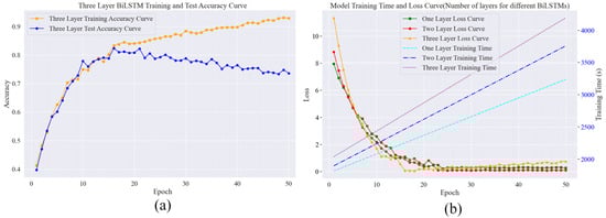
Figure 15. Comparison of the effect of the number of layers of BiLSTM models on the training time, loss, and accuracy. (a) Variation in accuracy between the test and training sets of three-layer BiLSTM; (b) Variation in BiLSTM loss and consumption time for different number of layers.

(3)

Impact of Multi-head Attention Mechanisms

The multi-head attention mechanism plays a key role in improving the model’s ability to learn complex data patterns. It achieves a more comprehensive and deeper understanding of the data by focusing on different parts of the input sequence in parallel and assigning weights to different feature dimensions. In order to explore the specific impact of the multi-head attention mechanism in depth, this study conducted comparative experiments with and without the multi-head attention mechanism as well as with different numbers of heads (2, 4, 8, and 16), as shown in Table 10.

When the model lacks the multi-head attention mechanism, it can only rely on BiLSTM to extract features according to a fixed pattern. When facing the complex semantic and feature relationships in the rice phenotypic data, it is not possible to strengthen and filter the important features in a targeted way, resulting in the insufficient mining of key information by the model and a significant decline in classification performance.

Table 10. Results of the analysis of the effectiveness of the multi-attention mechanism.

Model	Accuracy	Recall	F1-Score
Roberta–two-layer BiLSTM	82.1%	80.3%	80.3%
Roberta–two-layer BiLSTM-MHA (2 heads)	84.3%	82.5%	82.5%
Roberta–two-layer BiLSTM-MHA (4 heads)	86.7%	85.1%	85.1%
Roberta–two-layer BiLSTM-MHA (8 heads)	89.56%	86.4%	87.9%
Roberta–two-layer BiLSTM-MHA (16 heads)	85.3%	84.6%	84.7%

Table 10. Results of the analysis of the effectiveness of the multi-attention mechanism.

Model	Accuracy	Recall	F1-Score
Roberta–two-layer BiLSTM	82.1%	80.3%	80.3%
Roberta–two-layer BiLSTM-MHA (2 heads)	84.3%	82.5%	82.5%
Roberta–two-layer BiLSTM-MHA (4 heads)	86.7%	85.1%	85.1%
Roberta–two-layer BiLSTM-MHA (8 heads)	89.56%	86.4%	87.9%
Roberta–two-layer BiLSTM-MHA (16 heads)	85.3%	84.6%	84.7%

When the multi-head attention mechanism is set to two heads, although the model can pay attention to some features in parallel, due to the limited number of heads, the dimension of attention to features is not broad enough. When dealing with rice phenotypic data, only some more obvious key features can be captured, and it is difficult to effectively identify those features hidden in complex semantics and data relationships. This makes the model show some limitations when facing the task of complex phenotype classification, and the performance indexes have obvious gaps compared to those of models with higher head counts.

As the number of heads increased to four, the model’s ability to learn features improved. It is able to pay attention to relevant information in rice phenotypic data from multiple perspectives; for example, when analysing the association between rice pests and diseases and phenotypes, it is able to capture more feature relationships at different levels, which makes the accuracy, recall, and F1-score of the model improve to a certain extent. The model achieves the best balance of performance when set to the 8-head multi-head attention mechanism.

It can pay attention to the input sequences in parallel from a richer perspective; comprehensively capture multiple features such as morphology, colour, growth environment, etc., in the rice phenotypic data; and effectively learn the relationship between these complex features through weighted integration. This makes the model perform well in various performance indicators, finding a better balance between feature diversity and computational resource consumption and achieving high classification performance with relatively reasonable computational resource consumption.

When the multi-head attention mechanism is set to 16 heads, due to the excessive number of heads, the dimension of information that the model needs to process increases dramatically, resulting in a sharp increase in computational resource consumption. The excessive number of heads also makes the model susceptible to some noise information during the training process, which affects the generalisation ability of the model to a certain extent, leading to a decrease in the accuracy and F1-score compared to the eight-head scenario.

(4)

Analysis of the effectiveness of different loss functions

This experiment aims to explore the effectiveness of different loss functions on the model. It was analysed, respectively, using the cross-entropy loss, focal loss, and label smoothing loss functions for experimental comparison. The experimental results are shown in Table 11. As well as loss, consumed time and F1-score variations with epoch are shown in Figure 16.

Table 11. Evaluation metrics for different loss functions.

Loss Function	Accuracy	Recall	F1-Score
Cross-entropy loss function	87.1%	85.6%	86.7%
Focus loss function	89.56%	86.4%	87.9%
Label smoothing loss function	86.7%	85.2%	86.2%

Table 11. Evaluation metrics for different loss functions.

Loss Function	Accuracy	Recall	F1-Score
Cross-entropy loss function	87.1%	85.6%	86.7%
Focus loss function	89.56%	86.4%	87.9%
Label smoothing loss function	86.7%	85.2%	86.2%

Figure 16. Comparison of loss, the F1-score, and the elapsed time for different loss functions. (a) Variation in loss and consumption time for different loss functions; (b) Variation in F1-score with different loss functions.

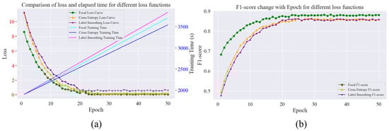
Figure 16. Comparison of loss, the F1-score, and the elapsed time for different loss functions. (a) Variation in loss and consumption time for different loss functions; (b) Variation in F1-score with different loss functions.

From Figure 16a, it can be seen that the loss values of the three loss functions are higher at the beginning of training but start to decline with the increase in training rounds; the focus loss function and the cross-entropy loss function decline faster than the label smoothing loss function; the focus loss function tends to stabilise after about 22 rounds, and the cross-entropy loss function tends to stabilise after about 25 rounds. The label smoothing loss function decreases slowly in the early stage and stabilises at a slightly higher value near 0.5 in the late stage; in terms of the time consumed for training, the label smoothing loss function is the longest, and the cross-entropy loss function is the shortest. From the F1-score change in Figure 16b, the initial value of the F1-score using focus loss is higher, near 0.68, and as the number of rounds increases, the F1-score also starts to rise. In terms of the evaluation indexes shown in Table 11, the accuracy, recall, and F1-scores of the focal loss function are 89.56%, 86.4%, and 87.9%, respectively, which are the best performers in terms of the three loss functions in this study, and the label smoothing loss function is relatively weak, with an accuracy rate of 86.7%, a recall rate of 85.2%, and an F1-score of 86.2%. The reason is that the focus loss function learns by focusing on difficult samples, which has obvious advantages in dealing with problems such as data imbalance; the label smoothing loss function is time-consuming to train, and the evaluation indexes are not outstanding, but it can smooth the labels to prevent overfitting.

3.3. Discussion

In Roberta–two-layer BiLSTM-MHA-based rice phenomics entity classification experiments, parameter settings have a key impact on model performance. In this section, this study will explore in detail the performance of the model in terms of accuracy, recall, and the F1-score for different values of the learning rate (lr), random inactivation rate (dropout), batch size, and optimiser in order to determine the optimal parameter combinations and analyse their effectiveness.

(1)

The influence of the learning rate (lr)

The learning rate, a pivotal hyperparameter in the model training process, directly influences the step size of the model during parameter updating. In essence, the learning rate modulates the pace of the model along the gradient of the loss function during the optimisation process. During the training process of the deep learning model, the model calculates the gradient of the loss function to the parameters through the back-propagation algorithm and then updates the parameters according to the learning rate. This process gradually reduces the value of the loss function and makes the model’s prediction results closer to the real value. In this study, a series of different learning rates were setup for the experiment, and the results are shown in Figure 17.

When the learning rate is set too small, such as 0.00001 and 0.00005 in the experiments, the model changes the parameters by an extremely small amount during each parameter update. This means that the model moves very slowly in the space of the loss function and requires a large number of training iterations to gradually approach the optimal solution. In practice, this leads to a significant increase in training time and resource consumption. Concurrently, the gradual nature of parameter updates hinders the model’s capacity to fully grasp the intricate characteristics and patterns embedded within the data, consequently leading to suboptimal performance metrics such as accuracy, recall, and the F1-score. To illustrate this point, consider the rice phenomics entity classification task. In this scenario, the model might encounter challenges in accurately discerning the subtle phenotypic variations influenced by distinct growth stages and environmental factors in rice, resulting in an increased number of misclassifications.

Figure 17. Impact of the learning rate on model performance.

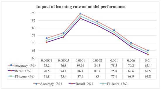
Figure 17. Impact of the learning rate on model performance.

On the contrary, when the learning rate is set too large, e.g., 0.006 and 0.01, the step size of the model during parameter update is too large. This makes the model skip the optimal solution in the loss function space or even oscillate violently around the optimal solution and fail to converge stably. In this case, the training process of the model becomes unstable, and the value of the loss function fails to decrease consistently and may even rise. This results in the model failing to learn effective features, leading to a significant drop in various performance metrics. For example, in the experiment, the model may have a great deviation in the classification of some samples, incorrectly classifying samples originally belonging to a certain phenotype category to other categories, which seriously affects the classification accuracy of the model.

The learning rate of 0.0001, on the other hand, showed the best results in this experiment. This value allows the model to maintain a certain update speed when the parameters are updated without missing the optimal solution because of the large step size. The model is able to converge to a better state in a relatively short period of time and fully learn the features and laws in the rice phenotypic data. In practice, this means that the model is able to accurately identify various phenotypic entities of rice, regardless of whether they are common phenotypes or special phenotypes with subtle differences, thus providing reliable support for the study of rice phenomics.

(2)

Impact of dropout

The random deactivation rate (dropout) is a widely used regularisation technique in deep learning, the core principle of which is to randomly ‘dropout’ some of the neurons and their connections in the neural network with a certain probability during the model training process. This operation breaks the complex co-adaptation between neurons, so the model cannot overly rely on some specific neuron connection patterns, thus improving the generalisation ability of the model and effectively preventing the occurrence of the overfitting phenomenon. The experimental results for different dropout values are plotted in Figure 18.

From Figure 18, we can see that when the dropout value is small, such as 0.2 in the experiment, the model discards fewer neurons during the training process, and most of the connections between neurons are preserved. This makes it easy for the model to learn some detailed features, or even noisy information, in the training data, thus exhibiting higher accuracy on the training set. However, this over-learning of the training data leads to the model being unable to accurately recognise new sample patterns when faced with the test set, and overfitting occurs, resulting in a decrease in accuracy, recall, and the F1-score on the test set. For example, in the rice phenomics entity classification task, the model may remember the special phenotypic features of some rice samples in the training set, but these features are not universal, and when it encounters rice samples with different growing environments or other disturbing factors in the test set, the model will make classification errors.

Figure 18. Experimental results for different dropout values.

Figure 18. Experimental results for different dropout values.

With the gradual increase in the dropout value, the number of neurons discarded by the model increases; the co-adaptation between neurons is effectively suppressed, and the overfitting phenomenon is alleviated. In the experiment, when the dropout value is 0.3, the performance of the model on the test set is improved, and all the indexes are improved. This indicates that a moderate increase in the dropout value helps the model learn more general features and enhances the generalisation ability of the model.

However, when the dropout values are too large, such as 0.6 and 0.7, the model discards too many neurons during the training process, resulting in a serious impact on the model’s learning ability. The model cannot fully learn the effective features in the data, and the underfitting phenomenon occurs. At this time, the accuracy, recall, and F1-score of the model on both the training and test sets are significantly reduced. For example, when classifying rice phenotypes, the model may not be able to accurately capture some key phenotypic features, incorrectly classify rice samples of different phenotypes into the same category, or fail to identify samples of some special phenotypes, resulting in a significant increase in the classification error rate.

In this experiment, the dropout value of 0.4 showed the best effect. This value finds a good balance between preventing overfitting and maintaining the learning ability of the model. It can effectively inhibit the co-adaptation between neurons to avoid the model over-learning the noisy information in the training data but also ensure that the model has enough neuron connections to learn the effective features in the data.

(3)

Influence of batch size

Batch size refers to the number of samples input into the model during each training, which plays a pivotal role in the model training process and has a significant impact on the training efficiency, stability, and final model performance. In this study, batch sizes of 8, 16, 64, 128, 256, and 512 were selected for a series of experiments, and the experimental results are shown in Figure 19.

Figure 19. Experimental results of the effect of different batch size values on the performance of the model.

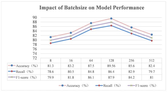
Figure 19. Experimental results of the effect of different batch size values on the performance of the model.

As demonstrated in Figure 18, when the batch size is set to a small value, such as 8 or 16, as was the case in the experiments, there is a limited number of samples on which each model parameter update is based. This results in large fluctuations in the estimate of the gradient when calculating the gradient due to the limitations of the samples, leading to unstable parameter updates. This phenomenon can be likened to an attempt to locate the optimal solution within a confined space, where local deviations can easily lead to a loss of direction. This instability in the parameter update process hinders the model’s ability to capture global features in the data, consequently impairing its generalisation capabilities. In the rice phenomics entity classification task, the model may not accurately identify phenotypic features that exhibit subtle differences under varying growth environments and developmental stages, consequently leading to suboptimal accuracy, recall, and F1-score metrics. Additionally, due to the limited number of samples processed in each iteration, the model requires extensive training, which will considerably extend the training time and reduce the training efficiency.

However, as the batch size increases, the situation improves. When the batch size is 64, each parameter update is based on more samples; the gradient is estimated more accurately, and the stability of the parameter update is significantly improved. The model is able to learn from more data features, which improves the performance of the model to a certain extent, and all the indexes have increased. Consequently, the model exhibits enhanced stability in its progression towards the optimal solution during the training process, and the learning of rice phenotypic features is characterised by greater comprehensiveness and depth.

However, when the batch sizes are set too high (for example, 256 and 512), the model is more likely to find a local optimal solution, although the stability of parameter updating is enhanced. This is because when the data volume is high, the model is more likely to be attracted by the local optimal solution during the optimisation process, and it is difficult to find the global optimal solution. To illustrate this point, consider the rice phenotypic classification model. It has been observed that the model may become overly reliant on certain common phenotypic feature patterns, thereby overlooking unique cases or subtle feature distinctions. This can result in a decline in the model’s classification capability and a decrease in accuracy, recall, and the F1-score when confronted with diverse test samples. Moreover, the utilisation of overly large batch sizes can impose challenges related to computational resources, necessitating greater memory to store and process data. This can potentially become a constraining factor in scenarios where hardware resources are limited.

In this experiment, a batch size of 128 was determined to be an optimal balance between training efficiency, stability, and model performance. This ensured that there were sufficient samples to support each parameter update, thereby enhancing the accuracy of gradient estimation and ensuring the stability of parameter updates. Additionally, this approach prevented the problem of falling into a local optimal solution due to a large batch size. The model consumes reasonable computational resources, facilitating the comprehensive learning of various features in rice phenotyping data. This results in optimal performance metrics, including accuracy, recall, and the F1-score, thereby ensuring the reliable classification of rice phenomics entities.

(4)

Optimiser Impact

Optimizers take on the key responsibility of tuning model parameters to minimise the loss function in deep learning model training, and the characteristics and strategies of different optimizers can significantly affect the training process and final performance of the model. In this study, SGD, Adam, and Adagrad are selected to conduct experiments, and the experimental results are shown in Figure 20.

Figure 20. Results of the impact of different optimisers on the performance of the model.

Figure 20. Results of the impact of different optimisers on the performance of the model.

Stochastic gradient descent (SGD) is a fundamental optimiser that calculates the gradient based on a small batch of samples randomly selected in each iteration, thereby updating the model parameters. In principle, SGD considers only the gradient information of the current small batch of samples in each parameter update, a method that is computationally simple and efficient. However, this approach is inherently limited. The random selection of samples for updating purposes introduces significant noise during gradient estimation, resulting in unstable parameter updates and frequent oscillations during the training process. In the rice phenomics entity classification experiment, the SGD optimiser demonstrates instability in the loss function value of the model during training, hindering the ability to decrease steadily. This hinders the model’s ability to converge on a more optimal solution, as evidenced by the experimental findings, which demonstrate an accuracy of 75.6%, a recall of 72.9%, and an F1-score of 74.2%. In the context of rice phenomics entity classification, the model frequently misidentifies similar phenotypic entities, leading to an inaccurate classification. This issue significantly impacts the practical application of the model.

Adagrad (Adaptive gradient descent) is an optimiser that improves SGD (stochastic gradient descent) by adaptively adjusting the learning rate of each parameter. This is based on the cumulative sum of the squares of the gradients of each parameter in previous iterations, with the learning rate of frequently updated parameters being decreased and the learning rate of less frequently updated parameters being increased. This adaptive adjustment of the learning rate renders the model more reasonable for updating parameters during the training process, thereby enhancing its stability to a certain extent. However, Adagrad is not without its drawbacks. It is notable that Adagrad constantly accumulates the square of the gradient during the calculation process, resulting in a decay of the learning rate with training, which can lead to an insufficient learning rate at a later stage and a slower convergence of the model. In this experiment, while Adagrad exhibited relative stability during training and did not demonstrate violent oscillations as observed in SGD, its convergence speed was notably slower. The resulting model demonstrated an accuracy of 82.5%, a recall of 79.8%, and an F1-score of 81.1%, all of which were lower than the performance of the optimal optimiser. This suggests that, in practice, the model requires a greater investment of time to achieve a satisfactory level of performance, and its classification performance is still inferior to that of other optimisers of a higher calibre.

The Adam (adaptive moment estimation) optimiser synthesises the merits of Adagrad and RMSProp in that it not only adaptively adjusts the learning rate for each parameter but also employs momentum to accelerate convergence. Adam considers both the first-order moments of the gradient (the mean) and the second-order moments of the gradient (the uncentered variance) when calculating the gradient and dynamically adjusts the learning rate through the estimation of these two moments. In the rice phenomics entity classification experiments, the Adam optimiser demonstrated excellent performance, exhibiting a rapid convergence rate and the capacity to swiftly reduce the loss function value at the commencement of the training period, thereby enabling the model to expeditiously approach the optimal solution. Concurrently, the Adam optimiser exhibited remarkable stability during the training process, with the loss function value diminishing in a smooth and continuous manner, thus circumventing the oscillation problem engendered by the unstable gradient. The model utilising the Adam optimiser attains 89.56% in accuracy, 86.4% in recall, and 87.9% in the F1-score, thereby demonstrating superiority over the SGD and Adagrad optimisers across all performance metrics. This facilitates the accurate identification of a range of phenotypic features during the classification of rice phenotypic entities, encompassing both prevalent phenotypes and distinctive ones with nuanced variations. The high-precision classification it enables provides substantial support for the study of rice phenomics.

(5)

Exploration of the possibility of using the model for phenotyping other objects

From the perspective of the model architecture itself, the Roberta-based two-layer BiLSTM-MHA model has efficient text feature extraction and semantic understanding capabilities. In the rice phenotype classification task, it can effectively extract the semantic features of the rice phenomics text and realise efficient classification. This provides a certain foundation for applying it to the classification of phenotypic entities in other domains. For different types of phenotypes, as long as their phenotypic information can be represented in the form of textual data, the model is theoretically applicable. For example, in the field of botany, the phenotypic characteristics, such as morphology, physiology, and biochemistry, of crops other than rice, such as wheat, can also be recorded through textual descriptions. The model can process these texts and mine the phenotypic information embedded in them. In the field of zoology, animal behavioural characteristics, physiological indicators, and other phenotypic descriptive texts may also be analysed with the help of the model.

However, the use of models for phenotype categorization in other domains requires some additional considerations. First, the phenotypic expertise systems of different domains are quite different, which requires high generalisation ability of the model. The parameters of the current model are derived from training based on rice phenotypic data, and a lot of pre-training and fine-tuning is required for use in other domains. Second, the quality of the data as well as the size of the data volume is also important. Phenotypic classification in other domains may lack sufficient high-quality labelled data, and missing or incomplete data can also lead to biassed predictions of the model in learning semantic features.

3.4. Results and Analysis of Example Analyses

In order to present the performance of the Roberta–two-layer BiLSTM-MHA model in a more intuitive manner, a set of validation data has been selected for analysis in this paper. The prediction results of the model on the entities therein are demonstrated through specific examples, the details of which are shown in Figure 21. The heat map labels predicted by the model example in this study are shown in Figure 22.

Figure 21. Predicted results of the instance analysis.

Figure 21. Predicted results of the instance analysis.

By analysing validation data for entity classification in rice phenomics using the Roberta–two-layer bidirectional long- and short-term memory network–multi-head attention (BiLSTM-MHA) model, the following findings were made.

For the entities in the provided rice-related text, when the model processes statements such as “稻瘟病经常会影响到水稻的株高以及分蘖数” (rice blast often affects plant height as well as tiller number in rice)’, it correctly predicts “稻瘟病” (rice blast) as ‘Pathology’ (pathology) and “株高” (plant height) and “分蘖数” (number of tillers) as “phenotype”. In addition, “干旱” (drought) and “高温” (high temperature) were also correctly classified as ‘Environment’ in “在干旱且高温环境下 TaDREB2 基因参与调控小麦的热激蛋白表达” (involvement of the TaDREB2 gene in the regulation of heat stress protein expression in wheat under drought and high temperatures). And as can be seen from Figure 22, by inputting the text “稻瘟病经常会影响到水稻的株高以及分蘖数” (rice blast often affects plant height as well as tiller number in rice), the model predicts the label for each word, and the darker the colour, the higher the probability value of the matching label, and the model can correctly predict the entity.

Figure 22. Example heat map labels predicted by the model examples in this study.

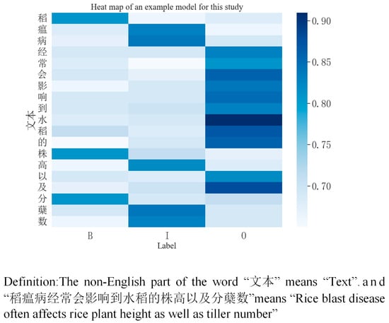
Figure 22. Example heat map labels predicted by the model examples in this study.

However, there are some inaccuracies in the model. For example, in “在干旱且高温环境下 TaDREB2 基因参与调控小麦的热激蛋白表达” (the TaDREB2 gene is involved in the regulation of heat-expressed proteins in wheat under drought and high temperatures), the “TaDREB2 基因” (TaDREB2 gene) is incorrectly predicted to be in the ‘Pathology’ category, whereas it should actually belong to the ‘Gene’ category. In the ‘TaDREB2 gene’ scenario, it was incorrectly predicted to be a ‘Pathology’, whereas it actually belongs to the ‘Gene’ category. In examples such as “稻瘟病经常会影响到水稻的株高以及分蘖数” (rice blast disease often affects rice plant height as well as tiller number), potential prediction errors may occur due to factors similar to the previous situation, such as insufficient training data, poor feature learning, or interference from other entities in the text.

3.5. Generalisation Experiment

In order to validate the generalisation ability of the rice phenomics entity classification model based on Roberta–two-layer BiLSTM-MHA, this study uses the publicly available dataset CLUENER2020 to carry out generalisation experiments.

(1)

Introduction of the dataset

CLUENER2020 contains 10 different categories, namely organisation, name, address, company, government, book, game, movie, position, and scene. As demonstrated in Table 12, this dataset boasts extensive domain coverage and diversity, thus providing an effective means to assess the generalisation performance of the model on diverse entity types.

(2)

Experimental results and analysis

Following the implementation of multiple training and testing cycles, the model’s performance metrics for various categories have been obtained, as illustrated in Figure 22. And the performance evaluation of this research model in the public dataset and the dataset of this research is shown in Table 13.

Table 12. Comparison of model evaluation results between the self-developed dataset and the publicly available dataset CLUENER2020.

Dataset	Accuracy	Recall	F1-Score
Dataset for this study	89.56%	86.4%	87.9%
CLUENER2020	91.38%	90.94%	91.57%

Table 12. Comparison of model evaluation results between the self-developed dataset and the publicly available dataset CLUENER2020.

Dataset	Accuracy	Recall	F1-Score
Dataset for this study	89.56%	86.4%	87.9%
CLUENER2020	91.38%	90.94%	91.57%

As illustrated in Figure 23, for categories comprising a substantial number of samples, such as names, companies, and organisations, the model demonstrates a commendable level of accuracy and an F1-score that is notably high. This observation signifies that the model exhibits an exceptional capacity for recognising prevalent categories. Conversely, for categories with a limited number of samples, such as book titles and movies, the model’s performance exhibits a slight decline, which may be attributable to insufficient data, resulting in inadequate learning by the model within these categories.

Then, from Figure 24, it can be seen that the initial loss value of this model applied on the public dataset is about 9.76645, which decreases rapidly in the first 18 rounds of training, and it tends to stabilise close to 0.01, which indicates that the model can learn the data features quickly in the pre-training period, and reaches a better convergence state in the later period, and the fitting effect is good.

Then, the training time increases linearly with the number of training rounds, increasing to nearly 4300 s, which is an increase in the consumed time compared to the dataset of rice phenomics entity classification in this study, due to the fact that the public dataset has a larger amount of data compared to that of this study, as well as a different level of complexity of the data.

Figure 23. Breakdown of different entity categories in CLUENER2020.

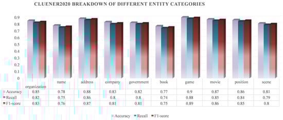
Figure 23. Breakdown of different entity categories in CLUENER2020.

Table 13. Distribution of the training and test sets for the CLUENER2020 dataset.

Datasets	Categories	Quantities	Datasets	Categories	Quantities
training data	address	2829	Testing data	address	364
training data	book	1131	Testing data	book	152
training data	company	2897	Testing data	company	366
training data	game	2325	Testing data	game	287
training data	government	1797	Testing data	government	244
training data	movie	1109	Testing data	movie	150
training data	name	3661	Testing data	name	451
training data	organisation	3075	Testing data	organisation	344
training data	position	3052	Testing data	position	425
training data	scene	1462	Testing data	scene	199

Table 13. Distribution of the training and test sets for the CLUENER2020 dataset.

Datasets	Categories	Quantities	Datasets	Categories	Quantities
training data	address	2829	Testing data	address	364
training data	book	1131	Testing data	book	152
training data	company	2897	Testing data	company	366
training data	game	2325	Testing data	game	287
training data	government	1797	Testing data	government	244
training data	movie	1109	Testing data	movie	150
training data	name	3661	Testing data	name	451
training data	organisation	3075	Testing data	organisation	344
training data	position	3052	Testing data	position	425
training data	scene	1462	Testing data	scene	199

Figure 24. Plot of model training time and loss variation under the public dataset (CLUENER2020).

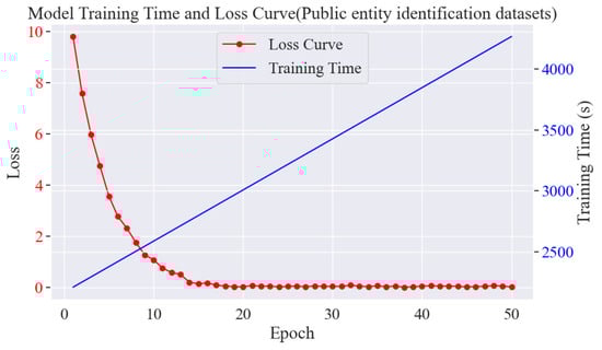
Figure 24. Plot of model training time and loss variation under the public dataset (CLUENER2020).

4. Conclusions

In this paper, we propose a rice phenomics entity classification model based on the Roberta–two-layer BiLSTM-MHA to address the problems of complex feature extraction and the need to improve the classification accuracy of the model for rice phenomics entity classification.

Firstly, the Roberta pre-training model is used to obtain the deep semantic features of rice phenotypes; then, the two-layer BiLSTM is used to further capture the context dependency of the phenotypic features to enhance the feature representation. Next, a multi-head attention mechanism is introduced to enable the model to focus on key phenotypic features.

Then, experiments were conducted on multi-source rice phenotypic datasets, including phenotypic data under different growth stages and environmental conditions. The experimental results verified that the model has higher accuracy, recall, and F1-scores compared to traditional methods and some simple deep learning models in the rice phenomics entity classification task, which effectively improves the classification performance.

In the follow-up work, the authors will consider expanding the dataset to enhance the model’s generalisation ability and explore the integration with computer vision and other technologies to achieve multimodal data-driven rice phenotypic entity classification to provide a more powerful analysis tool for rice phenomics research.

References

- Dharini, P.; Ramesh, N.; Sundari, A.; Thangavel, P. Effect of Biostimulants on the Growth Attributes and Yield of Rice. J. Adv. Biol. Biotechnol. 2024, 27, 697–702. [Google Scholar] [CrossRef]
- de Verdal, H.; Segura, V.; Pot, D.; Salas, N.; Garin, V.; Rakotoson, T.; Raboin, L.-M.; VomBrocke, K.; Dusserre, J.; Pacheco, S.A.C.; et al. Performance of phenomic selection in rice: Effects of population size and genotype-environment interactions on predictive ability. PLoS ONE 2024, 19, e0309502. [Google Scholar] [CrossRef] [PubMed]
- Kikuchi, S.; Bheemanahalli, R.; Jagadish, K.S.; Kumagai, E.; Masuya, Y.; Kuroda, E.; Raghavan, C.; Dingkuhn, M.; Abe, A.; Shimono, H. Genome-wide association mapping for phenotypic plasticity in rice. Plant Cell Environ. 2017, 40, 1565–1575. [Google Scholar] [CrossRef] [PubMed]
- Hearst, M.A.; Dumais, S.T.; Osuna, E.; Platt, J.; Scholkopf, B. Support vector machines. IEEE Intell. Syst. Their Appl. 1998, 13, 18–28. [Google Scholar] [CrossRef]
- van Cutsem, T.; Wehenkel, L.; Pavella, M.; Heilbronn, B.; Goubin, M. Decision tree approaches to voltage security assessment. IEE Proc. C Gener. Transm. Distrib. 1993, 140, 189–198. [Google Scholar] [CrossRef]
- Wang, Y.; Tian, Z.; Zhang, S.; Guan, Y.; Ke, Q.; Yang, H. Flood risk assessment by heterogeneous ensemble learning techniques: A case study of Shenzhen City, China. J. Hydrol. 2025, 650, 132566. [Google Scholar] [CrossRef]
- Han, C.; Luo, Z.; Gu, W.; Chen, J. A Random Walk Tensor Model for Heterogeneous Network Entity Classification. IEEE Access 2019, 7, 72749–72760. [Google Scholar] [CrossRef]
- Dai, H.; Song, Y.; Wang, H. Ultra-Fine Entity Typing with Weak Supervision from a Masked Language Model. arXiv 2021, arXiv:2106.04098. [Google Scholar]
- Ding, N.; Chen, Y.; Han, X.; Xu, G.; Xie, P.; Zheng, H.-T.; Liu, Z.; Li, J.; Kim, H.-G. Prompt-Learning for Fine-Grained Entity Typing. arXiv 2022, arXiv:2108.10604. [Google Scholar]
- Xu, B.; Zhang, Z.; Du, M.; Wang, H.; Song, H.; Xiao, Y. Semi-supervised Learning for Fine-Grained Entity Typing with Mixed Label Smoothing and Pseudo Labeling. In Proceedings of the Database Systems for Advanced Applications, Lecture Notes in Computer Science, Tianjin, China, 17–20 April 2023; pp. 727–736. [Google Scholar] [CrossRef]
- Deng, J.; Liu, J.; Ma, X.; Qin, X.; Jia, Z. Local Feature Enhancement for Nested Entity Recognition Using a Convolutional Block Attention Module. Appl. Sci. 2023, 13, 9200. [Google Scholar] [CrossRef]
- Zhang, H.; Wang, X.; Liu, J.; Zhang, L.; Ji, L. Chinese named entity recognition method for the finance domain based on enhanced features and pretrained language models. Inf. Sci. 2023, 625, 385–400. [Google Scholar] [CrossRef]
- Yuan, T.; Qin, X.; Wei, C. A Chinese Named Entity Recognition Method Based on ERNIE-BiLSTM-CRF for Food Safety Domain. Appl. Sci. 2023, 13, 2849. [Google Scholar] [CrossRef]
- Hu, H.; Cheng, C.; Ye, Q.; Peng, L.; Shen, Y. Enhancing traditional Chinese medicine diagnostics: Integrating ontological knowledge for multi-label symptom entity classification. Math. Biosci. Eng. 2024, 21, 369–391. [Google Scholar] [CrossRef]
- Masaling, N.A.P.; Suhartono, D. Utilizing RoBERTa and XLM-RoBERTa pre-trained model for structured sentiment analysis. Int. J. Inform. Commun. Technol. (IJ-ICT) 2024, 13, 410–421. [Google Scholar] [CrossRef]
- Barnes, J.; Oberlaender, L.; Troiano, E.; Kutuzov, A.; Buchmann, J.; Agerri, R.; Øvrelid, L.; Velldal, E. SemEval 2022 Task 10: Structured Sentiment Analysis. In Proceedings of the 16th International Workshop on Semantic Evaluation (SemEval-2022), Online, 14–15 July 2022; Association for Computational Linguistics: Seattle, WA, USA, 2022; pp. 1280–1295. [Google Scholar] [CrossRef]
- Li, N.; Wang, Y.; Dong, Y.; Qiu, S. Named entity identification method for manufacturing equipment faults based on improved Roberta. J. Phys. Conf. Ser. 2024, 2902, 012017. [Google Scholar] [CrossRef]
- Gao, F.; Zhang, L.; Wang, W.; Zhang, B.; Liu, W.; Zhang, J.; Xie, L. Named Entity Recognition for Equipment Fault Diagnosis Based on RoBERTa-wwm-ext and Deep Learning Integration. Electronics 2024, 13, 3935. [Google Scholar] [CrossRef]
- Devlin, J.; Chang, M.W.; Lee, K.; Toutanova, K. BERT: Pre-training of Deep Bidirectional Transformers for Language Understanding. arXiv 2018, arXiv:1810.04805. [Google Scholar]
- Liu, Y.; Ott, M.; Goyal, N.; Du, J.; Joshi, M.; Chen, D.; Levy, O.; Lewis, M.; Zettlemoyer, L.; Stoyanov, V. RoBERTa: A Robustly Optimized BERT Pretraining Approach. arXiv 2019, arXiv:1907.11692. [Google Scholar]
- Fu, Z.; Wang, Y.; Zhou, L.; Li, K.; Rao, H. Partial Discharge Recognition of Transformers Based on Data Augmentation and CNN-BiLSTM-Attention Mechanism. Electronics 2025, 14, 193. [Google Scholar] [CrossRef]
- Zhao, J.; Liu, N.; Ye, J.; Liu, C.; Sun, F.; Lv, L. CEEMD-FFT-BiLSTM based model for power line loss prediction. J. Phys. Conf. Ser. 2024, 2846, 012003. [Google Scholar] [CrossRef]
- Yang, H.; Yao, L.; Cai, J.; Wang, Y.; Zhao, X. A new interest extraction method based on multi-head attention mechanism for CTR prediction. Knowl. Inf. Syst. 2023, 65, 3337–3352. [Google Scholar] [CrossRef]
Disclaimer/Publisher’s Note: The statements, opinions and data contained in all publications are solely those of the individual author(s) and contributor(s) and not of MDPI and/or the editor(s). MDPI and/or the editor(s) disclaim responsibility for any injury to people or property resulting from any ideas, methods, instructions or products referred to in the content. |
© 2025 by the authors. Licensee MDPI, Basel, Switzerland. This article is an open access article distributed under the terms and conditions of the Creative Commons Attribution (CC BY) license (https://creativecommons.org/licenses/by/4.0/).