Article

Image-Based Phenotyping Framework for Blackleg Disease in Canola: Progressing towards High-Throughput Analyses via Individual Plant Extraction

Agriculture and Food, Commonwealth Scientific and Industrial Research Organisation, 1 Clunies Ross Street, Canberra, ACT 2601, Australia
*
Author to whom correspondence should be addressed.
AgriEngineering 2024, 6(4), 3494-3510; https://doi.org/10.3390/agriengineering6040199
Submission received: 23 July 2024 / Revised: 12 September 2024 / Accepted: 19 September 2024 / Published: 24 September 2024

Abstract

:
Crop diseases are a significant constraint to agricultural production globally. Plant disease phenotyping is crucial for the identification, development, and deployment of effective breeding strategies, but phenotyping methodologies have not kept pace with the rapid progress in the genetic and genomic characterization of hosts and pathogens, still largely relying on visual assessment by trained experts. Remote sensing technologies were used to develop an automatic framework for extracting the stems of individual plants from RGB images for use in a pipeline for the automated quantification of blackleg crown canker (Leptopshaeria maculans) in mature Brassica napus plants. RGB images of the internal surfaces of stems cut transversely (cross-section) and vertically (longitudinal) were extracted from 722 and 313 images, respectively. We developed an image processing algorithm for extracting and spatially labeling up to eight individual plants within images. The method combined essential image processing techniques to achieve precise plant extraction. The approach was validated by performance metrics such as true and false positive rates and receiver operating curves. The framework was 98% and 86% accurate for cross-section and longitudinal sections, respectively. This algorithm is fundamental for the development of an accurate and precise quantification of disease in individual plants, with wide applications to plant research, including disease resistance and physiological traits for crop improvement.

1. Introduction

Plant disease epidemics significantly impact the quantity and quality of agricultural products and pose a significant threat to global food security and safety [1]. The estimation or measurement of disease is important for a variety of reasons, including in the assessment of crop losses [2], in supporting disease management decisions and assessing their effectiveness [3], and in selecting resistant varieties [4]. There are several ways to quantify disease, and understanding the difference among these methods is crucial to disease assessment. Plant disease intensity (a generic term) can be expressed by incidence or severity, both of which can be measured at the field/plot/plant level or on a smaller scale [5]. Disease incidence is defined as the proportion of plants that are diseased in a defined population or sample, and disease severity is the proportion of the plant unit exhibiting visible disease symptoms, often expressed as a percentage [6].
Vascular pathogens pose significant threats to global agriculture, giving rise to economically important diseases. The visible symptoms of vascular disease can emerge well after infection has been established. For instance, the wilting and vascular discoloration of Fusarium and Verticillium wilts of cotton can appear after an extended period of asymptomatic infection [7,8]. Both pathogens affect a diverse range of economically important crop species. Blackleg disease caused by the fungal pathogen Leptosphaeria maculans is a major threat to canola (Brassica napus, oilseed rape) production and is the subject of intensive research worldwide [9]. Yield loss is caused by blackleg crown cankers which result from infections during early plant growth but often only become visually apparent at plant maturity up to 6 months after infection. Estimates of yield reductions measured experimentally typically range from 5 to 30%, with localized epidemics resulting in complete crop failure [10,11]. The accurate quantification of blackleg is critical for the sustainable management of canola crops and for the development of resistant canola varieties to improve crop production and ensure global food security. Traditionally, phenotyping for blackleg crown canker has relied on the visual assessment of symptoms in mature plants, which can be highly subjective and prone to error [12]. Non-subjective molecular phenotyping methods are available [13] but are laborious, costly, and inappropriate for the scope and scale required for application to breeding or field experiments. The application of advanced breeding methods such as marker-assisted [14] and genome selection [15] to improve the speed and delivery of cultivars with high levels of disease resistance relies on the collection of large quantities of accurate phenotypic data. The volume and accuracy of data required can only be achieved by the development of digital approaches to phenotyping plant disease.
Ground and aerial platforms equipped with multiple sensors are being used for high-throughput (HTP) phenotyping in agricultural settings [16]. These sensors access the optical properties of plants within different regions of electromagnetic spectra and can measure multiple plant traits at varying growth stages accurately and precisely. Hyperspectral sensors can indicate subtle changes in the plant’s spectral signature that may indicate the presence of the disease before it progresses [17,18]. Thermal [19] and fluorescence imaging can identify areas of damage or stress [20], while 3D laser scanning [21] is a new technology that is particularly important for studying plant architecture and root growth. Trichromatic (RGB) [22] methods capture images in the visible spectrum and are used for plant growth and development and for identifying disease or stress symptoms [23]. Although sensors are decreasing in cost, many sensors require expensive equipment for deployment and sophisticated analysis methods. Therefore, in recent years, many methods for the detection of plant diseases using visible spectrum RGB images have been developed, such as the automated evaluation of resistance to the fungal disease Fusarium head blight in wheat [24].
Computer vision technology has demonstrated great advantages in agricultural applications ranging from precision agriculture to image-based plant phenotyping [25]. Currently, a variety of high throughput image-based methods for plant phenotyping are revolutionizing many areas of plant biology research [26]. These methods can provide quantitative information at scales ranging from an individual tissue type to crop canopies consisting of thousands of plants [27]. Image-based methods, specifically based on RGB images, are non-destructive, non-subjective, and amenable to automation, which is particularly crucial for analyzing plant–pathogen interactions. RGB images prove advantageous for plant analysis algorithms due to their ability to capture rich color information critical for distinguishing healthy and diseased plant tissues, assessing growth, and monitoring vigor [28,29]. Their human-centric representation facilitates easy visual validation, and their widespread availability in imaging systems ensures ample training data. RGB images seamlessly integrate into existing image processing workflows, making them a practical and compatible choice for plant analysis.
The scalability of RGB imaging technology makes it suitable for large scale agricultural operations, reducing the dependency on human labor with efficient disease monitoring. RGB imaging is economical as it can rapidly analyze hundreds of images with accuracy comparable with or better than visual methods [30,31]. RGB data can easily be integrated with other technological tools such as machine learning algorithms and geographic information systems (GIS) for a more comprehensive analysis. This integration allows for the creation of predictive models and detailed disease maps, enhancing the ability to manage plant diseases [32]. RGB imaging is versatile and can be used for several crop and disease types simultaneously [33]. Furthermore, the data generated from RGB image analysis pipelines for plant disease phenotyping could be used as reference data to test and deploy other types of sensors for the detection and quantification of plant diseases at varying scales.
The aim of this study was to develop an algorithm to link a unique barcode with the cross-sectional and longitudinal stem sections of individual plants from RGB images to facilitate the tracking of related experimental data research. This is the first critical step towards developing a reliable, non-subjective, and higher-throughput approach to phenotyping the severity of blackleg crown canker disease at plant maturity. The algorithm in this study has broad application to pipelines related to phenotyping plant stems for various traits for improved plant productivity, including other vascular diseases and anatomical or structural traits.

2. Materials and Methods

The overall objective of the work was to extract the individual plants and their associated information from the digital images captured from the top view in preparation for processing to quantify the disease phenotype using deep learning approaches. The images used in this study were of mature B. napus plants grown under field conditions in an experimental setting. All plants in the experiment were imaged with the aim of quantifying blackleg crown canker severity.
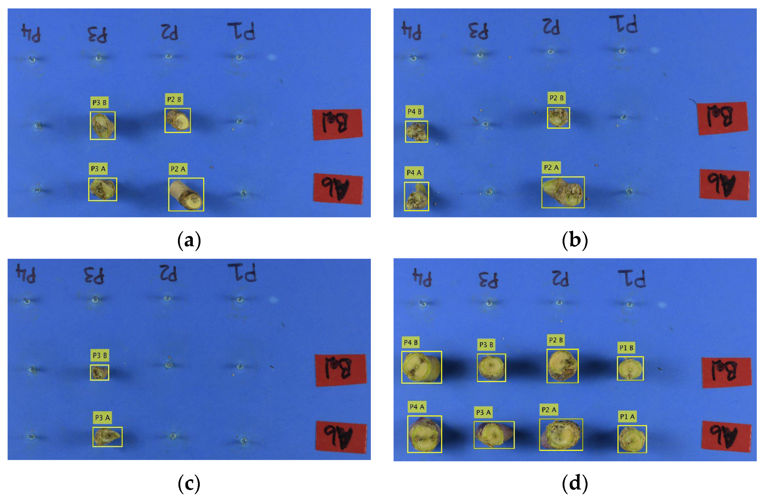
Digital images with the resolution of 6000 × 4000 pixels were captured using a Nikon d7200 camera, which is a DSLR camera featuring a 24.2-megapixel DX-format CMOS sensor, EXPEED 4-image processor, and 51-point autofocus system, offering high-quality images and advanced focusing capabilities. Each plant was cut transversely at the crown (the tissue where the stem meets the root) with secateurs to divide the plant into stem and root sections. A 2 cm section above the crown (labeled ‘Ab’) and a 2 cm section below the crown (labeled ‘Bel’) were produced by cutting transversely. Two images were captured for plants, with each image containing plant sections from a maximum of four plants placed at locations P1, P2, P3, or P4 (Figure 1). The first image captured the same cross-sectional surface of the ‘Above’ and ‘Below’ sections at the location of the crown. After the first image was captured, each ‘Above’ and ‘Below’ section was cut vertically, resulting in four longitudinal sections. The second image captured the longitudinal sections positioned in the same locations P1, P2, P3, or P4 as the first image. A barcode identifier was positioned in each image to link the plants. The blue background in the images was intentionally chosen to create a high contrast between the plants in the foreground and the background. Blue is not typically present in plant structures and hence provides high contrast, which is important for our algorithm to effectively distinguish and extract individual plants from the images. By using a blue background, we ensure that the plant extraction process is more accurate and efficient, as the distinct color difference minimizes errors in segmentation.
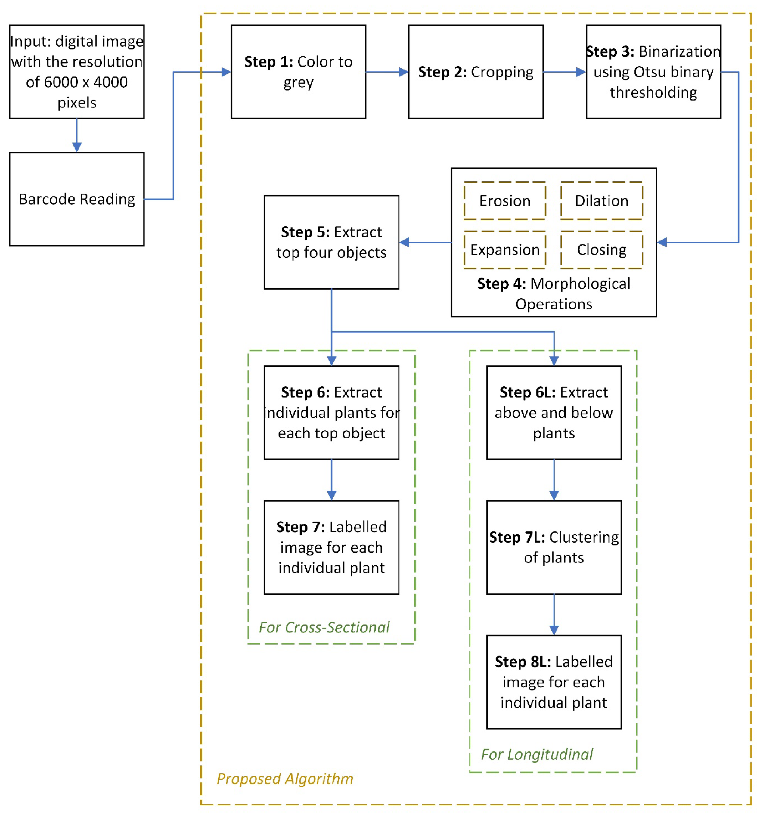
The goal was to develop an effective and efficient algorithm capable of extracting the cross-sections and longitudinal sections of each plant, as well as identify their position in terms of Ab or Bel and in position P1, P2, P3, or P4 to enable linkage to treatment and experimental information in addition to phenotype data captured during plant growth. Moreover, the algorithm was required to be sufficiently robust to cater for the variable conditions in each digital image, such as lighting, background, spacing between the plants, plant size, and position. The top-level block description of the image processing workflow is shown in Figure 2. The workflows for the extraction of cross-sections and longitudinal sections of each plant were similar except that an additional step was included to cluster plant parts for longitudinal sections. The barcode was read using a barcode scanner algorithm [34], with the subsequent workflow being undertaken in the following steps to extract the individual plants:
Step 1—Cropping: Let I be the original image with X number of rows, Y number of columns, and Z number of frames. There are three frames in I , red, green, and blue, represented as R ,   G , and B , respectively. Furthermore, let I ( x , y , z ) [ 0,255 ] be the value of an image pixel at x t h row, y t h column, and z t h frame. Once the barcode is read, the digital image was cropped horizontally to remove the part lacking useful information. The resulting image size was reduced by 30%, significantly reducing the computational burden and the possibility of false results. The cropped parts for Figure 1a–d are shown beneath the black line.
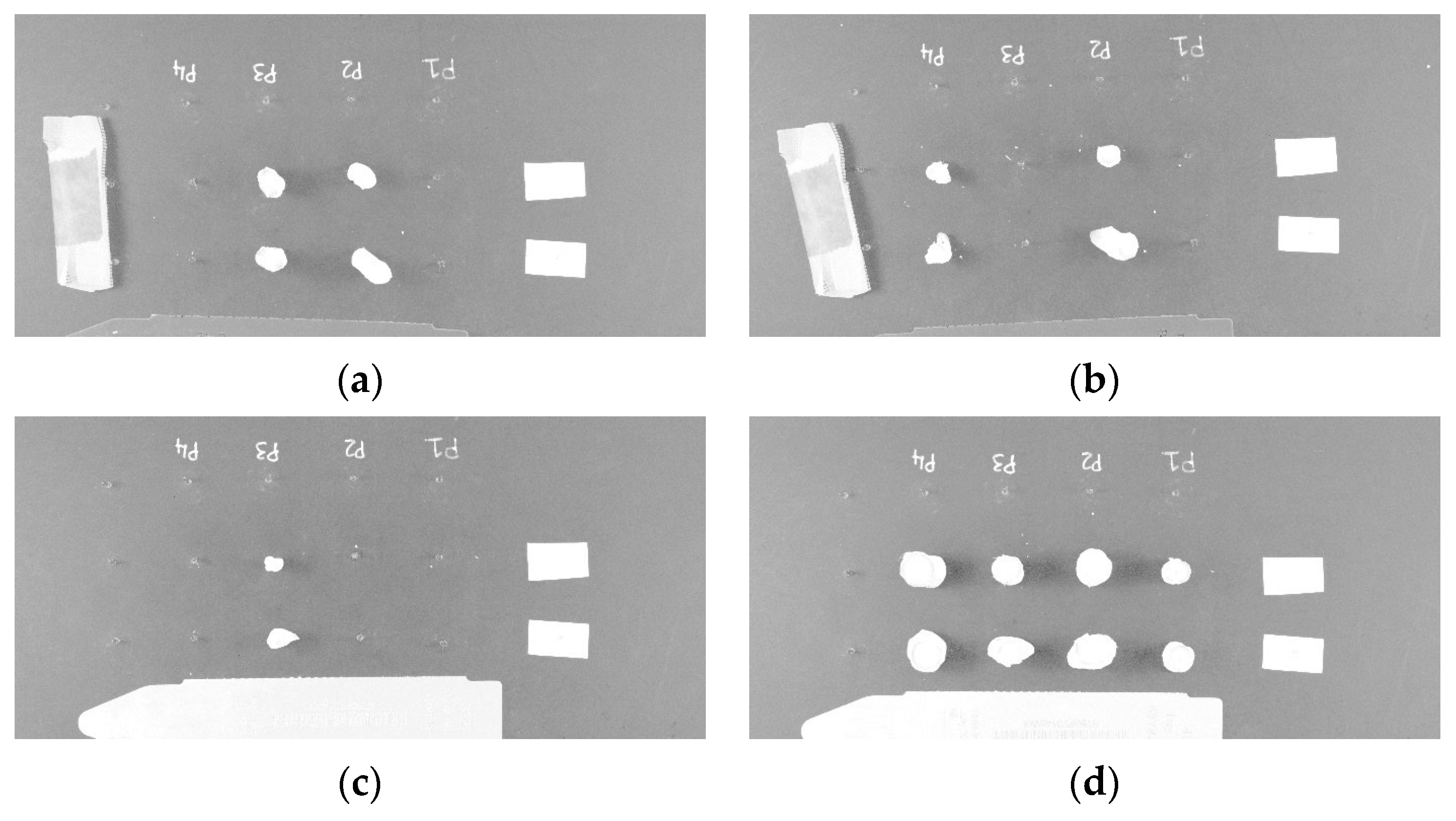
Step 2—Color to grey: The next step is the differentiation of the individual plant sections from the background. This was performed by applying a vegetation index, which identifies the green part in the digital image. There are numerous published vegetation indices, including the difference vegetation index [35], normalized difference vegetation index [36], modified simple ratio [37], transformed vegetation index [38], ratio vegetation index [39], and modified transformed vegetation index [40]. Each vegetation index was assessed for suitability to extract the plant sections from the digital images, with the ratio vegetation index [39] being most reliably able to separate the plant sections from the background and identify the P1, P2, P3, and P4 positions (Figure 3). The ratio vegetation index is applied on I to obtain the greenness, given as:
I g x , y = R I x , y , z G I x , y , z ,     x 1 ,   X ,   y 1 ,   Y ,   z 1 ,   Z ,  
where I g is the gray image representing the greenness of I ,   G is the green band, and R is the red band in I . The brighter pixels in Figure 3 represent the greenness and other objects, and the darker pixels represent the background. The values of these pixels are between [0, 255].
Step 3—Binarization: To categorize the pixels as either green (plant) or background, binarization was applied by setting a threshold. Pixels above the threshold are classified as green (plant), and the remainder is classified as background. The threshold value changes depending on the background conditions of the image. Manually setting a threshold for every digital image is inefficient. Instead, the Otsu binary thresholding method was applied [41] to automatically optimize the threshold value for each image, t h O t s u , to generate the binary image, I b :
I b x , y = 1         i f   I g x , y > t h O t s u ,   0         o t h e r w i s e ,         x 1 ,   X ,   y 1 ,   Y .  
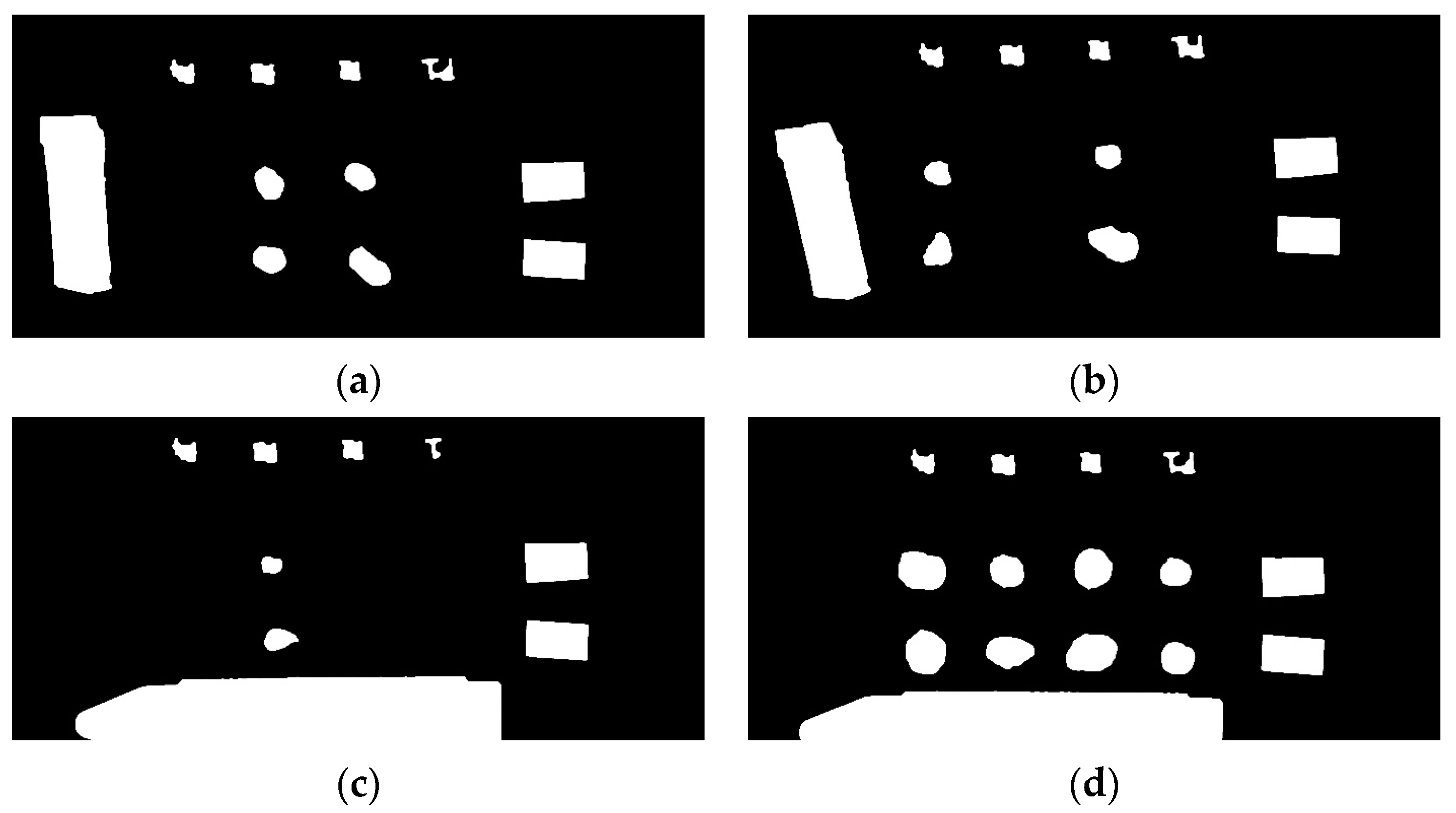
Figure 4a–d illustrates the binarization using Otsu thresholding applied to the images in Figure 3. The white pixels show the greenness, and the dark pixels show the background.
Step 4—Morphological operations: There are numerous small clusters of white pixels, which create a significant amount of noise (Figure 4). This noise was removed with the binopen function (in the MATLAB programming environment) in which image pixels with connected components that have fewer than m pixels are eliminated. The binopen function is defined as follows: each connected component in the binary image, I b , is labeled uniquely, I L = l a b e l ( I b ) . The number of pixels in each connected component k is calculated as C k = i , j ( I L = k ) . Finally, the pixels of components smaller than m are set to zero: I b = k ( C k m ) . ( I L = k ) . In this instance, the value of m is set to 1000. After the removal of noise, the rest of the connected image pixels are expanded by applying the image dilation function [39]:
I b s t = z | s t s z     I b ,  
where s t is a structuring element, s t s is the symmetric of s t , is a binary image dilation operation of s t on I b , z is a translation vector with the point ( z 1 , z 1 ) , is the translation of by the point s t s z s t s , is an intersection operator, and is an empty set. The image dilation function can also be written as [42]:
I b s t = z s t I b z ,    
where I b z is the translation of I b by the point z = ( z 1 , z 1 ) . To expand the image pixels, the structuring element used in this work is a disk of size 8 × 6. The resulting image contains the expanded binary objects. To further remove any smaller objects, the b i n o p e n function is applied again, with the value of m being set to 10,000. The binary objects, which are close enough to each other, are then joined together using a closing function, defined as [42]:
I b   s t = I b s t s t ,    
where is a closing function and is a binary erosion operation, defined as [42]:
I b s t = z | s t z I b c ,  
where ( . ) c is a compliment or logical NOT operator. The erosion, dilation, expansion, and closing functions are applied to images in Figure 4 with the results visible in Figure 5. The background noise is removed, and the binary objects are clearly visible.
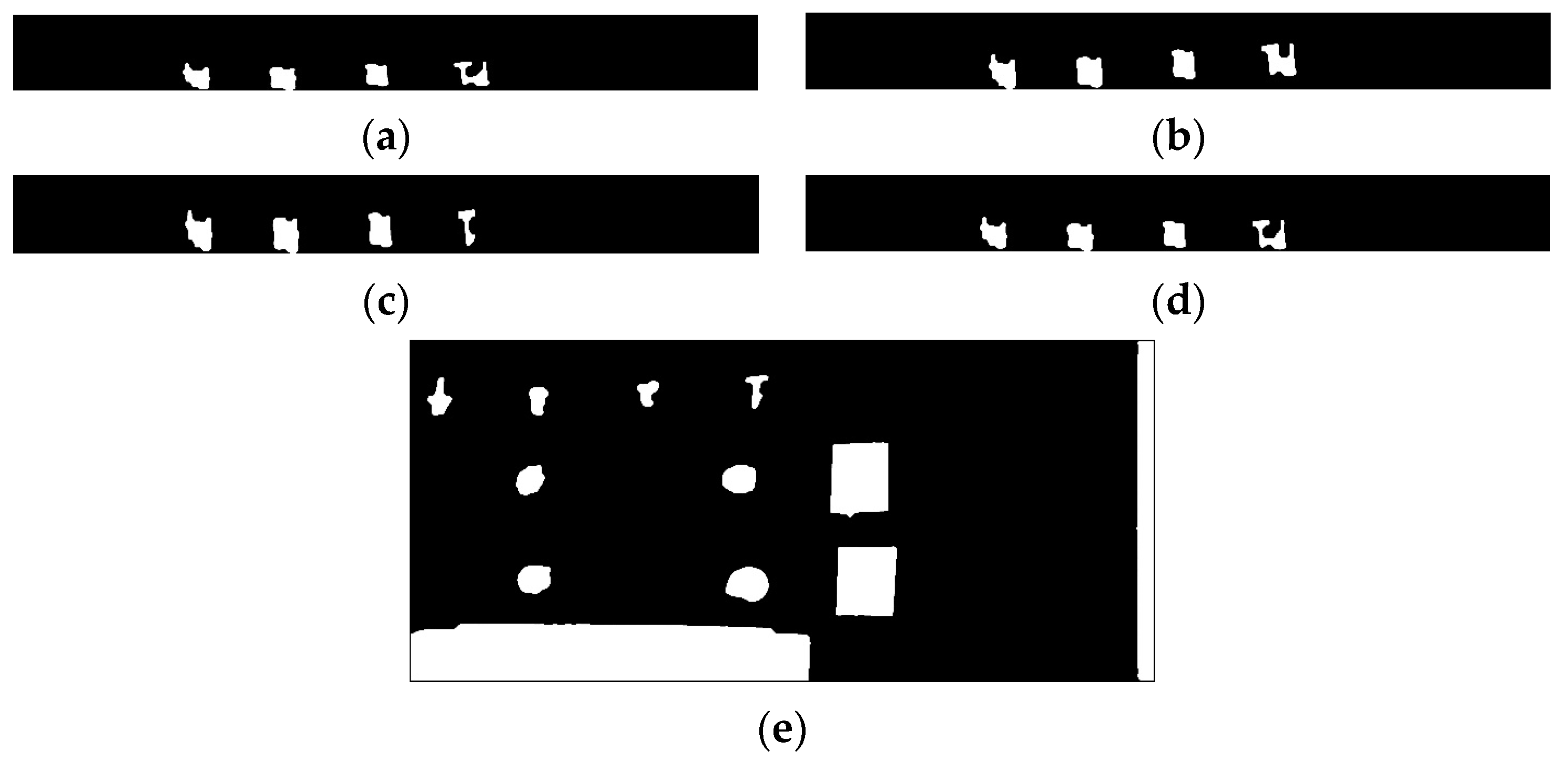
Step 5—Extracting the top four objects: The four binary objects corresponding to the labels of plants in positions P1, P2, P3, and P4 are detectable as individual objects and are present in every image, irrespective of whether there are any plant sections located beneath them. The locations and sizes of these four binary objects is facilitated by the fact that these objects are located at top of the digital image, allowing the locations to be extracted by sorting the objects in the digital image row-wise and then picking the first four row-wise sorted objects. These sorted objects correspond to the four positions: P1, P2, P3, and P4. In some images, there is a false object at the very top. To avoid this, the first five row-wise sorted objects are picked instead of the first four row-wise sorted objects. These five objects are sorted column-wise, and the first four column-wise-sorted objects extracted, which correspond to the four positions, are as illustrated in Algorithm 1 (Figure 6). Figure 6e shows an image with a false object at the top right.
Step 6—Extracting individual plants: Once the top four binary objects are obtained, the final task of extracting the individual plant sections beneath them (if there are any individual plants) is relatively simple (Figure 7). For every object in I t , the number of binary objects beneath that specific object is checked to confirm there are no more than two objects. If there are more than two objects, there could be false objects in addition to the individual plant sections. In the situation that more than two objects are detected, only the first two objects are extracted and declared as objects of interest. The top object is given location B and the second object is given the location A (Algorithm 2).
Algorithm 1.   The   process   of   extracting   the   four   binary   objects   corresponding   to   the   positions   P 1 ,   P 2 ,   P 3 ,   and   P 4   from   the   binary   image   I b .
Inputs:   Binary   image ,   I b .
Outputs:   Binary   image   containing   the   top   four   objects   only ,   I t .
1:
o b j s = b i n a r y _ o b j e c t s I b
2:
o b j s _ r o w = s o r t _ r o w _ w i s e o b j s
3:
I t = a s c e n d ( o b j _ r o w , 4 )
4:
I t _ o b j = b i n a r y _ o b j e c t s I t
5:
i f   l e n g t h I t _ o b j > 4
6:
    o b j _ c o l = s o r t _ c o l _ w i s e I t _ o b j
7:
    I t = a s c e n d ( o b j _ c o l , 4 )
Step 7—Plant labeling: Each extracted plant section is labeled with one of the four top positions P1, P2, P3, and P4, indicating Plants 1–4, and with one of two locations, indicating the section above or below the crown.
Algorithm 2. The process of extracting individual plants from I t .
Inputs: Binary image, I t .
Outputs: Individual plants, P l .
1:
o b j s = b i n a r y _ o b j e c t s I t
2:
f o r   i = 1   t o   l e n g t h o b j s  
3:
                  I t = c r o p p e d _ r o w I t o b j s i
4:
                o b j _ r = b i n a r y _ o b j e c t s I r
5:
                i f   l e n g t h o b j _ r > 2
6:
                                      f o r   j = 1   t o   2
7:
                                                        P l = e x t r a c t _ p l a n t I r

Extraction of Longitudinal Plant

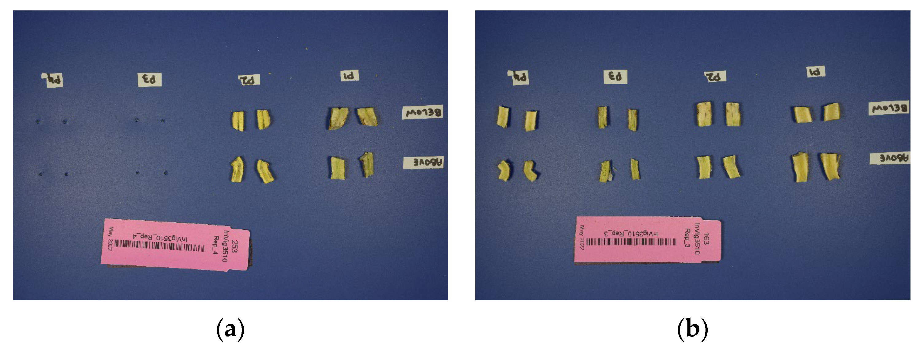
As described above, two types of images were captured for each set of plant samples: cross-sections (Figure 1) and longitudinal sections (Figure 8). Up to Step 5, the same process was applied for the extraction of the cross-section and longitudinal plant sections, i.e., the attainment of I b and I t (the top four objects corresponding to the four positions P1, P2, P3 and P4). Subsequent steps differed as follows:
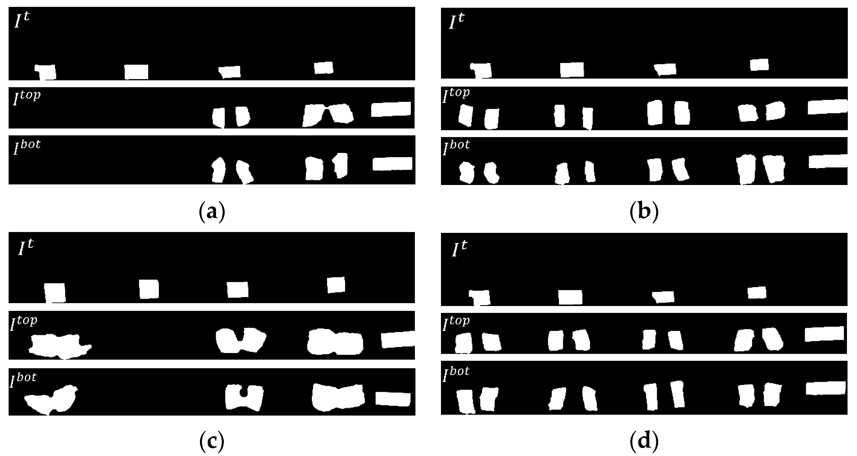
Step 6L—Extracting the above and below plants: From I b , the next step is to obtain the top image, which contains only the ‘Below’ sections, and the bottom image, which contains only the ‘Above’ sections (Figure 8). The number of binary objects and their bounding boxes are identified in I b . For each binary object in I b , the starting row position is compared with the starting row position of the immediate next binary object. If the difference in image pixels is more than m 3 , then the two binary objects are identified as objects, which belong to different parts of the image. The first object will be associated with the top image, I t o p , and the second object with the bottom image, I b o t . Furthermore, the remaining objects will be associated with I t o p , whose starting row position is less than the row position of the first object; otherwise, it will be associated with I b o t . Figure 9 shows the I t , I t o p , and I b o t images for Figure 8, respectively.
Step 7L—Clustering of plants: To associate each plant part in I t o p and I b o t with one of the four respective plant positions P1, P2, P3, and P4, the centroid (center point of the object in terms of row and column) of each object in I t is first computed, given as c e n i ,     i 1,2 , 3,4 . Then, the centroid is computed for each binary object in I t o p and I b o t , given as c e n _ t o p j ,     j 1,2 , ,   N t ,   c e n _ b o t j ,     j 1,2 , ,   N b , where N t and N b are the total number of binary objects in I t o p and I b o t , respectively. The difference between c e n _ t o p j ,     c e n _ b o t j , and c e n i is computed as follows:
d i f f _ t o p i ,   j = c e n i c e n t o p j ,           i 1,2 , 3,4 ,         j 1,2 , ,   N t .    
d i f f _ b o t i ,   j = c e n i c e n b o t j ,           i 1,2 , 3,4 ,         j 1,2 , ,   N b .  
The minimum values and their index positions from d i f f _ t o p i ,   j and d i f f _ b o t i ,   j are computed, where the index positions correspond to one of the four respective positions P1, P2, P3, and P4, given as:
m i n ,   i n d e x _ t o p j = m i n d i f f _ t o p : ,   j ,           j 1,2 , ,   N t .  
m i n ,   i n d e x _ b o t j = m i n d i f f _ b o t : ,   j ,           j 1,2 , ,   N b .  
Step 8L—Plant labeling: Finally, the binary objects with the same index positions are grouped together and labeled with either ‘Above’ or ‘Below’ and the plant identifier P1, P2, P3, or P4. Figure 10 shows the results of applying Steps 1–8 on Figure 8 to extract the longitudinal sections.

3. Evaluation Metrics

Several metrics were used to evaluate the performance of the work after applying the algorithm with optimized hyper-parameters to 722 cross-sectional and 313 longitudinal images (Table 1). Readers can implement the algorithm by applying the same optimized hyper-parameters presented in this study. These parameters [43] are:
Accuracy: accuracy, in the context of plant identification, refers to the number of plants correctly identified out of the total number of plants assessed, expressed as a percentage.
True positive rate (TPR): the percentage of correctly identified plants in the image. This is the same as the accuracy described above.
False positive rate (FPR): the percentage of falsely identified individual plants in each image.
True negative rate (TNR): the percentage of correctly detected non-plants in the image, such that TNR = 1 − FPR.
False negative rate (FNR): the percentage of incorrectly detected individual plant sections in the image.
Sensitivity: the proportion of actual positives (TPR) observed across the range of a specific parameter when all other parameters are kept constant at their optimized values.
Specificity: the proportion of actual negatives (TNR or 1 − FPR) observed across the range of a specific parameter when all other parameters are kept constant at their optimized values.
The receiver operating characteristic (ROC) curve: a graphical representation used in binary classification to assess the performance of a model. It plots the trade-off between the TPR (sensitivity) and FPR (one-specificity) across different threshold values, helping to visualize the model’s ability to discriminate between classes at various decision thresholds.

4. Results and Discussion

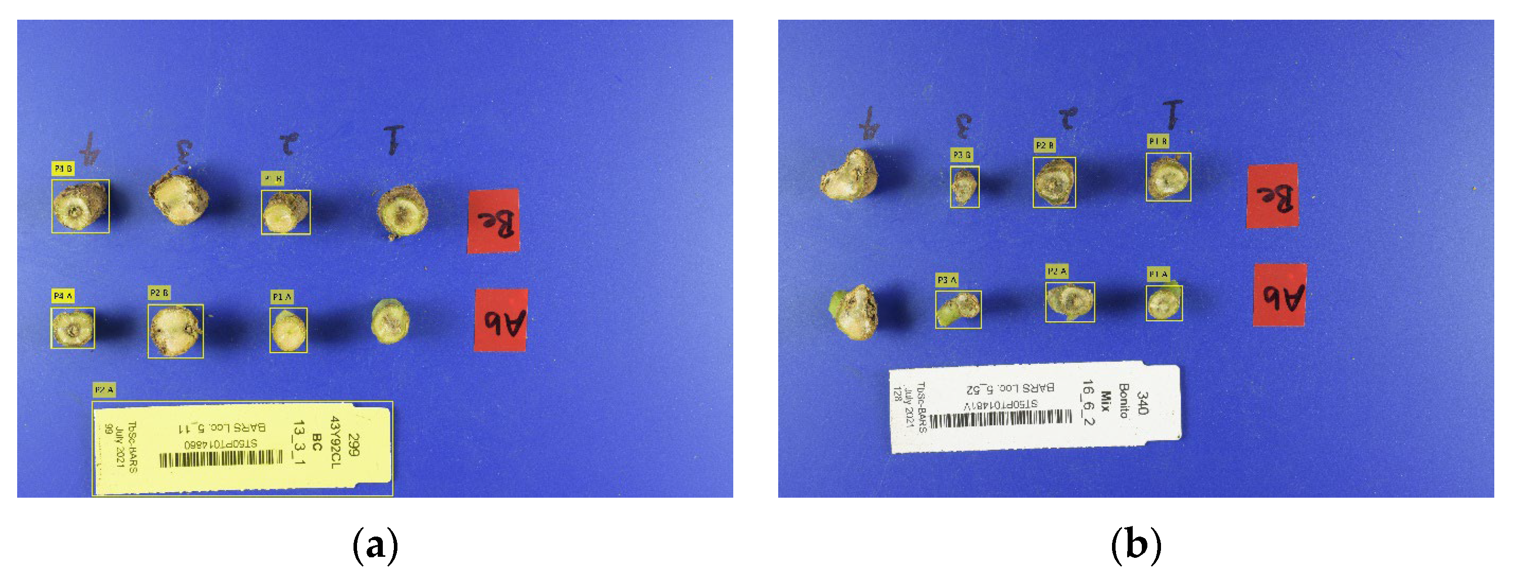
A variety of performance statistics were calculated to assess the performance of the algorithm. Overall, the percentage of correctly identified individual plant sections in each image (accuracy) for cross-sectional and longitudinal images was 98% and 86%, respectively. Accuracy is one measure to evaluate the performance of an algorithm but is insufficient for assessing the overall robustness as it can be misleading. For example, the same accuracy would be given for an image in which plant sections were correctly identified irrespective of whether they were identified in the correct positions (Figure 11).
The ROC is an enhanced performance indicator that incorporates the metrics of TPR, FPR, TNR, and FNR. The TPR is equivalent to accuracy and stands at 62.5% for the image depicted in Figure 11a and 75% for the image in Figure 11b. In the dataset in this study, the mean TPR is 98% for cross-sectional images and 86% for longitudinal images. FPR signifies falsely identified individual plants. In Figure 11a, one position is falsely identified, resulting in an FPR of 12.5% (1/8) for that image. Conversely, in Figure 11b, there are no falsely identified positions, such that FPR is 0%. The mean FPR is consistent at 3% for both cross-sectional and longitudinal images. As TNR is the complement of FPR (1-FPR), the mean TNR for both cross-sectional and longitudinal images is 97%. Specifically, for Figure 11a,b, the TNR is 87.5% and 0%, respectively. Lastly, FNR is the complement of TPR (1-TPR) such that the mean FNRs for cross-sectional and longitudinal images are 2% and 14%, respectively. In Figure 11a, three plant sections go unidentified despite their actual presence in the correct location, resulting in an FNR of 37.5% (3/8). Similarly, in Figure 11b, two plant sections fail to be identified despite their actual presence, leading to an FNR of 25% (2/8).
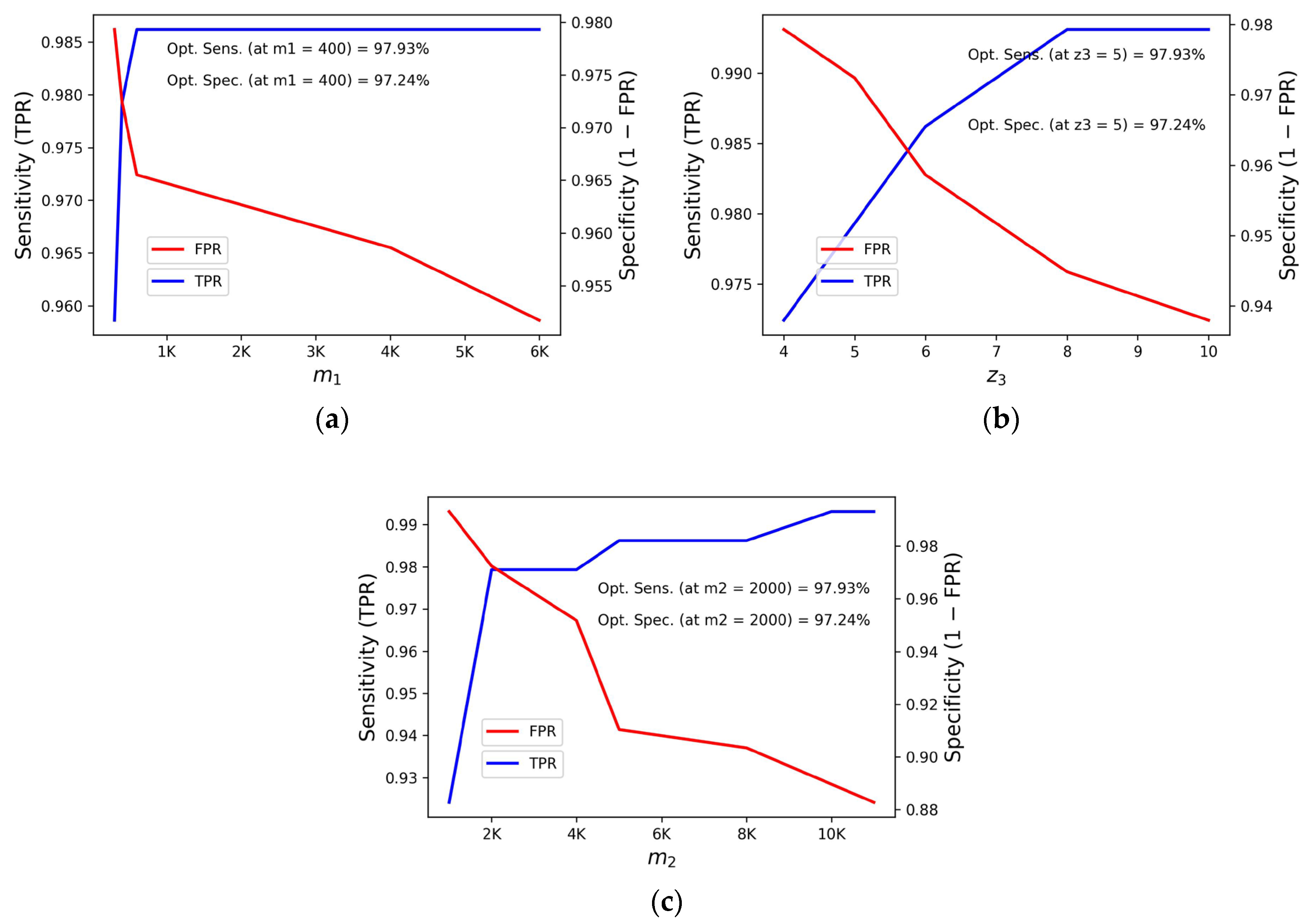
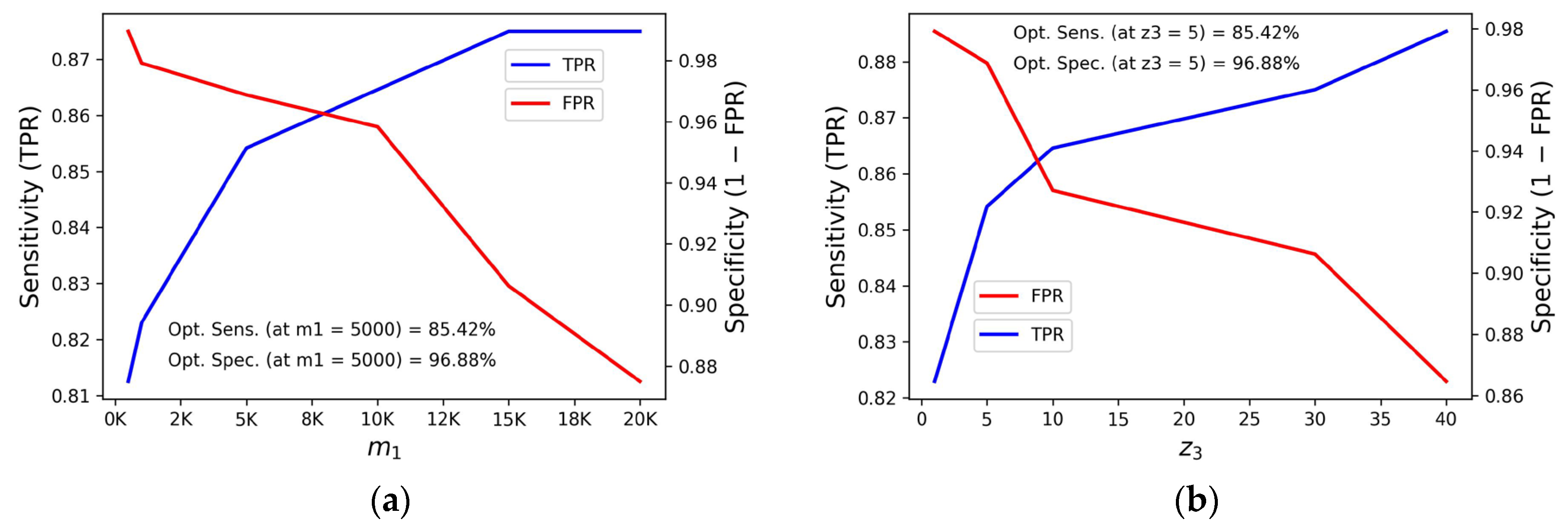
Sensitivity and specificity graphs were generated for both the cross-sectional and longitudinal datasets across different parameter values to identify optimized values. For cross-sectional images, the maximum sensitivity values were: m 1 = 98.62, z 3 = 99.31, and m 2 = 99.31, and the specific parameter values at which the sensitivity was optimized were as follows: m 1 reaches 97.93% at m 1 = 400, z 3 achieves 97.93% sensitivity at z 3 = 5, and m 2 reaches its peak sensitivity of 97.93% at m 2 = 2000 (Figure 12). Similarly, the maximum specificity values were: m 1 and z 3 = 97.93 and m 2 = 99.31; the optimized specificity values were as follows: m 1 reaches 97.24% at m1 = 400, z 3 attains 97.24% specificity at z 3 = 5, and m 2 exhibits 97.24% specificity at m 2 = 2000. For the longitudinal images, the maximum sensitivity values were: m 1 = 87.50 and z 3 = 88.54, and the optimized sensitivity values for both were 96.88% at m 1 = 5000 and z 3 = 5 (Figure 13).
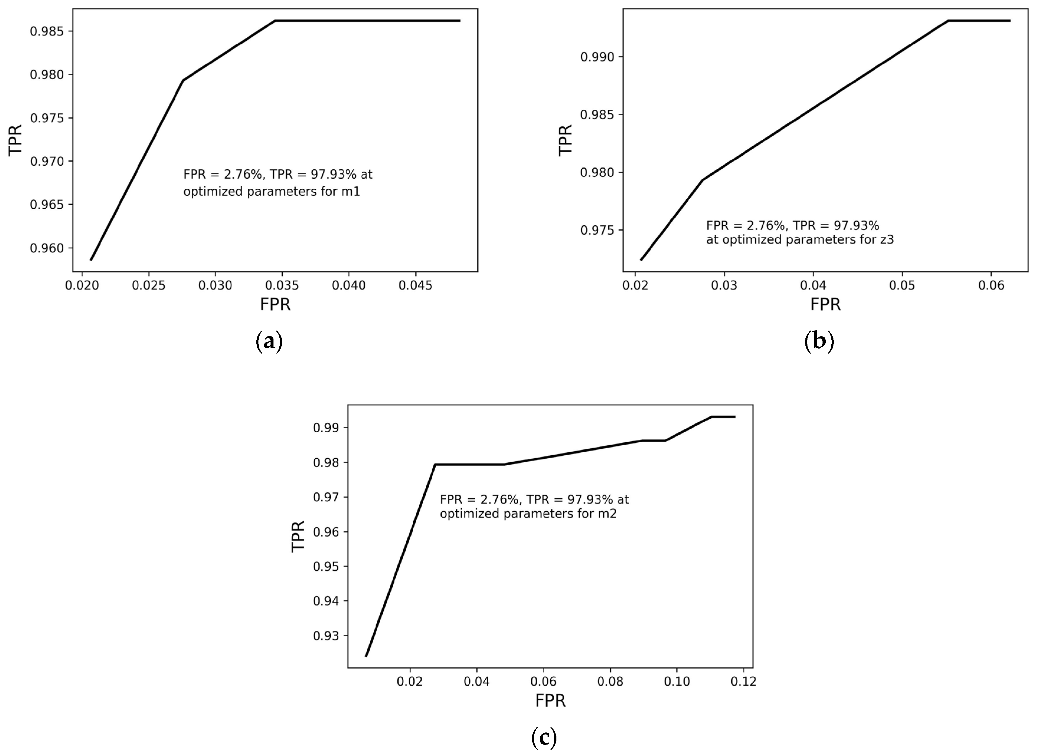
Finally, the ROC plotted between TPR and FPR can be used to assess the overall performance and robustness of the algorithm and to select the optimized values for each parameter. For both the cross-sectional (Figure 14) and longitudinal images (Figure 15), there is a positive relationship between TPR and FPR for each of the parameters. Therefore, identifying an appropriate value for a parameter should be based on both performance criteria of TPR and FPR. This workflow is repeatable and adaptable to a wide range of images captured from the top view (assuming modified and appropriate hyper-parameter values), although it is strongly recommended to perform an analysis and tuning of the parameters listed in Table 1 before deployment to a new dataset.
The image-based algorithm allows for the extraction and spatial labeling of up to eight individual plants within RGB images captured under controlled conditions. This is the first step towards the development of an accurate disease quantification tool for blackleg crown canker in canola by using approaches such as unsupervised pixel-level thresholding or supervised machine learning on extracted images. The high true positive rates (TPR) and low false positive rates (FPR) computed for a range of different values of hyper-parameters demonstrate the robustness of the proposed algorithm for the extraction of individual plants from images that differ in lighting conditions, positioning of objects within the image, and spacing between the objects. While this algorithm was specifically developed to address an existing technological gap for more high-throughput approaches to phenotype blackleg crown canker disease, there is an increasing requirement for large phenotypic datasets to support the implementation of advanced genetic approaches for plant breeding [14,15]. As such, the integration of image-based and other digital methods for disease quantification will be required to achieve sustainable, profitable, and equitable food production. The current algorithm has been tested in a controlled environment with future work underway to translate it to images captured under field conditions.

5. Conclusions

The algorithm was able to extract individual plant sections from RGB images and allocate them to the correct experimental replicate (P1, P2, P3, and P4) and position (above or below). The algorithm consists of various image processing operations, including binarization, cropping, erosion, and dilation. The proposed work is effective and efficient, with an accuracy rate of 98% and 86% when applied to 722 cross-sectional and 313 longitudinal images, respectively. The true positive rates (TPRs) and false positive rates (FPRs) computed for a range of different values of hyper-parameters demonstrate the robustness of the proposed algorithm. The algorithm is sufficiently robust to extract the objects under different lighting conditions, positioning of objects within the image, and spacing between the objects. Therefore, it has application for a wide range of plant images taken from a top view (assuming modified and appropriate hyper-parameter values), although it is strongly recommended to perform analysis and tuning of the parameters listed in Table 1 before deployment to a new dataset. This algorithm is the foundation for developing a pipeline for the automated assessment of blackleg crown canker severity using RGB images. It aims to support the global research community by facilitating breeding for canola cultivars with increased blackleg resistance, the development of control strategies, and the advancement of knowledge on plant–pathogen interactions.

Author Contributions

Conceptualization, S.R., L.B. and S.S.; methodology, S.R. and S.S.; software, S.S.; validation, S.R., L.B., W.S., R.M. and S.S.; data curation, L.B., W.S., R.M. and S.S.; writing—original draft preparation, S.R.; writing—review and editing, L.B., W.S., R.M. and S.S.; supervision, S.S.; project administration, L.B. and S.S. All authors have read and agreed to the published version of the manuscript.

Funding

This research received funding from the Australian Grains Research and Development Corporation (GRDC) (CSP1904-007RTX and CSP2307-006RTX).

Data Availability Statement

The raw data supporting the conclusions of this article will be made available by the authors on request.

Acknowledgments

The authors acknowledge the financial support of CSIRO and the GRDC to conduct this research.

Conflicts of Interest

The authors declare no conflicts of interest.

References

  1. Wani, N.R.; Rather, R.A.; Farooq, A.; Padder, S.A.; Baba, T.R.; Sharma, S.; Mubarak, N.M.; Khan, A.H.; Singh, P.; Ara, S. New insights in food security and environmental sustainability through waste food management. Environ. Sci. Pollut. Res. 2024, 31, 17835–17857. [Google Scholar] [CrossRef] [PubMed]
  2. Qamer, F.M.; Abbas, S.; Ahmad, B.; Hussain, A.; Salman, A.; Muhammad, S.; Nawaz, M.; Shrestha, S.; Iqbal, B.; Thapa, S. A framework for multi-sensor satellite data to evaluate crop production losses: The case study of 2022 Pakistan floods. Sci. Rep. 2023, 13, 4240. [Google Scholar] [CrossRef] [PubMed]
  3. G-Domínguez, E.; Caffi, T.; Rossi, V.; Salotti, I.; Fedele, G. Plant Disease Models and Forecasting: Changes in Principles and Applications over the Last 50 Years. Phytopathology 2023, 113, 678–693. [Google Scholar] [CrossRef] [PubMed]
  4. Siddiqui, J.A.; Fan, R.; Naz, H.; Bamisile, B.S.; Hafeez, M.; Ghani, M.I.; Wei, Y.; Xu, Y.; Chen, X. Insights into insecticide-resistance mechanisms in invasive species: Challenges and control strategies. Front. Physiol. 2023, 13, 1112278. [Google Scholar] [CrossRef]
  5. Shi, T.; Liu, Y.; Zheng, X.; Hu, K.; Huang, H.; Liu, H.; Huang, H. Recent advances in plant disease severity assessment using convolutional neural networks. Sci. Rep. 2023, 13, 2336. [Google Scholar] [CrossRef]
  6. Xie, Y.; Plett, D.; Liu, H. The Promise of Hyperspectral Imaging for the Early Detection of Crown Rot in Wheat. AgriEngineering 2021, 3, 924–941. [Google Scholar] [CrossRef]
  7. Cianchetta, A.N.; Davis, R.M. Fusarium wilt of cotton: Management strategies. Crop Prot. 2015, 73, 40–44. [Google Scholar] [CrossRef]
  8. D-Daigle, P.; Kirkby, K.; Chowdhury, P.R.; Labbate, M.; Chapman, T.A. The Verticillium wilt problem in Australian cotton. Australas. Plant Pathol. 2021, 50, 129–135. [Google Scholar] [CrossRef]
  9. Wouw, A.P.V.D.; Scanlan, J.L.; Al-Mamun, H.A.; Balesdent, M.H.; Bousset, L.; Burketová, L.; del Rio Mendoza, L.; Fernando, W.D.; Franke, C.; Howlett, B.J.; et al. A new set of international Leptosphaeria maculans isolates as a resource for elucidation of the basis and evolution of blackleg disease on Brassica napus. Plant Pathol. 2024, 73, 170–185. [Google Scholar]
  10. Sprague, S.; de Wouw, A.V.; Marcroft, S.J.; Geffersa, A.G.; Idnurm, A.; Barrett, L. Host genetic resistance in Brassica napus: A valuable tool for the integrated management of the fungal pathogen Leptosphaeria maculans. Am. Phytopathol. Soc. 2024. ahead of print. [Google Scholar] [CrossRef]
  11. Sprague, S.J.; Marcroft, S.J.; Hayden, H.L.; Howlett, B.J. Major Gene Resistance to Blackleg in Brassica napus Overcome Within Three Years of Commercial Production in Southeastern Australia. Am. Phytopathol. Soc. 2006, 90, 190–198. [Google Scholar] [CrossRef] [PubMed]
  12. Bondad, J.; Harrison, M.T.; Whish, J.; Sprague, S.; Barry, K. Integrated crop-disease models: New frontiers in systems thinking. Farm. Syst. 2023, 1, 100004. [Google Scholar] [CrossRef]
  13. Schnippenkoetter, W.; Hoque, M.; Maher, R.; Van de Wouw, A.; Hands, P.; Rolland, V.; Barrett, L.; Sprague, S. Comparison of non-subjective relative fungal biomass measurements to quantify the Leptosphaeria maculansBrassica napus interaction. Plant Methods 2021, 17, 112. [Google Scholar] [CrossRef] [PubMed]
  14. Pathania, A.; Rialch, N.; Sharma, P.N. Marker-Assisted Selection in Disease Resistance Breeding: A Boon to Enhance Agriculture Production. Curr. Dev. Biotechnol. Bioeng. 2017, 187–213. [Google Scholar] [CrossRef]
  15. Alemu, A.; Åstrand, J.; Montesinos-Lopez, O.A.; y Sanchez, J.I.; Fernandez-Gonzalez, J.; Tadesse, W.; Vetukuri, R.R.; Carlsson, A.S.; Ceplitis, A.; Crossa, J.; et al. Genomic selection in plant breeding: Key factors shaping two decades of progress. Mol. Plant 2024, 17, 552–578. [Google Scholar] [CrossRef] [PubMed]
  16. Nguyen, T.K.; Dang, M.; Doan, T.T.M.; Lim, J.H. Utilizing Deep Neural Networks for Chrysanthemum Leaf and Flower Feature Recognition. AgriEngineering 2024, 6, 1133–1149. [Google Scholar] [CrossRef]
  17. Sanaeifar, A.; Yang, C.; de la Guardia, M.; Zhang, W.; Li, X.; He, Y. Proximal hyperspectral sensing of abiotic stresses in plants. Sci. Total Environ. 2023, 861, 160652. [Google Scholar] [CrossRef]
  18. Sarić, R.; Nguyen, V.D.; Burge, T.; Berkowitz, O.; Trtílek, M.; Whelan, J.; Lewsey, M.G.; Čustović, E. Applications of hyperspectral imaging in plant phenotyping. Trends Plant Sci. 2022, 27, 301–315. [Google Scholar] [CrossRef]
  19. Olumurewa, K.O.; Eleruja, M.A. Photoelectrical and thermal sensing measurement of spin coated ZnO and ZnO-RGO thin film. Phys. B Condens. Matter 2023, 650, 414588. [Google Scholar] [CrossRef]
  20. Xiong, Y.; Shepherd, S.; Tibbs, J.; Bacon, A.; Liu, W.; Akin, L.D.; Ayupova, T.; Bhaskar, S.; Cunningham, B.T. Photonic Crystal Enhanced Fluorescence: A Review on Design Strategies and Applications. Micromachines 2023, 14, 668. [Google Scholar] [CrossRef]
  21. Li, Y.; Yang, X.; Liang, X.; Zhang, K.; Liang, X. Au Experiment and Application of NATM Tunnel Deformation Monitoring Based on 3D Laser Scanning. Struct. Control Health Monit. 2023, 1, 3341788. [Google Scholar]
  22. Taparhudee, W.; Jongjaraunsuk, R.; Nimitkul, S.; Suwannasing, P.; Mathurossuwan, W. Optimizing Convolutional Neural Networks, XGBoost, and Hybrid CNN-XGBoost for Precise Red Tilapia (Oreochromis niloticus Linn.) Weight Estimation in River Cage Culture with Aerial Imagery. AgriEngineering 2024, 6, 1235–1251. [Google Scholar] [CrossRef]
  23. Fu, J.; Liu, J.; Zhao, R.; Chen, Z.; Qiao, Y.; Li, D. Maize Disease Detection Based on Spectral Recovery from RGB Images. Front. Plant Sci. 2022, 13, 1056842. [Google Scholar] [CrossRef] [PubMed]
  24. Meline, V.; Caldwell, D.L.; Kim, B.-S.; Khangura, R.S.; Baireddy, S.; Yang, C.; Sparks, E.E.; Dilkes, B.; Delp, E.J.; Iyer-Pascuzzi, A.S. Image-Based Assessment of Plant Disease Progression Identifies New Genetic Loci for Resistance to Ralstonia solanacearum in Tomato. Plant J. 2023, 113, 887–903. [Google Scholar] [CrossRef]
  25. Xie, Y.; Plett, D.; Liu, H. Detecting Crown Rot Disease in Wheat in Controlled Environment Conditions Using Digital Color Imaging and Machine Learning. AgriEngineering 2022, 4, 141–155. [Google Scholar] [CrossRef]
  26. McDonald, S.C.; Buck, J.; Li, Z. Automated, Image-Based Disease Measurement for Phenotyping Resistance to Soybean Frogeye Leaf Spot. Plant Methods 2022, 18, 103. [Google Scholar] [CrossRef]
  27. Mutka, A.M.; Bart, R.S. Image-Based Phenotyping of Plant Disease Symptoms. Front. Plant Sci. 2015, 5, 734. [Google Scholar] [CrossRef]
  28. Padmavathi, K.; Thangadurai, K. Implementation of RGB and Grayscale Images in Plant Leaves Disease Detection—Comparative Study. Indian J. Sci. Technol. 2016, 9, 1–6. [Google Scholar] [CrossRef]
  29. Shin, J.; Chang, Y.K.; Heung, B.; Nguyen-Quang, T.; Price, G.W.; Al-Mallahi, A. A Deep Learning Approach for RGB Image-Based Powdery Mildew Disease Detection on Strawberry Leaves. Comput. Electron. Agric. 2021, 183, 106042. [Google Scholar] [CrossRef]
  30. Li, X.; Hou, B.; Zhang, R.; Liu, Y. A Review of RGB Image-Based Internet of Things in Smart Agriculture. IEEE Sens. J. 2023, 23, 24107–24122. [Google Scholar] [CrossRef]
  31. Karisto, P.; Hund, A.; Yu, K.; Anderegg, J.; Walter, A.; Mascher, F.; McDonald, B.A.; Mikaberidze, A. Ranking Quantitative Resistance to Septoria Tritici Blotch in Elite Wheat Cultivars Using Automated Image Analysis. Dis. Control Pest Manag. 2018, 108, 568–581. [Google Scholar] [CrossRef] [PubMed]
  32. Jasim, M.A.; AL-Tuwaijari, J.M. Plant Leaf Diseases Detection and Classification Using Image Processing and Deep Learning Techniques. In Proceedings of the 2020 International Conference on Computer Science and Software Engineering (CSASE), Duhok, Iraq, 16–18 April 2020; IEEE: New York, NY, USA, 2020. [Google Scholar]
  33. Shoaib, M.; Shah, B.; Ei-Sappagh, S.; Ali, A.; Ullah, A.; Alenezi, F.; Gechev, T.; Hussain, T.; Ali, F. An Advanced Deep Learning Models-Based Plant Disease Detection: A Review of Recent Research. Front. Plant Sci. 2023, 14, 1158933. [Google Scholar]
  34. Mazakova, B.; Otarbaev, A. The Algorithm of Barcode Scanner. Science 2011, 12, 100. [Google Scholar]
  35. Jiang, Z. Analysis of NDVI and Scaled Difference Vegetation Index Retrievals of Vegetation Fraction. Remote Sens. Environ. 2006, 101, 366–378. [Google Scholar] [CrossRef]
  36. Pettorelli, N. The Normalized Difference Vegetation Index; Oxford University Press: Oxford, UK, 2013. [Google Scholar]
  37. Chen, J.M. Evaluation of Vegetation Indices and a Modified Simple Ratio for Boreal Applications. Can. J. Remote Sens. 1996, 22, 229–242. [Google Scholar] [CrossRef]
  38. Nellis, M.D.; Briggs, J.M. Transformed Vegetation Index for Measuring Spatial Variation in Drought Impacted Biomass on Konza Prairie, Kansas. Trans. Kans. Acad. Sci. 1992, 95, 93–99. [Google Scholar] [CrossRef]
  39. Major, D.J.; Baret, F.; Guyot, G. A Ratio Vegetation Index Adjusted for Soil Brightness. Int. J. Remote Sens. 1990, 11, 727–740. [Google Scholar] [CrossRef]
  40. Skianis, G.; Vaiopoulos, D.; Nikolakopoulos, K. A Comparative Study of the Performance of the NDVI, the TVI and the SAVI Vegetation Indices over Burnt Areas, Using Probability Theory and Spatial Analysis Techniques. In Towards An Operational Use of Remote Sensing in Forest Fire Management; European Commission: Brussels, Belgium, 2007; p. 149. [Google Scholar]
  41. Yousefi, J. Image Binarization Using Otsu Thresholding Algorithm; University of Guelph: Ontario, CA, USA, 2011. [Google Scholar]
  42. Gonzalez, R.C. Digital Image Processing; Pearson Education India: Hoboken, NJ, USA, 2009. [Google Scholar]
  43. Hanley, J.A. Receiver Operating Characteristic (ROC) Methodology: The State of the Art. Crit. Rev. Diagn. Imaging 1989, 29, 307–335. [Google Scholar]
Figure 1. (ad) Examples of digital images of canola plants with blackleg disease cut transversely to reveal the cross-section. The arrangement of each image consists of a maximum of four plants of two sections each (total: eight plant sections). Images have variable lighting conditions, backgrounds, spacing between sections, section sizes and position, as well as barcode tag color. The cropped parts are beneath the black line. (e) Zoomed in image of 1 (d).
Agriengineering 06 00199 g001
Figure 2. A top-level block description of the developed work.
Agriengineering 06 00199 g002
Figure 3. (ad) The same images shown in Figure 1a–d, respectively, with the ratio vegetation index applied to identify the plant sections and position P1, P2, P3, and P4. The index was applied to the cropped images to reduce the computation burden and likelihood of false results.
Agriengineering 06 00199 g003
Figure 4. (ad) The same images shown in Figure 3a–d, respectively, with the binarization applied using Otsu binary thresholding. There are only two grey scales: white, which represents the greenness; and black, which represents the background.
Agriengineering 06 00199 g004
Figure 5. (ad) The images shown in Figure 4a–d, respectively, with the erosion, dilation, expansion, and closing applied. All noise has been removed, and the connected image pixels are clearly visible for the individual plant sections and their positions.
Agriengineering 06 00199 g005
Figure 6. (ad) The same images in Figure 5a–d, respectively, with the first four binary objects corresponding to the labels of the positions P1, P2, P3, and P4. (e) False object shown at the right side.
Agriengineering 06 00199 g006
Figure 7. (ad) The individual plant sections are extracted and labeled with one of the four top positions (P1, P2, P3, or P4) and with one of two locations (A or B).
Agriengineering 06 00199 g007
Figure 8. (ad) The subset of digital images taken from the top view. Each digital image consists of maximum of eight plants with variable conditions. Furthermore, each plant has two longitudinal parts.
Agriengineering 06 00199 g008aAgriengineering 06 00199 g008b
Figure 9. (ad) The same images as in Figure 8, respectively, with the extraction of I t , I t o p , and I b o t . The I t o p and I b o t images show only the top and bottom plants, respectively.
Agriengineering 06 00199 g009
Figure 10. (ad) The same images as in Figure 8 with the individual longitudinal sections for each plant extracted and labeled with the plant position (P1, P2, P3, or P4) and location (A or B).
Agriengineering 06 00199 g010
Figure 11. Example images of (a) the false positive and negative detection of individual plants (the barcode is detected as a plant, while plants in 1A, 1B, and 3B are not detected), and (b) the false negative detection of individual plants (plants at 4A and 4B are not detected).
Agriengineering 06 00199 g011
Figure 12. Sensitivity and specificity graphs for the true positive rate for cross-sectional images plotted against a range of values for parameters m 1 (a), z 3   (b), and m 2   (c), respectively. Opt. Sens. = optimized sensitivity and Opt. Spec. = optimized specificity.
Agriengineering 06 00199 g012
Figure 13. (a,b) Sensitivity and specificity graphs for longitudinal images plotted against the ranges of m 1 and z 3 , respectively.
Agriengineering 06 00199 g013
Figure 14. Receiver operating characteristic (ROC) graphs for cross-sectional images plotted against the ranges of (a) m 1 , (b) z 3 , and (c) m 2 .
Agriengineering 06 00199 g014
Figure 15. Receiver operating characteristic (ROC) graphs for longitudinal images plotted against the ranges of (a) m 1 and (b) z 3 .
Agriengineering 06 00199 g015
Table 1. List of hyper-parameters and the optimized value used in Step 4.
SymbolDescriptionCross-SectionLongitudinal
m 1 Number of pixels for noise removal—Stage 14005000
m 2 Number of pixels for noise removal—Stage 22000Any
z 1 x-coordinate of translation vector to dilate the binary image44
z 2 y-coordinate of translation vector to dilate the binary image66
z 3 Radius of translation vector to dilate the binary image55
Disclaimer/Publisher’s Note: The statements, opinions and data contained in all publications are solely those of the individual author(s) and contributor(s) and not of MDPI and/or the editor(s). MDPI and/or the editor(s) disclaim responsibility for any injury to people or property resulting from any ideas, methods, instructions or products referred to in the content.