AI-Powered Evaluation of On-Demand Public Transport: A Hybrid Simulation Approach

Highlights

What are the main findings?

• A unified simulation framework combining agent-based modelling, BiLSTM demand forecasting, and behavioural survey calibration was demonstrated for evaluating on-demand public transport.
• Hybrid on-demand services achieved substantial performance gains, including shorter trips, reduced waiting times, higher vehicle occupancy, and significantly lower emissions.

What are the implications of the main findings?

• Integrating on-demand services with existing fixed routes can improve service quality, sustainability, and operational efficiency in urban public transport networks.
• The framework provides a transferable decision-support approach for testing fleet strategies, optimising depot siting, and guiding data-driven policy evaluation.

Abstract

On-demand public transport systems are increasingly adopted to improve service flexibility, reduce operating costs, and meet emerging mobility needs. Evaluating their performance under realistic demand and operational conditions, however, remains a complex challenge. This study presents a hybrid simulation framework that integrates deep learning-based demand forecasting, behavioural survey data, and agent-based simulation to assess system performance. A BiLSTM neural network trained on real-world smartcard data forecasts short-term passenger demand, which is embedded into an agent-based model simulating vehicle dispatch, routing, and passenger interactions. The framework is applied to a case study in Melbourne, Australia, comparing a baseline fixed-route service with two on-demand scenarios. Results show that the most flexible scenario reduces the average passenger trip time by 32%, decreases the average wait time by 34%, increases vehicle occupancy from 12.1 to 18.6 passengers per vehicle, lowers emissions per passenger trip by 72%, and cuts the service cost per trip from AUD 6.82 to AUD 4.73. These findings demonstrate the potential of hybrid on-demand services to improve operational efficiency, passenger experience, and environmental outcomes. The study presents a novel, integrated methodology for scenario-based evaluation of on-demand public transportation using real-world transportation data.

1. Introduction

The rapid evolution of digital platforms, mobile applications, and data-driven operations has created new opportunities for alternative mobility services that can complement traditional public transport. A growing motivation for such innovations stems from the poor performance of many fixed-schedule services during off-peak periods, alongside increasing expectations among digitally connected travellers for reliability, flexibility, and convenience [1,2]. Empirical evidence consistently shows that off-peak passenger demand on conventional bus routes can decline by 40–70% compared to peak periods, while operating costs remain largely fixed, resulting in low vehicle occupancy and high cost per passenger trip [3,4,5]. As cities pursue sustainable urban mobility, demand-responsive transport (DRT) systems offer an emerging pathway that balances service quality and operational efficiency, particularly in lower-density contexts or at non-peak times.

For decades, urban transport policy has disproportionately favoured private vehicle use, contributing to congestion, emissions, and unsustainable travel behaviour [6]. Private cars have long symbolised independence and flexibility, often receiving greater political and financial support than public transport modes. In contrast, buses (despite their potential for low-cost, scalable service delivery) have often suffered from inadequate investment and limited service quality, reducing their appeal to potential users [7,8,9,10]. This imbalance is especially evident outside peak commuting hours, where fixed-route services frequently operate with occupancy rates below 20–30%, undermining both economic viability and perceived service quality [5,11]. However, the proliferation of smart personal devices and mobile internet has enabled new forms of shared, app-based mobility services that can bridge the gap between private convenience and public efficiency [12,13,14,15,16].

On-demand public transport, also referred to as flexible transport, mobility-on-demand, or microtransit, is now seen as a promising solution that can serve areas and time periods not well covered by conventional services. These systems typically use algorithmically routed vehicles, often vans or minibuses, operating on flexible routes and schedules in response to real-time passenger requests. They are particularly well-suited to addressing first/last kilometre connectivity, off-peak service coverage, and mobility needs for groups such as older adults and people with disabilities [17,18,19,20,21]. By dynamically matching supply to demand, on-demand systems have been shown to reduce per-passenger operating costs by 20–50% in low-demand periods, while improving temporal availability and service responsiveness relative to fixed-route operations [9,11]. Operating models vary in sophistication, from pre-booked services with semi-fixed routes to fully dynamic systems integrated within broader Mobility-as-a-Service (MaaS) ecosystems [22,23,24]. Recent studies suggest that hybrid configurations, where on-demand services complement rather than replace fixed-route networks, offer the strongest potential for improving efficiency while preserving network legibility and equity [4,25].

Trials of on-demand services have been launched in many cities with mixed success. In Australia, the Keoride service in Sydney’s Northern Beaches has completed over 400,000 trips since 2017 and continues to expand, with growing monthly ridership and an optimised vehicle fleet tailored to demand [26,27,28]. International examples include ArrivaClick in the UK, Brengflex in the Netherlands, and Shotl in Spain [29,30]. Despite strong performance in some contexts, other services such as Kutsuplus (Finland), Bridj (USA), Beeline (Singapore), and Chariot (UK/USA) were discontinued. Key challenges included scalability, cost recovery, route optimisation, and consistent demand patterns [31,32,33]. Understanding the conditions that contribute to success or failure remains a central research need.

This paper aims to advance knowledge in this space by presenting a hybrid simulation framework that integrates agent-based modelling, behavioural survey analysis, and Artificial Intelligence (AI)-based demand prediction to evaluate the operational and user-level impacts of on-demand public transport. Focusing on inner Melbourne, Australia, the study extends the validated agent-based network model developed in [12] and enhances it through the incorporation of machine learning forecasting, behavioural calibration, and optimisation logic. Specifically, the modelling framework includes

• A depot location optimisation plugin to minimise passenger wait times;
• Dynamic fleet sizing and routing logic for mixed vehicle types;
• Behavioural modelling of stated user preferences for on-demand services;
• Short-term demand forecasting using Bidirectional Long Short-Term Memory (BiLSTM) neural networks trained on smartcard data.

Implemented using the Commuter platform (integrated with Autodesk Infraworks), the agent-based simulation supports dynamic vehicle dispatch, route generation, and congestion-aware travel time estimation across a full-day network. The model is calibrated using over 225,000 real-world smartcard trips and complemented by new stated preference survey data from 327 valid respondents within the study area.

This study builds directly on [12], which demonstrated the feasibility of agent-based simulation for assessing on-demand services in a synthetic environment. However, that earlier work was limited by static demand inputs, simplified routing assumptions, and a lack of behavioural or predictive integration. The present research addresses these limitations by

• Forecasting short-term demand using a BiLSTM model trained on high-resolution smartcard data;
• Integrating stated preference survey data to model mode choice and sensitivity to service attributes;
• Implementing a custom depot optimisation tool to reduce average passenger wait time;
• Running full-day, network-wide simulations under realistic demand and fleet conditions.

The result is a scalable, empirically grounded framework capable of scenario-based evaluation of on-demand public transport within existing urban networks. The study contributes to methodological discourse by demonstrating how AI forecasting, behavioural data, and simulation can be systematically combined into a unified modelling pipeline.

The framework is applied through three interlinked research phases:

• Simulation Modelling: Agent-based simulation of vehicle operations and passenger interactions under different service configurations [14,34,35].
• Behavioural Survey Modelling: Analysis of willingness-to-use, mode choice behaviour, and trade-offs using stated preference survey data [36,37,38].
• Machine Learning Demand Prediction: Short-term demand forecasting using BiLSTM networks trained on smartcard time-series data [39,40].

This integrated approach addresses a gap in the literature, where simulation, forecasting, and user preferences are often examined in isolation. While previous studies have explored each element independently, few have demonstrated their combined application in a calibrated, data-rich environment with direct operational relevance.

The research also contributes to ongoing efforts to benchmark on-demand public transport against conventional fixed-route services. Prior work has typically relied on one of three analytical modes:

• Simulation and agent-based modelling [20,41];
• Behavioural survey data [42,43];
• Analytical optimisation models [44,45].

This study integrates all three by using simulation as the core evaluation tool, while feeding in demand inputs from AI models and behavioural data. Key performance indicators include trip duration, wait time, vehicle occupancy, emissions per passenger, and operational cost. Three scenarios are compared:

• Baseline: fixed-route services only;
• Mixed: fixed-route during peak hours and on-demand during off-peak;
• Hybrid: on-demand integrated throughout the full service day.

The remainder of this paper is structured as follows: Section 2 reviews the relevant literature; Section 3 details the methodological framework and data sources; Section 4 outlines scenario design and simulation setup; Section 5 presents key results; Section 6 concludes with implications and future research directions.

2. Related Work

The concept of providing flexible, near door-to-door transport using shared vehicles has evolved significantly over the past two decades. Demand-responsive transport (DRT) services, sometimes referred to as flexible mobility, mobility-on-demand, or microtransit, have been trialled globally with varying levels of success [9,46]. These services aim to offer greater convenience at a fraction of the cost of taxis or private ride-hailing, particularly in areas or time periods poorly served by fixed-route public transport.

To evaluate the potential of DRT services, three primary desktop-based methodological approaches have emerged in the literature: simulation modelling, stated preference behavioural analysis, and analytical performance modelling. Each contributes distinct insights into the design, efficiency, and viability of on-demand transport systems.

2.1. Simulation-Based Approaches

Simulation provides a powerful tool to visualise and assess the performance of DRT systems under diverse operational scenarios. Agent-based models (ABMs) have been widely adopted due to their ability to capture complex interactions between individual travellers, vehicles, and network conditions [20,47]. Previous studies have used ABMs to evaluate first/last-mile integration with rail [48], balance service flexibility and efficiency [49], and simulate fleet optimisation for autonomous DRT systems [50].

Notably, recent work by [51,52] applied reinforcement learning and hybrid simulation techniques to enhance real-time routing and vehicle assignment, further expanding the technical frontier. However, many of these studies either rely on synthetic demand or omit integration with existing public transport services. This paper builds on these foundations by simulating on-demand services within a real-world network and demand context, using validated smartcard data and integrated depot optimisation logic.

2.2. Behavioural Approaches

Understanding user preferences is critical to designing acceptable and effective on-demand services. Stated preference (SP) surveys have been widely used to investigate mode choice decisions, willingness to switch to DRT, and trade-offs users are willing to accept [36,42]. These methods reveal the influence of cost, wait time, reliability, and crowding on user uptake. For example, [37] found that uncertainty in seat availability and travel time reliability significantly reduced user acceptance, while [43] showed that 44% of conventional bus users would consider switching to DRT under suitable pricing and reliability conditions.

This study contributes to this stream by embedding a new SP survey into the simulation model to calibrate on-demand mode choice under future scenarios, thereby increasing the behavioural realism of the evaluation.

2.3. Analytical Modelling Approaches

Analytical models have been widely used to explore system-level design questions such as fleet sizing, cost estimation, and service coverage thresholds. Early work introduced heuristics for dial-a-ride problems [53], which have since been extended to hybrid models that combine fixed and flexible services [1,54]. These models often incorporate spatial coverage constraints, travel time bounds, and demand density thresholds to determine feasibility. Recent advances have introduced gravity-based accessibility measures and continuous approximation techniques [45,55].

While powerful for strategic planning, these models typically require simplifying assumptions and are limited in capturing behavioural nuances or dynamic traffic interactions. The current study incorporates insights from this body of work, particularly around cost and demand thresholds, into the performance evaluation of simulated scenarios.

Recent studies have explored the use of machine learning for estimating user preferences and operational characteristics in transit systems. For example, XGBoost has been applied to model express train preferences, using smartcard and operational data to predict passenger choices and inform service configuration decisions [56]. Similarly, XGBoost has been used to estimate boarding and alighting times at stops, enabling more accurate vehicle scheduling and demand-responsive planning [57].

These AI-based approaches demonstrate the value of predictive models in capturing passenger behaviour and supporting operational optimisation in public transport. While previous work focuses on rail and express services, the underlying principles of demand prediction and adaptive service planning are directly relevant to on-demand bus and microtransit systems. This research framework also utilises BiLSTM neural networks for short-term demand forecasting, which is then integrated into an agent-based simulation to dynamically optimise vehicle dispatch, routing, and fleet utilisation. Integrating these predictive insights into a simulation environment enables scenario-based evaluation of service performance under realistic demand patterns, therefore complementing findings from the referenced AI-based transit studies.

2.4. Synthesis and Research Gap

Each of the above approaches has contributed valuable insights into DRT system design, but relatively few studies have attempted to integrate them into a unified technical-behavioural simulation framework grounded in real-world data. Moreover, most comparative evaluations have been conducted in synthetic or abstracted environments, with limited calibration to actual public transport usage patterns or spatial network constraints.

This study addresses these gaps by combining agent-based traffic simulation, BiLSTM-based demand prediction, and stated preference modelling in a real-world Melbourne case study. The approach enables a more comprehensive, data-driven evaluation of the impacts and feasibility of hybrid on-demand transport services, offering guidance for both research and policy.

3. Methodological Framework

3.1. Agent-Based Simulation Environment and Architecture

This study adopts an agent-based microsimulation framework to evaluate the operational and passenger-level performance of on-demand and fixed-schedule bus services. Agent-based models (ABMs) allow for detailed representation of heterogeneous traveller behaviour, dynamic route assignment, and system-wide interactions under varying levels of congestion and service frequency. Compared with macroscopic or mesoscopic models, ABMs are better suited to capturing the fine-grained impacts of on-demand services that rely on flexible scheduling and decentralised decision-making [20,51].

The simulation platform used in this study is the Commuter agent-based modelling environment, which has been integrated into the Autodesk Infraworks suite [58]. The Commuter environment simulates each traveller and vehicle as an independent agent, with decision-making based on perceived generalised travel cost. Agents include pedestrians, drivers, cyclists, and public transport passengers. Public transport agents follow multi-stage journeys, including walk–wait–ride–alight–walk sequences, with cost-sensitive routing decisions dynamically adjusted in response to congestion.

The agent-based model was implemented using the Commuter platform [58,59], which allows detailed representation of travellers and vehicles as agents with individualised behavioural and physical properties.

Key parameters include

• Agents’ route choices are determined by time, distance, and monetary costs, combined into a single total cost. Values were calibrated based on observed travel behaviour from smartcard data and validated against reported passenger travel times and mode choices.
• Walking times were assigned according to standard urban mobility assumptions (1.4 m/s average walking speed) with additional base costs to reflect short-trip biases.
• Waiting costs were defined as the value of time per second and calibrated to reproduce observed boarding patterns at bus stops.
• On-demand buses dynamically skip stops with zero demand within the depot catchment area. Thresholds for skipping stops and dynamic rerouting were tested via sensitivity analysis, showing that changes in depot catchment radii and stop-skipping thresholds had measurable impacts on trip durations, wait times, and vehicle utilisation.

A series of sensitivity runs were conducted varying walking speeds, wait-time penalties, skipped-stop thresholds, and depot catchment sizes. Results indicated that while absolute travel times and wait times were sensitive to these parameters, relative improvements of hybrid on-demand scenarios over baseline fixed-route services remained robust.

3.1.1. Routing and Generalised Cost Framework

Route choice for each person-agent is based on a generalised cost function that incorporates time, distance, fare, and wait time components. The total generalised cost $C_{ij}$ for a route between origin i and destination j is defined as

$$C_{ij}={\alpha }_t·T_{ij}+{\alpha }_d·D_{ij}+{\alpha }_f·F_{ij}+{\alpha }_w·W_{ij}$$

(1)

where

• $T_{ij}$: in-vehicle travel time (s);
• $D_{ij}$: travel distance (km);
• $F_{ij}$: fare or base cost (cents);
• $W_{ij}$: waiting time at stop (s);
• ${\alpha }_t,{\alpha }_d,{\alpha }_f,{\alpha }_w$: value-of-time conversion coefficients (cents per unit).

These parameters are mode-specific and calibrated based on local fare structures and survey responses. Dynamic feedback routing is enabled, meaning agents periodically re-evaluate the optimal path based on updated network conditions, including congestion effects and service arrivals.

3.1.2. Agent Attributes and Behavioural Rules

Each person-agent is assigned mode capabilities (can_drive, can_ride_PT, can_walk) and behavioural cost coefficients based on user class. Multimodal trips are constructed by sequencing compatible segments (e.g., walk–PT–walk), with consistent cost weighting across all stages.

Vehicle agents are characterised by

• Capacity (fixed for scheduled buses; dynamic for on-demand);
• Acceleration/deceleration profiles;
• Routing logic (fixed headway vs. demand-responsive dispatch);
• Dwell time logic (fixed vs. conditional on passenger demand).

All agents interact within a network of signalised intersections, road links, and public transport stops. Microscopic traffic flow is modelled using car-following, lane-changing, and gap acceptance behaviour, building on established traffic theory [60,61].

3.1.3. Simulation Extensions via Custom Modules

To enhance the simulation environment’s ability to replicate real-world on-demand operations, two custom modules were developed and integrated into the agent-based simulation platform. These modules enabled dynamic vehicle dispatching and strategic depot siting based on demand patterns and service constraints.

The Dynamic Dispatch Scheduling (DDS) module allows for simulation of on-demand shared vehicle services with irregular departure intervals and variable vehicle capacities. This module extends the native capabilities of the simulation tool by enabling vehicles to be dispatched in response to real-time or scheduled demand profiles, rather than fixed timetables. It reads a custom bus-trip table that specifies both departure times and vehicle types (e.g., 4-, 7-, or 12-seat capacity vehicles), allowing service schedules to be flexibly matched to expected passenger volumes across time periods.

The module dynamically instantiates vehicles from depot pools based on scheduled trips and current demand. It generates a vehicle trip matrix that includes type, start time, and capacity. Departure frequency is not fixed but conditioned on real-time or forecasted demand levels.

Key operational features include

• Departure intervals that vary with passenger requests;
• Mixed vehicle types to match varying trip sizes (capacity = 4, 7, or 12 seats);
• Dynamic instantiation of vehicles from depot pools based on scheduled trip tables and current demand.

The Depot Catchment Optimisation (DCO) Module identifies depot locations that ensure optimal coverage for passenger pickups, helping to minimise passenger wait times and fleet deadheading. The module dynamically generates catchment areas around candidate depot sites, highlighting roads within a 15-min free-flow travel time buffer. Depot locations are manually selected to minimise overlapping catchments and maximise spatial accessibility for service allocation. Let $d_{mn}$ be the free-flow travel time from depot m to demand point n, and let ${\delta }_{mn}$ be a binary coverage variable (see Equation (2)):

$${\delta }_{mn}=\left\{\begin{array}{cc}1\hfill & \mathrm{if}{d}_{mn}\le 15\min \hfill \\ 0\hfill & \mathrm{otherwise}\hfill \end{array}\right.$$

(2)

Depot locations are manually configured to maximise the spatial coverage of demand zones with minimal overlap, and coloured maps are produced to visualise reachable zones (Figure 1), with red indicating the closest proximity, blue indicating the outer boundary of the allowable wait time.

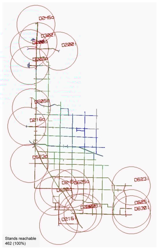
Figure 1. Depot locations with a maximum 15 min wait time for passengers.

Together, these modules allowed the simulation to more realistically model the operational conditions of a flexible, hybridised public transport network, where vehicle dispatch and depot siting are not fixed but responsive to spatial and temporal passenger demand.

3.1.4. Simulation Scope and Assumptions

For the purposes of comparative analysis, the spatial and temporal distribution of travel demand is held constant across all scenarios. The network includes fixed public transport routes and stop locations derived from General Transit Feed Specification (GTFS) and smartcard data. Demand-responsive buses operate over the same physical network but are governed by module-driven dynamic logic.

This technical extension of the Commuter framework enables realistic evaluation of hybrid transport scenarios, including scheduled–on-demand transitions, peak–off-peak reallocation, and varying fleet size configurations. Results from these simulation experiments are analysed across multiple performance dimensions in subsequent sections.

3.2. Behavioural Survey Phase

The second component of the methodological framework involved a behavioural survey to capture user preferences, acceptance levels, and mode choice trade-offs associated with potential on-demand public transport services in Melbourne. This phase served two primary objectives: (1) to estimate the likely mode shift toward demand-responsive services under future deployment scenarios, and (2) to provide empirical input for calibrating agent cost parameters and assigning behavioural classes within the simulation model.

3.2.1. Survey Design and Sampling

A SP survey was administered to residents in the inner metropolitan area of Melbourne from July 2020 to March 2021. Respondents were asked about their current travel behaviour, perceptions of service attributes (e.g., waiting time, reliability, price), and willingness to shift to a hypothetical on-demand public transport service if made available.

Out of 510 total responses, 327 met the inclusion criteria for analysis, exceeding the required minimum sample size for 95% confidence ($n=246$). The sample was demographically balanced (54% male, 46% female), with most respondents aged 23–40 years and a high rate of educational attainment (67% university graduates). Travel purposes were predominantly work and education, with 69% of weekday morning trips reported as commuting and 13% as travel to study.

ODPT adoption rates were initially derived from SP responses, with peak-period uptake set at 17% and off-peak at 100%. In order to address potential SP-revealed preference (RP) gaps and the limited, localised sample, utility-based formulations were implemented using a multinomial logit framework. The travel mode utility incorporates travel time, wait time, walking distance, cost, and service reliability, producing mode choice probabilities that reflect realistic trade-offs. These probabilities were directly integrated into the agent-based simulation, determining the mode shifts of travellers under each scenario.

Sensitivity analyses were conducted by varying key utility parameters (e.g., value of time, wait-time penalties, perceived service reliability) to assess the robustness of predicted adoption rates. Results indicate that while absolute uptake varies with parameter adjustments, the relative performance ranking of scenarios remains stable, supporting the robustness of comparative evaluations.

A larger and more geographically diverse sample would improve representativeness and the precision of utility estimates. Future research could extend this framework using mixed logit or nested logit models to better capture individual heterogeneity and correlation between alternatives, enhancing behavioural realism in scenario analyses.

3.2.2. Key Attributes and Preferences

The survey instrument included SP choice tasks presenting trade-offs between scheduled and on-demand services, varying by travel time, crowding, fare, and reliability. Responses revealed that the most important determinants of willingness to use on-demand public transport were

• Reliability and punctuality;
• Waiting time and travel time;
• Crowding levels (seat availability);
• Price competitiveness with regular services;
• Flexibility and directness of service.

Approximately 67% of respondents indicated they would be likely to choose on-demand public transport if it were available with desirable service characteristics. A further 17% stated they would “definitely use it,” suggesting a substantial early adopter segment. Only 17% expressed resistance to switching, preferring to retain their existing mode.

3.2.3. Integration into Simulation Model

Survey results were used to parameterise behavioural rules within the simulation, specifically,

• Estimating the proportion of peak-period users likely to adopt on-demand services under different scenarios.
• Calibrating generalised cost coefficients (e.g., value-of-waiting-time, fare sensitivity) for public transport user agents.
• Assigning user classes with different utility functions based on demographic attributes (e.g., income, flexibility preference).

For Scenario 2, the 17% of peak-hour passengers who expressed certainty in choosing on-demand services were modelled as automatic adopters, while the remaining demand was allocated to scheduled services. For off-peak periods, where respondents showed higher openness to change, the model assumed 100% allocation to on-demand options.

The inclusion of behavioural data enhances the realism and credibility of the scenario evaluations, ensuring that simulated passenger choices are grounded in stated user preferences rather than arbitrary assumptions.

Table 1 summarises key characteristics of the behavioural survey sample and highlights how the results were incorporated into the simulation framework. The survey responses were used not only to estimate potential adoption rates of on-demand services but also to inform the calibration of agent behaviour and utility weighting in the simulation model. The table links each survey finding with its modelling implication, ensuring that passenger heterogeneity and stated preferences are explicitly captured in scenario development.

Table 1. Summary of key survey findings and modelling implications—Prof Dia.

Attribute	Survey Result	Modelling Use
Total valid responses	327 (out of 510)	Exceeds 95% confidence threshold (n = 246)
Gender split	54% male, 46% female	Demographic segmentation for agent class assignment
Age distribution	Predominantly 23–40 years	Calibrates user profiles for working-age commuters
Education level	67% university educated	Higher tech-readiness assumed for mode adoption
Primary travel purpose	69% work, 13% education	Informs peak-period demand scenarios
Likely to use on-demand public transport	67%	Used to define flexible agent type preferences
Definitely would switch	17%	Allocated to on-demand in Scenario 2 (peak)
Strongly opposed	17%	Retained in scheduled public transport category
Top service attributes	Reliability, wait time, cost, crowding	Used to calibrate generalised cost function coefficients

The survey results provided strong support for the potential uptake of on-demand public transport, with over two-thirds of respondents indicating a willingness to adopt such services if key service features were met. Notably, 17% of users stated they would “definitely switch,” which justifies the modelling assumption in Scenario 2 where this proportion of peak-period demand is allocated to on-demand services.

The demographic profile, skewed toward young, well-educated, and employed individuals, suggests a user base that is digitally literate and likely to value convenience and flexibility. This informed the behavioural segmentation of simulation agents and supports the use of dynamic cost weighting and route choice logic that prioritises service reliability and lower perceived wait times.

Furthermore, the importance placed by users on service reliability, reduced crowding, and waiting time aligns with the structural advantages of on-demand systems and reinforces the relevance of performance indicators used in the comparative evaluation. The integration of these behavioural insights into the agent-based simulation enhances the model’s behavioural realism and policy relevance.

3.3. Demand Prediction Phase

The third component of the modelling framework involved developing a short-term demand forecasting model to support real-time dispatch of on-demand public transport services. Predicting short-interval passenger demand is critical for ensuring efficient vehicle allocation, especially in systems where fleet size, depot location, and vehicle dispatch frequency are dynamically optimised.

3.3.1. Model Objective and Setup

The goal was to forecast future passenger boardings at 15 min, 30 min, and 60 min horizons for a subset of high-frequency bus routes in inner Melbourne. Forecasts were used to inform vehicle dispatch schedules and expected service levels at each stop.

Let $x_t$ represent the observed number of passengers boarding at time step t, and ${\widehat{x}}_{t+\tau }$ the predicted boarding count at a future time $t+\tau$, where $\tau \in \{15,30,60\}$ minutes. The forecasting task was formulated as a sequence-to-sequence time series prediction problem:

$${\widehat{x}}_{t+\tau }=f(x_t,x_{t-1},\dots ,x_{t-n};\theta )$$

(3)

where f is the forecasting model (a BiLSTM neural network), and $\theta$ denotes the learned parameters. The input to the model is a sliding window of past demand observations, which the model uses to predict future values over the specified horizons.

3.3.2. Data Sources and Feature Engineering

The dataset consisted of smartcard tap-on records for 18 high-frequency bus routes covering 1781 unique stops, collected over a one-month period (May 2018). Records were aggregated into 15 min intervals to produce univariate time series of the form $\left\{x_t\right\}$.

  Input features included

• Past passenger count per stop;
• Hour-of-day and day-of-week indicators (modelled as cyclical variables);
• Lagged rolling averages of past demand.

All features were standardised to zero mean and unit variance before model training. The data were split into training (70%), validation (15%), and test (15%) sets. Separate models were trained for each route to capture route-specific demand patterns and spatial heterogeneity.

3.3.3. Model Architecture and Training

The BiLSTM model was selected for its ability to capture temporal dependencies in both forward and backward directions, enhancing short-term demand prediction compared to unidirectional Long Short-Term Memory (LSTM), Gated Recurrent Unit (GRU) or Temporal Convolutional Network (TCN) models. Input features included sliding windows of 15 min intervals over the preceding hours, as well as day-of-week and time-of-day indicators to account for seasonal patterns. Separate models were trained for each route to reflect route-level heterogeneity. Overfitting was mitigated using dropout layers, early stopping, and cross-validation, with hyperparameters tuned via grid search to optimise predictive performance.

LSTM models are a form of recurrent neural network (RNN) designed to handle sequential data by retaining long-term dependencies. The bidirectional extension processes the sequence both forwards and backwards, enabling the model to learn patterns from both past and future temporal context.

The network architecture consisted of

• Input Layer: sequence length of 96 (corresponding to 24 h of 15 min intervals);
• BiLSTM Layer: 300 hidden units in each direction (forward and backward);
• Concatenation Layer: merges the forward and backward hidden states;
• Dense Layer: a fully connected output layer that maps the concatenated hidden state to a scalar prediction;
• Loss Function: Mean Squared Error (MSE);
• Optimiser: Adaptive Moment Estimation (Adam) with a learning rate of 0.001.

The functional form of the model can be expressed as

$$\mathrm{BiLSTM}\left(x_t\right)=\overrightarrow{h_t}\oplus \overleftarrow{h_t}$$

(4)

$${\widehat{x}}_{t+\tau }=\mathrm{Dense}\left([\overrightarrow{h_t},\overleftarrow{h_t}]\right)$$

(5)

Here, $\overrightarrow{h_t}$ and $\overleftarrow{h_t}$ denote the hidden states from the forward and backward passes, respectively, and ⊕ denotes concatenation. The concatenated vector is passed through a Dense layer (i.e., a fully connected layer), which produces a scalar output representing the predicted passenger count. The model is trained using the Adam optimiser, which adaptively adjusts learning rates during training to accelerate convergence and improve generalisation.

3.3.4. Evaluation and Application

Model performance was evaluated using Mean Absolute Percentage Error (MAPE) and Root Mean Squared Error (RMSE) on the test dataset. Across the evaluated routes, the BiLSTM models achieved over 90% accuracy for 15 min forecasts and maintained robust predictive accuracy at longer horizons (30 and 60 min). Forecasts were then fed into the Dynamic Dispatch Scheduling module of the simulation model to inform vehicle release timing and capacity matching.

This predictive component enables the broader simulation framework to incorporate realistic temporal variability in demand and supports proactive dispatch of vehicles in response to short-term demand fluctuations.

3.3.5. Results and Model Performance

The BiLSTM model outperformed five benchmark models, including AutoRegressive Integrated Moving Average (ARIMA), Prophet, feed-forward Artificial Neural Network (ANN), unidirectional LSTM, and GRU, across all prediction horizons. Key accuracy metrics included

• Mean Absolute Percentage Error (MAPE): 1.7–4.3% across all stops;
• Coefficient of Determination ($R^2$): consistently greater than 0.92;
• Root Mean Squared Error (RMSE): route-dependent but stable across time periods.

The model was especially effective at capturing morning and evening peak demand variations, which are critical for time-sensitive vehicle dispatch scheduling in high-frequency corridors.

3.3.6. Integration with Simulation Framework

Forecasted demand values ${\widehat{x}}_{t+\tau }$ were used by the Dynamic Dispatch Scheduling module to determine

• The number of vehicles to dispatch from each depot at each time interval;
• The fleet type (4-, 7-, or 12-seat vehicles) based on aggregated demand thresholds;
• The departure intervals, replacing fixed headways with predicted demand-driven schedules.

This predictive layer ensures that service frequency dynamically adapts to anticipated demand, reducing both passenger wait times and fleet idle time. The result is improved user experience and operational efficiency.

Figure 2 illustrates the full architecture of the demand prediction and simulation integration process. The diagram shows how smartcard and GTFS data are transformed into real-time demand forecasts using a BiLSTM model, which are then ingested by the simulation engine to inform dynamic vehicle dispatch, route allocation, and schedule adaptation.

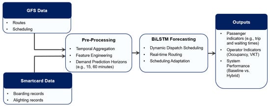
Figure 2. BiLSTM demand prediction pipeline integrating short-term passenger forecasting with simulation-based vehicle dispatch and service scheduling.

As shown in Figure 2, the pipeline enables predicted passenger volumes to influence simulation inputs at multiple levels, including the number and type of vehicles dispatched, time-varying schedules, and depot allocation strategies. By embedding the BiLSTM model into the simulation framework, the system supports responsive, data-driven fleet management aligned with real-world demand dynamics.

3.4. Modelling Public Transport Services

This study models two distinct modes of public transport operations: conventional fixed-route, fixed-schedule services, and demand-responsive on-demand bus services. Both modes are implemented within the agent-based simulation framework using route, stop, and timetable data, augmented with demand- and behaviour-specific logic for each operational scenario.

3.4.1. Scheduled Bus Services

Scheduled buses operate along pre-defined routes and timetables derived from GTFS datasets provided by Public Transport Victoria. Each service includes the following components:

• Stops: Represented as fixed public transport stands, where passengers can board or alight.
• Trails: Sequences of road links specifying vehicle paths between stops.
• Timetables: Fixed departure times by route and direction.
• Vehicle characteristics: 43-seat diesel buses, with constant dwell times (15–30 s) and fixed headways during peak and off-peak periods.

Passenger agents dynamically choose their boarding stops and routes based on generalised cost functions (see Section 3.3), with access and egress segments modelled as walking.

3.4.2. On-Demand Bus Services

In contrast, on-demand buses are modelled as dynamic services that depart in response to short-term passenger demand forecasts generated by the BiLSTM model (Section 3.3). These services share the same physical network and stop locations as the scheduled services but differ in their vehicle assignment, dispatch logic, and boarding rules.

• Fleet Types: Vehicles with capacities of 4, 7, or 12 passengers are assigned based on aggregate stop-level demand within each time window.
• Dispatch Timing: Vehicles are released at irregular intervals determined by forecasted demand ${\widehat{x}}_{t+\tau }$. Departure intervals vary between 5 and 20 min, depending on stop-level boarding thresholds.
• Dwell Logic: Dwell times are dynamically assigned based on actual boarding/alighting activity.
• Routing Flexibility: All vehicles follow pre-defined trails but may skip intermediate stops with no predicted demand.

3.4.3. Skipped Stop Logic

To increase operational efficiency, the simulation enables conditional skipping of bus stops by on-demand vehicles. For a vehicle assigned to a route segment, let

• $s_i$ be a candidate stop;
• $d_{s_i}$ be the forecasted demand at stop $s_i$ during dispatch interval $\tau$;
• $\theta$ be a minimum demand threshold (e.g., one passenger).

The stop is skipped if the forecasted demand falls below the threshold, as defined in Equation (6):

$$\mathrm{Skip}\left(s_i\right)=\left\{\begin{array}{cc}1\hfill & \mathrm{if}{d}_{s_i}<\theta \hfill \\ 0\hfill & \mathrm{otherwise}\hfill \end{array}\right.$$

(6)

This logic is implemented via the simulation’s conditional event framework, improving average travel times and vehicle occupancy rates.

3.4.4. Passenger–Vehicle Assignment

Passenger agents are matched to vehicles based on spatial proximity and earliest service availability, considering walking access and waiting cost. For on-demand services, if multiple vehicles are eligible within a time window, assignment is made to minimise generalised cost $C_{ij}$ as defined in Section 3. Vehicle assignment respects fleet capacity constraints, and excess demand triggers additional dispatch events or delays.

3.4.5. Multi-Stage Journey Handling

Both fixed-route and on-demand public transport services are modelled as part of full multi-stage journeys, including walking access/egress and transfer segments. The simulation handles these as chained agent actions, with consistent cost functions and behavioural rules applied across segments. If a journey includes access by car, a parking cost and walk-to-platform segment is appended, maintaining realism in multi-modal trip chains.

3.4.6. Simulation Scenario Integration

The full-day simulation covers 25 h (including warm-up and cool-down periods) and includes three operational scenarios:

• Baseline: All services operated by scheduled buses with fixed routes and timetables.
• Scenario 1: Scheduled buses for peak periods; on-demand services for off-peak periods.
• Scenario 2: Mixed services during peak (17% shift to on-demand); on-demand only for off-peak periods.

Public transport service performance under each scenario is analysed across key performance indicators (KPIs) including average trip time, occupancy, emissions, and operational cost (see Section 5).

Figure 3 presents a comparative overview of the operational logic and structural components of scheduled and on-demand bus services as implemented in the simulation model. While both services operate on a shared road network and use common infrastructure elements such as public transport stops and agent-based behavioural rules, they differ substantially in their operational design. Scheduled bus services rely on fixed routes, predetermined stop sequences, and consistent headways using standard 43-seat vehicles. In contrast, on-demand services leverage BiLSTM-based demand forecasts to determine dynamic dispatch timing, vehicle type selection (ranging from 4 to 12 seats), and flexible routing that allows for conditional stop skipping based on predicted demand. Figure 3 visually emphasises this duality: fixed versus adaptive scheduling, homogeneous versus heterogeneous fleet composition, and rigid versus responsive service logic. Together, these distinctions illustrate how the hybrid simulation framework integrates both traditional and innovative public transport paradigms to assess system-wide impacts under varying operational scenarios.

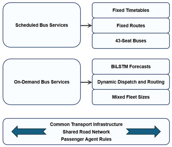
Figure 3. Comparison of scheduled and on-demand bus services: service logic, vehicle configurations, and shared simulation infrastructure.

Table 2 summarises the operational differences between scheduled and on-demand bus services as implemented in the simulation. The contrast spans service design, routing logic, dispatch frequency, and vehicle configuration, reinforcing the model’s capacity to evaluate hybrid and flexible systems in detail.

Table 2. Operational comparison of scheduled vs. on-demand public transport services.

Aspect	Scheduled Bus Services	On-Demand Bus Services
Dispatch Logic	Fixed timetable	Dynamic, demand-driven (via BiLSTM forecasts)
Routing	Fixed routes and stop sequences	Flexible routing with skipped stops when demand $<\theta$
Vehicle Type	43-seat standard buses	Mixed fleet (4-, 7-, 12-seat vehicles)
Departure Interval	Regular headways	Irregular, varies with predicted demand
Passenger Assignment	Predefined service schedules	Real-time assignment based on generalised cost minimisation
Dwell Time	Fixed (15–30 s)	Dynamic, based on actual boarding/alighting
Stop Logic	All stops served regardless of demand	Stops skipped if no demand forecasted ($d_{s_i}<\theta$)
Integration in Simulation	Fixed trip tables	Module-based dispatch and depot assignment logic

4. Scenario Design and Experimental Setup

This section describes the empirical context, data sources, and operational scenarios developed to evaluate the performance of on-demand public transport services in Melbourne. The simulation is designed to compare fixed-route and hybrid on-demand configurations using consistent travel demand inputs and a calibrated microsimulation model.

4.1. Study Area and Network Coverage

The simulation network covers a 35.3 km² area in inner Melbourne, Australia, selected for its high trip density and multimodal connectivity. The study area includes

• 134 signalised intersections;
• 18 public bus routes (36 inbound/outbound);
• 462 bus stops;
• Major arterial corridors with congestion-sensitive flow.

Figure 4 displays the geographic distribution of bus stops and their passenger volumes, with symbol size proportional to daily boardings.

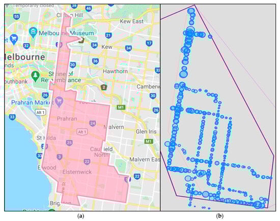
Figure 4. (a) Selected study area. (b) Bus stop locations within the study cordon area. Source: Authors. Produced using Java version 8 in Eclipse IDE.

4.2. Data Sources

The model integrates multiple data sources, including

• Smartcard data from Public Transport Victoria (PTV) covering approximately 225,548 valid passenger trips;
• GTFS static data on routes, stops, and timetables;
• SCATS signal timing plans for intersection control logic;
• VISTA travel survey data for background private vehicle trips;
• Behavioural survey data (see Section 3) for preference segmentation;
• BiLSTM demand forecasts (Section 3.3) for short-term passenger volume prediction.

These integrated datasets ensure realistic modelling of both travel behaviour and network performance. Table 3 summarises the key data sources, their origins, temporal coverage, and specific modelling roles. All datasets were cleaned and aligned to common spatial and temporal formats, with invalid entries, school buses, and through-trips excluded.

Table 3. Overview of data sources used for simulation and model development.

Data Type	Source	Description and Use	Year
Passenger Demand (Smartcard)	Public Transport Victoria (PTV)	Weekday bus trip records (touch-on/off); OD matrix estimation and route-level passenger volumes	2018
Behavioural Survey	Authors’ SP survey	Mode choice preferences, reliability/cost trade-offs, likely uptake of on-demand services	2020–2021
Background Traffic Volumes	VISTA Survey	Private vehicle OD matrix for background congestion simulation	2018
Public Transport Routes & Stops	GTFS + Aerial Imagery	Geographic data on route alignments and stop locations	2018
Traffic Signal Control	SCATS	Signal phase plans and intersection geometry for micro-level control modelling	2018
Demand Forecasting Inputs	Smartcard + Temporal Features	Input data for BiLSTM demand prediction models (aggregated to 15 min intervals)	2018

The integration of operational data (e.g., GTFS, SCATS) with demand-side data (smartcard and behavioural surveys) ensures that both network conditions and passenger decision-making are faithfully represented. The temporal alignment of all data to the 2018 base year enables consistent calibration, while growth-adjusted scaling (Section 3) allows the simulation to reflect pre-COVID-19 demand conditions expected in 2019.

Table 4 details the observed smartcard-based passenger volumes across the 18 routes within the study area. Trips are classified by origin–destination geography relative to the simulation cordon. This route-level distribution was used as the baseline demand input across all three service scenarios and provided benchmarks for model validation.

Table 4. Weekday passenger trip distribution by route and direction.

Route	IN–IN 1	IN–OUT 2	OUT–IN 3	Total Trips
Route 200	1151	6891	6070	14,112
Route 207	1353	7348	6065	14,766
Route 216	2052	1389	1614	5055
Route 219	2607	1572	1208	5387
Route 220	6868	3584	2468	12,920
Route 246	65,541	0	0	65,541
Route 302	106	2176	2152	4434
Route 304	73	1690	1530	3293
Route 305	19	1023	841	1883
Route 309	17	483	748	1248
Route 350	98	1273	1144	2515
Route 605	5711	3605	2122	11,438
Route 623	3199	4904	4554	12,657
Route 625	2688	2129	1789	6606
Route 630	10,464	14,434	12,563	37,461
Route 905	111	3511	3761	7383
Route 906	124	3531	4291	7946
Route 907	141	5028	5734	10,903
Total	102,323	64,571	58,654	225,548

¹ IN–IN: both origin and destination within the study area; ² IN–OUT: origin inside, destination outside; ³ OUT–IN: origin outside, destination inside.

4.3. Scenario Configuration

To evaluate the operational and performance implications of integrating on-demand public transport (ODPT) services, three simulation scenarios were developed. These configurations were designed to reflect realistic implementation stages and are all based on the same origin–destination matrix derived from smartcard data to ensure comparability. Table 5 summarises the operational logic applied in each scenario, including peak and off-peak service differentiation, vehicle types, and the level of on-demand integration.

Table 5. Operational scenario descriptions.

Scenario	Description
Baseline	Only scheduled buses operate using fixed routes, timetables, and 43-seat vehicles.
Scenario 1	Scheduled buses operate during peak hours (7–9 AM, 3–6 PM); on-demand buses operate off-peak.
Scenario 2	Mixed-mode peak period: 17% of passengers use on-demand buses (based on survey data); 83% use scheduled buses. Off-peak is fully serviced by on-demand vehicles.

These three scenarios represent progressively higher levels of on-demand service integration. The baseline reflects existing operations and serves as a performance benchmark. Scenario 1 simulates a transitional model, maintaining scheduled buses during high-demand periods while shifting to demand-responsive services in off-peak windows. Scenario 2 represents a hybrid configuration, incorporating on-demand flexibility even during peak hours based on observed user preferences. This design allows the simulation to capture the potential system-wide benefits of ODPT without requiring full replacement of existing services.

Fleet types for on-demand services in Scenarios 1 and 2 include 4-, 7-, and 12-seat vehicles. Fleet assignment is governed by stop-level BiLSTM demand forecasts and minimum dispatch thresholds.

Table 6 summarises the total number of transport services modelled in each scenario across peak and off-peak periods. These values reflect differences in fleet deployment strategies, with Scenarios 1 and 2 using mixed fleets and dynamic dispatching for on-demand services.

Table 6. Number of scheduled and on-demand services by time period and scenario.

Scenario	Morning Peak (7:00–9:00)	Evening Peak (15:00–18:00)	Off-Peak (Other Hours)	Total Services
Baseline	271	358	1075	1704
Scenario 1	271 (scheduled)	358 (scheduled)	1299 (on-demand)	1928
Scenario 2	291 (mixed)	390 (mixed)	1301 (on-demand)	1982

Compared to the baseline scenario, Scenarios 1 and 2 show increased total service counts due to the deployment of smaller, more frequent on-demand vehicles during off-peak hours. In Scenario 2, modest increases in peak-period services reflect the partial mode shift (17%) from scheduled to on-demand services, consistent with behavioural survey findings. These operational changes form the basis for comparative evaluation in the next section.

4.4. Demand Estimation and Temporal Scaling

To estimate pre-COVID-19 travel conditions, a growth factor of 1% per annum was applied to the 2018 smartcard dataset, consistent with BITRE estimates for Melbourne. This scaled the weekday passenger trip volume from 10,108 to 10,209 trips, which was used as the base demand for the simulation.

Passenger demand was disaggregated into 15 min intervals and fed into the BiLSTM forecasting model for short-term prediction. These predictions informed both

• Fleet composition by time window (e.g., small vs. medium vehicles);
• Depot-level dispatch scheduling with 15 min response time (see Section 3).

To ensure simulation stability, a 25 h model run was used (00:00–01:00 the following day), incorporating warm-up and cool-down periods. Demand matrices for private vehicles were generated using VISTA data and applied to simulate background traffic volumes under typical weekday conditions.

Figure 5 illustrates the total weekday passenger trip distribution by hour. Two distinct peak periods are evident: a morning peak from 7:00 to 9:00 AM, and an afternoon peak from 3:00 to 6:00 PM. These temporal characteristics informed the segmentation of simulation scenarios (see Section 3) and the BiLSTM forecasting intervals used to optimise fleet scheduling. The steep rise and fall in demand during peak hours further justified the simulation of flexible dispatch strategies combining scheduled and on-demand services.

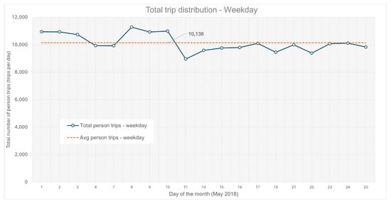
Figure 5. Bus passenger trip distribution by hour (weekday totals based on smartcard data).

Figure 6 provides a 15 min interval breakdown of morning and afternoon demand. The AM peak reaches its maximum between 8:00 and 8:30 AM, while the PM peak shows a broader plateau from 3:30 to 5:30 PM. These temporal profiles were used to configure vehicle dispatch intervals and assign vehicle types under Scenarios 1 and 2. They also validated the use of BiLSTM models to capture short-term demand fluctuations, improving responsiveness and operational efficiency in the agent-based simulation.

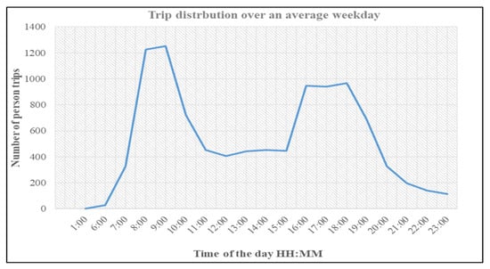
Figure 6. Temporal passenger demand profiles for AM and PM peak periods, based on 15 min smartcard data aggregation.

4.5. Scenario Evaluation Objectives

The three simulation scenarios were evaluated to address the following research questions:

• How do hybrid on-demand configurations affect average passenger travel times and waiting times?
• What is the impact on vehicle occupancy and emissions per passenger trip?
• Can small on-demand fleets provide operational cost advantages in off-peak periods?
• How well do depot placement and forecast-based dispatch algorithms meet spatial demand coverage?

Results are presented in Section 5 and evaluated across six key performance indicators (KPIs): travel time, wait time, occupancy, emissions, fleet distance, and cost per trip.

Table 7 summarises the total number of transport services modelled under each scenario, disaggregated by time period.

Table 7. Summary of transport services by scenario and time period.

Scenario	Morning Peak	Evening Peak	Off-Peak	Total Services
Baseline	271	358	1075	1704
Scenario 1	271	358	1299	1928
Scenario 2	291	390	1301	1982

5. Results and Evaluation

5.1. Model Validation

Model validation was conducted in two parts:

• Comparison of simulated and observed passenger travel times.
• GEH analysis of route-level passenger volumes during peak periods.

Figure 7 shows the distribution of modelled versus observed weekday passenger travel times across all routes in the study area. The simulation results closely match observed data from smartcard records, with the highest agreement in the 10–30 min range where most trips occur. Minor deviations appear at the tails of the distribution, with short trips (<10 min) slightly under-represented and long trips (>40 min) modestly over-represented. This indicates that the simulation accurately captures the central tendency of trip durations.

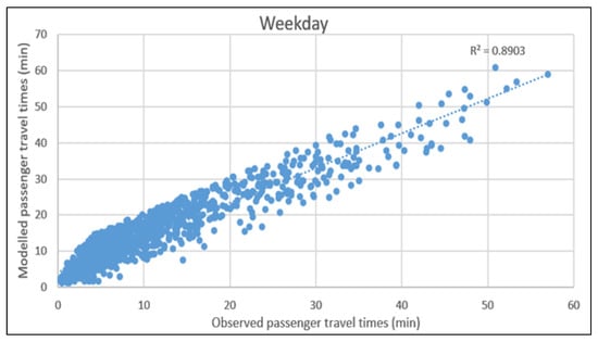
Figure 7. Modelled versus observed passenger travel times for average weekdays.

Table 8 presents GEH statistics comparing modelled and observed passenger volumes during the AM and PM peak hours. GEH values below 5 are generally considered acceptable for model validation. The average GEH across periods was 3.3 (AM) and 3.6 (PM), with most routes within acceptable bounds, supporting the validity of the simulation results.

Table 8. GEH values for AM and PM peak periods.

Peak Period	GEH Value
Morning Peak (7:00–8:00)	0.28
Morning Peak (8:00–9:00)	0.39
Evening Peak (16:00–17:00)	0.29
Evening Peak (17:00–18:00)	0.32

5.2. Scenario Evaluation Results

This section presents comparative results for the three scenarios defined in Section 3, evaluated across six key performance indicators (KPIs):

• Average passenger travel time (minutes);
• Average passenger waiting time (minutes);
• Vehicle occupancy rate (passengers per vehicle);
• Total fleet distance travelled (km);
• Emissions per passenger trip (kg CO₂-e);
• Service cost per passenger (AUD, estimated).

5.2.1. Travel Time and Wait Time

Figure 8 shows that both Scenario 1 and Scenario 2 reduced average passenger trip times compared to the baseline. Scenario 2 achieved the greatest improvement, with a 26% reduction in travel time during the AM peak and 32% during the PM peak. Wait times followed a similar pattern, declining by 20–35%, particularly in off-peak periods where on-demand services replaced infrequent scheduled services.

Figure 8. Average passenger travel time and wait time by scenario and time period.

5.2.2. Vehicle Occupancy and Fleet Efficiency

Scenario 2 delivered a substantial increase in average vehicle occupancy, reaching levels up to three times higher than the baseline for small on-demand vehicles during off-peak periods. Fleet kilometres travelled increased marginally due to higher service frequency, but occupancy gains offset these increases in terms of system efficiency.

5.2.3. Emissions and Environmental Impact

Total emissions per passenger trip declined significantly in Scenarios 1 and 2 due to improved load factors and smaller vehicle sizes. Scenario 2 recorded a 72% reduction in emissions per passenger on an average weekday compared to the baseline.

5.2.4. Operational Costs

While on-demand services entail higher dispatch and coordination complexity, estimated per-passenger service costs declined in both hybrid scenarios. This was attributed to improved vehicle utilisation and reduced idle times. Scenario 2 achieved the best cost-efficiency during off-peak periods.

5.2.5. Summary of Performance Trade-Offs

Table 9 provides a summary of all six KPIs across the three simulation scenarios. Scenario 2 consistently outperformed the baseline and Scenario 1 in most indicators, suggesting that a hybrid model combining scheduled and on-demand services can improve performance across user, operator, and environmental dimensions.

Table 9. Summary of scenario performance across key indicators.

Performance Indicator	Baseline	Scenario 1	Scenario 2
Average travel time (min)	36.0	30.1	26.6
Average wait time (min)	10.2	7.8	6.5
Vehicle occupancy (pax/veh)	12.1	15.7	18.6
Fleet distance travelled (km)	17,102	18,234	18,667
Emissions per trip (kg CO2-e)	2.21	0.92	0.62
Service cost per trip (AUD)	6.82	5.11	4.73

5.3. Passenger Service Quality and Trip Experience

Passenger-level service outcomes were assessed using four key indicators:

• Average passenger distance travelled (km);
• Average walk time (min);
• Average wait time (min);
• Average total trip duration (min).

Table 10 summarises the performance of each simulation scenario against these indicators.

Table 10. Passenger service quality indicators by scenario.

Indicator	Baseline	Scenario 1	Scenario 2
Average Passenger Distance (km)	5.6	5.6	5.6
Average Passenger Walk Time (min)	6.2	6.2	6.2
Average Passenger Wait Time (min)	9.6	6.6	6.3
Average Passenger Trip Duration (min)	41.5	30.6	28.4

The results show that while the average trip distance remained stable across all scenarios (5.6 km), reflecting consistent origin–destination patterns, there were substantial improvements in time-based service quality metrics under the on-demand scenarios.

In terms of passenger wait time, Scenario 1 reduced the average from 9.6 to 6.6 min (a 31% improvement), while Scenario 2 achieved an even greater reduction to 6.3 min (34% improvement). These gains are attributed to more frequent service dispatches during off-peak periods and dynamic routing that reduced vehicle idle time and improved responsiveness.

Passenger trip duration showed the most significant improvement, decreasing from 41.5 min in the baseline to 30.6 min in Scenario 1 (a 26% reduction) and to 28.4 min in Scenario 2 (a 32% reduction). These improvements were driven by the ability of on-demand services to offer more direct routing and eliminate unnecessary stops through demand-driven logic.

Interestingly, walk times remained constant across all scenarios at 6.2 min. This suggests that on-demand services maintained equitable access to bus stops or smart stops, without introducing additional walking burdens on passengers. It also indicates that system accessibility was preserved despite changes in operational configuration.

Together, these results demonstrate that on-demand service integration significantly enhances the passenger experience, particularly by reducing wait and trip times without compromising accessibility or travel distance.

5.4. System and Operator Efficiency

System-level efficiency and operational productivity were assessed using three key metrics:

• Total passenger completions;
• Total completed transport distance;
• Transport completion ratio (passenger completions per kilometre travelled).

The results show that Scenario 2 consistently outperformed the baseline and Scenario 1, particularly during the AM peak. Passenger completions increased from 40,373 in the baseline to 44,945 in Scenario 2, representing an 11% uplift in completed trips. During the PM peak, completions remained steady at around 51,000 for Scenario 2—slightly above both the baseline and Scenario 1.

This increase in passenger throughput was achieved despite a moderate rise in total vehicle kilometres travelled, which rose by 30% during the AM peak (from 3427 km in the baseline to 4428 km in Scenario 2). However, this increase was accompanied by a greater proportional rise in trip completions, resulting in a net improvement in the transport completion ratio, which fell from 11.8 in the baseline to 10.2 in Scenario 2 for the AM peak. A lower transport completion ratio indicates greater system efficiency—that is, more passengers served per kilometre of service.

Table 11 summarises the system-level metrics for each scenario, including total completions, transport distance, and the transport completion ratio. These indicators offer insight into operational efficiency and service productivity across time periods.

Table 11. System-level efficiency and operational productivity.

Indicator	Baseline	Scenario 1	Scenario 2
Passenger Completions (AM Peak)	40,373	42,503	44,945
Passenger Completions (PM Peak)	50,598	51,702	51,430
Completed Transport Distance (AM Peak, km)	3427	3905	4428
Completed Transport Distance (PM Peak, km)	4171	4311	4373
Transport Completion Ratio (AM Peak)	11.8	10.9	10.2
Transport Completion Ratio (PM Peak)	12.1	12.0	11.8

Scenario 1 offered modest improvements over the baseline, particularly during the PM peak. However, it was Scenario 2’s fully integrated, mixed-fleet operation that yielded the most substantial gains, largely due to its flexibility in matching vehicle deployment to real-time demand conditions and geographic trip density.

These findings support the use of dynamic on-demand operations to enhance not only passenger outcomes but also system-level throughput and vehicle utilisation. For operators, this translates to better fleet productivity, with reduced dead running and more efficient use of vehicle capacity.

5.5. Environmental Performance

Environmental performance was evaluated by estimating average emissions per completed passenger trip, focusing on three pollutants:

• Carbon dioxide (CO₂);
• Nitric oxide (NO);
• Particulate matter (PM₁₀).

Table 12 presents the average per-trip emissions across all scenarios. The baseline scenario, which relies entirely on conventional scheduled buses, produced the highest emissions levels, with an average of 551.7 g of CO₂ per passenger trip, 1.63 g of NO, and 0.054 g of PM₁₀. These values reflect low occupancy rates and limited vehicle optimisation.

Table 12. Environmental performance indicators.

Indicator	Baseline	Scenario 1	Scenario 2
Average CO2 Emissions per Passenger Trip (g)	551.7	192.8	153.5
Average NO Emissions per Passenger Trip (g)	1.63	0.55	0.44
Average PM10 Emissions per Passenger Trip (g)	0.054	0.019	0.016

In contrast, both on-demand scenarios demonstrated substantial environmental gains. Scenario 1 reduced CO₂ emissions by 65%, NO by 66%, and PM₁₀ by 65% per passenger trip. These reductions were further amplified in Scenario 2, where CO₂ emissions fell by 72%, and NO and PM₁₀ dropped by 73% and 70%, respectively.

These improvements can be attributed to several factors: more efficient route allocation, dynamic vehicle deployment based on real-time demand, and higher passenger occupancy rates. By reducing the number of low-occupancy, high-emissions trips, the on-demand service model shifts transport supply closer to actual usage, enhancing sustainability.

The environmental benefits observed in Scenario 2 reinforce the value of mixed operational strategies that maximise both service quality and emissions efficiency. As cities face increasing pressure to decarbonise their transport systems, these findings offer actionable insights into how operational design can drive emissions reductions at scale.

5.6. Vehicle Occupancy

Vehicle occupancy is a key indicator of service productivity and system efficiency, particularly for public transport operations seeking to optimise energy use and cost per trip. Higher occupancy rates typically reflect more efficient fleet deployment and greater alignment between service supply and passenger demand. In the context of on-demand operations, occupancy also serves as a proxy for the effectiveness of vehicle dispatching algorithms and stop-level demand responsiveness.

Figure 9 presents the average vehicle occupancy for each scenario during the AM and PM peak periods. These values are calculated and averaged across all services operating within the simulation window.

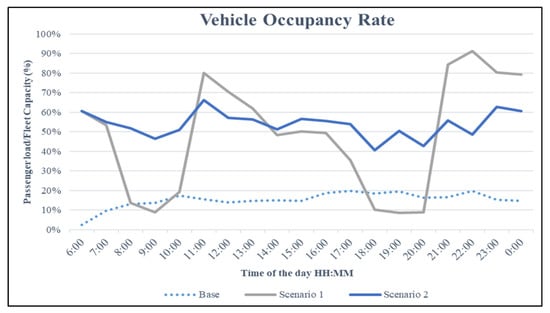
Figure 9. Average vehicle occupancy by scenario during AM and PM peak periods.

Occupancy rates increased substantially in both on-demand scenarios. During the AM peak, the average number of passengers per vehicle rose from 14 in the baseline to 24 in Scenario 1, and further to 42 in Scenario 2. Similarly, PM peak occupancy improved from 16 to 26 in Scenario 1 and 45 in Scenario 2.

These increases are attributed to more effective trip bundling and dynamic fleet management enabled by the on-demand service logic. The flexible deployment of vehicles and real-time routing ensured that vehicles were dispatched in areas of higher passenger concentration, improving load factors and reducing low-occupancy trips.

This trend supports the conclusion that on-demand services not only enhance user experience but also deliver measurable operational benefits to service providers. Higher occupancy directly contributes to lower emissions per passenger, improved cost-efficiency, and better vehicle utilisation.

5.7. Wait Time Performance

Passenger wait time is a critical factor affecting satisfaction and perceived reliability of public transport systems. While scheduled services offer predictable intervals, they often lead to long off-peak waiting periods. In contrast, on-demand services aim to minimise wait times by dispatching vehicles in response to real-time demand.

Figure 10 illustrates the comparison between expected and actual passenger wait times across a sample of five stops in Scenario 2. These stops represent a cross-section of travel demand zones within the study area.

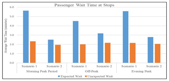
Figure 10. Expected vs. actual passenger wait time by stop (Scenario 2).

Across all stops, the actual wait time was consistently below the pre-defined threshold of 8 min. Most values ranged between 5.9 and 7.0 min—10–20% shorter than expectations. These gains were enabled by flexible dispatch timing and dynamic route generation based on demand profiles and the real-time routing module developed for this study.

Shorter, more predictable wait times improve user perception, reduce uncertainty, and encourage mode shift from private cars—especially in areas underserved by conventional routes. These results validate the model’s behavioural assumptions and its capacity to meet time-based expectations with user-centric design.

5.8. Economic Evaluation and Cost–Benefit Analysis

To assess the financial viability of on-demand public transport services, a simplified economic evaluation was conducted. The analysis draws on cost assumptions and benefit categories from NSW government guidelines, estimating trip-level costs, capital and operating costs, and benefit–cost ratios (BCRs) under peak-period operations.

5.8.1. Estimated Cost per Trip

Table 13 shows the average cost per passenger trip during AM and PM peaks. Scenario 2 achieves the lowest cost in both cases, reducing costs from $2.18 to $1.63 in the morning and from $2.03 to $1.53 in the evening. These gains are attributed to higher occupancy and better fleet utilisation.

Table 13. Estimated cost per passenger trip (AM and PM peak).

Scenario	AM Peak ($AUD)	PM Peak ($AUD)
Baseline	2.18	2.03
Scenario 1	1.76	1.61
Scenario 2	1.63	1.53

5.8.2. Economic Parameters and Assumptions

Table 14 summarises the key inputs used to estimate costs and monetised benefits. Values are drawn from publicly available appraisal manuals, including NSW transport and Australian Treasury guidelines.

Table 14. Economic parameters used in cost–benefit analysis.

Parameter	Value
Capital Cost of Fleet (per bus)	$330,000
Operating Cost per kilometre	$1.50
Value of Travel Time (per hour)	$18.50
Emissions Cost per gram CO2	$0.0001
Discount Rate	7%

5.8.3. Summary of Benefits, Costs, and BCRs

Table 15 summarises the transport indicators used to estimate the economic benefits of time savings, fleet utilisation, and emissions reduction.

Table 15. Summary of transport KPI inputs used in economic evaluation.

Indicator	Baseline	Scenario 1	Scenario 2
Average Trip Time (min)	41.5	30.6	28.4
Vehicle Occupancy (passengers/vehicle)	15.0	25.0	43.5
Emissions per Passenger Trip (g CO2)	551.7	192.8	153.5
Vehicle km Travelled	7598	8216	8801

Using these KPIs and the economic parameters from Table 14, the monetised costs and benefits were computed for each scenario. Table 16 shows total estimated costs, benefits, and the resulting benefit–cost ratios.

Table 16. Summary of benefits, costs, and BCRs (AM and PM peak combined).

Scenario	Total Costs ($M)	Total Benefits ($M)	Benefit–Cost Ratio (BCR)
Baseline	1.52	1.23	0.81
Scenario 1	1.46	2.38	1.63
Scenario 2	1.43	2.79	1.95

The results clearly show that Scenario 2 delivers the strongest economic case, with a BCR of 1.95—nearly $2 in benefits for every $1 spent. Scenario 1 also achieves a strong result, while the baseline scenario fails to meet cost-effectiveness thresholds. These findings support integrating ODPT into public transport networks as a cost-efficient strategy to improve service quality, sustainability, and financial performance.

6. Conclusions and Policy Implications

This study introduced and demonstrated a hybrid simulation framework for evaluating on-demand public transport (ODPT) services. By integrating agent-based simulation, deep learning-based demand forecasting, and behavioural survey modelling, the framework enabled a comprehensive assessment of operational, user experience, environmental, and economic performance across three ODPT service scenarios.

The results provide strong empirical evidence in support of integrating on-demand services into existing public transportation networks. Scenario 2, which applied a fully hybrid model combining on-demand and fixed-route operations, outperformed both the baseline and mixed-schedule Scenario 1 on nearly all performance indicators. From a user perspective, the hybrid scenario reduced trip durations by 32% and wait times by 34%, while maintaining equitable walk distances. Operational efficiency improved through better vehicle utilisation, with peak-period occupancy rates tripling and a greater share of passenger demand met. Environmental outcomes were also positive: per-passenger emissions fell by 72% for CO₂ and by more than 70% for NO and PM₁₀.

Importantly, the economic analysis found the hybrid scenario to be cost-effective. The estimated benefit–cost ratio (BCR) of 1.95 indicates a strong return on investment relative to traditional fixed-route operations. Cost per passenger declined by up to 25%, with monetised gains attributed to travel time savings, improved fleet productivity, and emissions reductions. These results are broadly consistent with prior studies on ODPT and demand-responsive transport, which have reported improvements in travel time, vehicle utilisation, and environmental performance when flexible services complement conventional transit, particularly in low-density or off-peak contexts. For example, Alonso González et al. (2018) found that DRT can substantially improve accessibility compared to conventional fixed route services, particularly for underserved origin–destination pairs [4]. Similarly, the authors’ recent simulation study of flexible on-demand bus services in Melbourne showed reductions in travel times of around 30%, increases in vehicle occupancy, and over 70% reductions in emissions per passenger trip compared to fixed schedules [14]. Studies in other contexts, such as Porto, also demonstrate that DRT frameworks can reduce total distance travelled and stop frequency while maintaining service levels [62]. Moreover, advanced optimisation frameworks for connected DRT services report travel time improvements on the order of 14–36% relative to traditional modes [63].

The findings yield several implications for transport planners and policymakers:

• Dynamic ODPT configurations can effectively complement fixed-route services, particularly in off-peak periods or lower-density areas.
• Investment in real-time analytics, demand forecasting, and simulation tools is critical to the design and management of flexible transport systems.
• Hybrid models offer significant potential for improving equity, access, and environmental sustainability in public transport delivery.
• Smart depot siting and adaptive fleet strategies, guided by predictive models, can enhance both user outcomes and operational performance.

More broadly, this research illustrates how combining simulation, AI, and behavioural data can yield an integrated, transferable evaluation framework. As cities explore scalable and user-responsive mobility reforms, this approach provides a replicable pathway to test, compare, and optimise ODPT strategies in real-world networks.

While the framework provides detailed insights into ODPT operations, some limitations must be acknowledged:

• The case study is limited to Melbourne, which may affect the generalisability of results to other urban contexts with different population densities, travel patterns, and transit networks.
• Passenger behaviour was based on survey and smartcard data, which may not capture all variability or future shifts in travel demand.
• Operational cost and emissions estimations rely on modelled assumptions that simplify real-world complexities.
• The agent-based simulation necessarily abstracts some operational details, such as driver behaviour or vehicle breakdowns, which could influence outcomes in practice.

While Scenario 2 demonstrates significant performance improvements in Melbourne, these results may vary in other urban contexts. In high-density cities with frequent fixed-route services, the relative travel time and emissions benefits of on-demand integration may be lower, while in low-density or suburban networks, gains could be significant. Institutional and financial conditions also influence the applicability of these solutions: successful implementation requires adequate digital infrastructure, regulatory support, and funding mechanisms to sustain flexible operations. Future work should evaluate the framework across diverse geographic and operational contexts to better understand scalability and contextual sensitivity.

Future work could address these limitations by applying the framework to different geographic contexts, incorporating multimodal integration and Mobility-as-a-Service platforms, and validating results against more extensive real-world operational data. Such extensions would further strengthen the applicability of hybrid ODPT evaluation for planning and policy decisions.

References

- Chandra, S.; Quadrifoglio, L. A model for estimating the optimal cycle length of demand responsive feeder transit services. Transp. Res. Part B Methodol. 2013, 51, 1–16. [Google Scholar] [CrossRef]
- Chan, N.D.; Shaheen, S.A. Ridesharing in north america: Past, present, and future. Transp. Rev. 2012, 32, 93–112. [Google Scholar] [CrossRef]
- Mulley, C.; Nelson, J.D.; Wright, S. Community transport meets mobility as a service: On the road to a new a flexible future. Res. Transp. Econ. 2018, 69, 583–591. [Google Scholar] [CrossRef]
- Alonso-González, M.J.; Liu, T.; Cats, O.; Oort, N.V.; Hoogendoorn, S. The potential of demand-responsive transport as a complement to public transport: An assessment framework and an empirical evaluation. Transp. Res. Rec. 2018, 2672, 879–889. [Google Scholar] [CrossRef]
- Brake, J.; Nelson, J.D.; Wright, S. Demand responsive transport: Towards the emergence of a new market segment. J. Transp. Geogr. 2004, 12, 323–337. [Google Scholar] [CrossRef]
- Hazan, J.; Lang, N.; Wegscheider, A.K.; Fassenot, B. On-Demand Transit Can Unlock Urban Mobility; Boston Consulting Group: Boston, MA, USA, 2019; Available online: https://www.bcg.com/en-au/publications/2019/on-demand-transit-can-unlock-urban-mobility.aspx (accessed on 20 February 2020).
- Goodwill, J.A.; Carapella, H. Creative Ways to Manage Paratransit Costs; Report; National Center for Transit Research (US): Tampa, FL, USA, 2008. [Google Scholar]
- Linda, S. Can public transport compete with the private car? Iatss Res. 2003, 27, 27–35. [Google Scholar]
- Mageean, J.; Nelson, J.D. The evaluation of demand responsive transport services in europe. J. Transp. Geogr. 2003, 11, 255–270. [Google Scholar] [CrossRef]
- Liyanage, S.; Dia, H.; Abduljabbar, R.; Bagloee, S.A. Flexible mobility on-demand: An environmental scan. Sustainability 2019, 11, 1262. [Google Scholar] [CrossRef]
- Nelson, J.D.; Wright, S.; Masson, B.; Ambrosino, G.; Naniopoulos, A. Recent developments in flexible transport services. Res. Transp. Econ. 2010, 29, 243–248. [Google Scholar] [CrossRef]
- Liyanage, S.; Dia, H. An agent-based simulation approach for evaluating the performance of on-demand bus services. Sustainability 2020, 12, 4117. [Google Scholar] [CrossRef]
- Liyanage, S.; Dia, H. On-demand technologies for public transport: Insights from a melbourne survey. IEEE Open J. Intell. Transp. Syst. 2025, 6, 653–672. [Google Scholar] [CrossRef]
- Liyanage, S.; Dia, H.; Duncan, G.; Abduljabbar, R. Evaluation of the impacts of on-demand bus services using traffic simulation. Sustainability 2024, 16, 8477. [Google Scholar] [CrossRef]
- Liyanage, S.; Dia, H.; Abduljabbar, R.; Tsai, P.-W. Neural Network Approaches for Forecasting Short-Term On-Road Public Transport Passenger Demands; Edward Elgar Publishing: Cheltenham, UK, 2023; pp. 176–220. [Google Scholar]
- Liyanage, S.P. Modelling the Impacts of On-Demand Public Transport. Ph.D. Thesis, Swinburne University of Technology, Melbourne, Australia, 2022. [Google Scholar]
- Atasoy, B.; Ikeda, T.; Ben-Akiva, M.E. Optimizing a flexible mobility on demand system. Transp. Res. Rec. 2015, 2563, 76–85. [Google Scholar] [CrossRef]
- Atasoy, B.; Ikeda, T.; Song, X.; Ben-Akiva, M.E. The concept and impact analysis of a flexible mobility on demand system. Transp. Res. Part Emerg. Technol. 2015, 56, 373–392. [Google Scholar] [CrossRef]
- Mohamed, M.J.; Rye, T.; Fonzone, A. Operational and policy implications of ridesourcing services: A case of uber in London, UK. Case Stud. Transp. Policy 2019, 7, 823–836. [Google Scholar] [CrossRef]
- Narayan, J.; Cats, O.; Oort, N.; Hoogendoorn, S. On the scalability of private and pooled on-demand services for urban mobility in amsterdam. Transp. Plan. Technol. 2021, 45, 2–18. [Google Scholar] [CrossRef]
- Shaheen, S.; Cohen, A. Mobility on Demand (MOD) and Mobility as a Service (MaaS): Early Understanding of Shared Mobility Impacts and Public Transit Partnerships; Elsevier: Amsterdam, The Netherlands, 2020; pp. 37–59. [Google Scholar]
- Shamshiripour, A.; Rahimi, E.; Shabanpour, R.; Mohammadian, A.K. Dynamics of travelers’ modality style in the presence of mobility-on-demand services. Transp. Res. Part C Emerg. Technol. 2020, 117, 102668. [Google Scholar] [CrossRef]
- Alonso-González, M.J.; van Oort, N.; Cats, O.; Hoogendoorn-Lanser, S.; Hoogendoorn, S. Value of time and reliability for urban pooled on-demand services. Transp. Res. Part C Emerg. Technol. 2020, 115, 102621. [Google Scholar] [CrossRef]
- Wang, Z.; Yu, J.; Hao, W.; Chen, T.; Wang, Y. Designing high-freedom responsive feeder transit system with multitype vehicles. J. Adv. Transp. 2020, 2020, 8365194. [Google Scholar] [CrossRef]
- Cats, O.; Wang, Q.; Zhao, Y. Identification and classification of public transport activity centres in stockholm using passenger flows data. J. Transp. Geogr. 2015, 48, 10–22. [Google Scholar] [CrossRef]
- Bennett, T. Keoride: The Future of On-Demand Transport? 2019. Future Cities. Available online: https://www.goget.com.au/blog/keoride-the-future-of-on-demand-transport/ (accessed on 26 August 2024).
- Downer, K. On Demand Transport: Co-Designing Tailored Mobility Solutions. 2018. Available online: https://www.keolisdowner.com.au/a-community-winner-keoride-on-demand-public-transport-service-in-mount-barker-nairne-and-littlehampton-extended-till-june-2022/ (accessed on 26 August 2024).
- Transport for NSW. Keoride Case Study. 2021. Available online: https://www.transport.nsw.gov.au/data-and-research/nsw-future-mobility-prospectus/nsw-future-mobility-case-studies/procurement-as-3 (accessed on 16 December 2025).
- EU Japan Centre. On-Demand Public Transport|Shotl x Odakyu Electric Railway. 2021. Available online: https://www.eu-japan.eu/publications/demand-public-transport-shotl-x-odakyu-electric-railway (accessed on 12 June 2024).
- Pettersson, F. An International Review of Experiences from On-Demand Public Transport Services; k2 Working Paper; Lund University: Lund, Sweden, 2019. [Google Scholar]
- Bridj. Bridj. 2018. Available online: https://www.bridj.com/ (accessed on 30 December 2018).
- Hawkins, A.J. Ford’s On-Demand Bus Service Chariot Is Going out of Business. The Verge. 2019. Available online: https://www.theverge.com/2019/1/10/18177378/chariot-out-of-business-shuttle-microtransit-ford (accessed on 16 December 2025).
- Sulopuisto, O. Why Helsinki’s Innovative On-Demand Bus Service Failed. Eurbanlab. Accelerating Urban Innovations, 2016. [Google Scholar]
- Edwards, D.; Elangovan, A.K.; Watkins, K. Reaching low-density urban areas with the network-inspired transportation system. In Proceedings of the 2012 15th International IEEE Conference on Intelligent Transportation Systems, Anchorage, AK, USA, 16–19 September 2012; IEEE: New York, NY, USA, 2012; pp. 826–831. [Google Scholar]
- Inturri, G.; Giuffrida, N.; Ignaccolo, M.; Pira, M.L.; Pluchino, A.; Rapisarda, A. Testing Demand Responsive Shared Transport Services via Agent-Based Simulations; Springer: Berlin/Heidelberg, Germany, 2018; pp. 313–320. [Google Scholar]
- Frei, C.; Hyland, M.; Mahmassani, H.S. Flexing service schedules: Assessing the potential for demand-adaptive hybrid transit via a stated preference approach. Transp. Res. Part C Emerg. Technol. 2017, 76, 71–89. [Google Scholar] [CrossRef]
- Arentze, T.A.; Molin, E.J.E. Travelers’ preferences in multimodal networks: Design and results of a comprehensive series of choice experiments. Transp. Res. Part A Policy Pract. 2013, 58, 15–28. [Google Scholar] [CrossRef]
- Liyanage, S.; Dia, H. User preferences for on-demand transport in melbourne: Insights from stated preference surveys. In Proceedings of the Australasian Transport Research Forum 2024 Proceedings, Melbourne, Australia, 27–29 November 2024. [Google Scholar]
- Liyanage, S.; Abduljabbar, R.; Dia, H.; Tsai, P.-W. Ai-based neural network models for bus passenger demand forecasting using smart card data. J. Urban Manag. 2022, 11, 365–380. [Google Scholar] [CrossRef]
- Abduljabbar, R.L.; Dia, H.; Tsai, P.-W.; Liyanage, S. Short-term traffic forecasting: An lstm network for spatial-temporal speed prediction. Future Transp. 2021, 1, 21–37. [Google Scholar] [CrossRef]
- Inturri, G.; Giuffrida, N.; Ignaccolo, M.; Pira, M.L.; Pluchino, A.; Rapisarda, A.; D’Angelo, R. Taxi vs. demand responsive shared transport systems: An agent-based simulation approach. Transp. Policy 2021, 103, 116–126. [Google Scholar] [CrossRef]
- Hu, X.; Zhao, L.; Wang, W. Impact of perceptions of bus service performance on mode choice preference. Adv. Mech. Eng. 2015, 7, 1687814015573826. [Google Scholar] [CrossRef]
- Ryley, T.; Stanley, P.; Zanni, A.; Quddus, M.; Enoch, M. An Examination of the Potential Use of Demand Responsive Transport Services. In Proceedings of the Transportation Research Board 93rd Annual Meeting, Washington, DC, USA, 12–16 January 2014. [Google Scholar]
- Giuffrida, N.; Pira, M.L.; Inturri, G.; Ignaccolo, M. Addressing the public transport ridership/coverage dilemma in small cities: A spatial approach. Case Stud. Transp. Policy 2021, 9, 12–21. [Google Scholar] [CrossRef]
- Calabrò, G.; Pira, M.L.; Giuffrida, N.; Inturri, G.; Ignaccolo, M.; Correia, G.H.d.A. Fixed-route vs. demand-responsive transport feeder services: An exploratory study using an agent-based model. J. Adv. Transp. 2022, 2022, 8382754. [Google Scholar] [CrossRef]
- Enoch, M.; Potter, S.; Parkhurst, G.; Smith, M. Intermode: Innovations in Demand Responsive Transport: Final Report; Social Research in Transport (SORT) Clearinghouse: Melbourne, Australia, 2022. [Google Scholar]
- Dia, H.; Gondwe, W.; Panwai, S. A traffic simulation approach to evaluating the benefits of incident management programs. In Proceedings of the 29th Australasian Transport Research Forum, Gold Coast, Australia, 27–29 September 2006. [Google Scholar]
- Scheltes, A.; Correia, G.H.d. Exploring the use of automated vehicles as last mile connection of train trips through an agent-based simulation model: An application to delft, netherlands. Int. J. Transp. Sci. Technol. 2017, 6, 28–41. [Google Scholar] [CrossRef]
- Araldo, A.; Maria, A.D.; Stefano, A.D.; Morana, G. On the importance of demand consolidation in mobility on demand. In Proceedings of the 2019 IEEE/ACM 23rd International Symposium on Distributed Simulation and Real Time Applications (DS-RT), Cosenza, Italy, 7–9 October 2019; IEEE: New York, NY, USA, 2019; pp. 1–8. [Google Scholar]
- Oh, S.; Seshadri, R.; Le, D.-T.; Zegras, P.C.; Ben-Akiva, M.E. Evaluating automated demand responsive transit using microsimulation. IEEE Access 2020, 8, 82551–82561. [Google Scholar] [CrossRef]
- Chen, Y.; Ji, C.; Cai, Y.; Yan, T.; Su, B. Deep reinforcement learning in autonomous car path planning and control: A survey. arXiv 2024, arXiv:2404.00340. [Google Scholar] [CrossRef]
- Zhang, J.; Xu, H.; Liu, D.; Yu, Q. Advancing dynamic emergency route optimization with a composite network deep reinforcement learning model. Systems 2025, 13, 127. [Google Scholar] [CrossRef]
- Diana, M.; Dessouky, M.M. A new regret insertion heuristic for solving large-scale dial-a-ride problems with time windows. Transp. Res. Part B Methodol. 2004, 38, 539–557. [Google Scholar] [CrossRef]
- Quadrifoglio, L.; Dessouky, M.M.; Palmer, K. An insertion heuristic for scheduling mobility allowance shuttle transit (mast) services. J. Sched. 2007, 10, 25–40. [Google Scholar] [CrossRef]
- Tang, Q.; Du, P. Study on accessibility of feeder lines with different geometric shapes. J. Adv. Transp. 2020, 2020, 4040252. [Google Scholar] [CrossRef]
- Lee, E.H.; Kim, K.; Kho, S.-Y.; Kim, D.-K.; Cho, S.-H. Estimating express train preference of urban railway passengers based on extreme gradient boosting (xgboost) using smart card data. Transp. Res. Rec. 2021, 2675, 64–76. [Google Scholar]
- Zhou, J.; Wang, W.; Liu, Z.; Liu, Y. Loading and unloading time estimation based on xgboost for railway freight transport. Railw. Signal. Commun. Eng. 2024, 21, 36. [Google Scholar]
- Autodesk. Mobility Simulator. 2017. Available online: https://help.autodesk.com/view/INFMDR/ENU/?guid=GUID-111318F7-0F27-4194-B933-07935B9A9640 (accessed on 26 August 2024).
- Azalient. Commuter. 2013. Available online: https://forums.autodesk.com/autodesk/attachments/autodesk/509/7483/1/CommuterManual_036.pdf (accessed on 26 August 2024).
- Dia, H.; Cottman, N. Evaluation of arterial incident management impacts using traffic simulation. In IEE Proceedings-Intelligent Transport Systems; IET: Stevenage, UK, 2006; Volume 153, pp. 242–252. [Google Scholar]
- Stirzaker, C.; Dia, H. Evaluation of transportation infrastructure management strategies using microscopic traffic simulation. J. Infrastruct. Syst. 2007, 13, 168–174. [Google Scholar] [CrossRef]
- Melo, S.; Gomes, R.; Abbasi, R.; Arantes, A. Demand-responsive transport for urban mobility: Integrating mobile data analytics to enhance public transportation systems. Sustainability 2024, 16, 4367. [Google Scholar] [CrossRef]
- Kim, T.W.; Chae, M.; Yu, J.W. Optimization and implementation framework for connected demand responsive transit (drt) considering punctuality. Sustainability 2025, 17, 1079. [Google Scholar] [CrossRef]
Disclaimer/Publisher’s Note: The statements, opinions and data contained in all publications are solely those of the individual author(s) and contributor(s) and not of MDPI and/or the editor(s). MDPI and/or the editor(s) disclaim responsibility for any injury to people or property resulting from any ideas, methods, instructions or products referred to in the content. |
© 2025 by the authors. Licensee MDPI, Basel, Switzerland. This article is an open access article distributed under the terms and conditions of the Creative Commons Attribution (CC BY) license.