Control of Acoustic Energy Input for Cleaning of Industrial Boilers

Abstract

A non-intrusive cleaning method for boiler tubes at Sasol Synfuels power station at Secunda, in the Mpumalanga province of South Africa, is preferred over conventional methods that require boiler shutdown. The elected non-intrusive cleaning method utilizes sound energy waves, produced by an acoustic horn. Due to the nature of sound propagation and the effectiveness required, there is a requisite to control and operate the sonic horn. If the acoustic horn’s sound frequency is too low, it will produce higher sound energy waves that will resonate with the plant’s harmonious frequency and cause structural damage. Conversely, if the sonic horn’s sound frequency is too high, excessive noise levels may be reached and annoy plant personnel. To prevent these undesirable outcomes posed by adopting acoustic cleaning, there needs to be a regulatory system incorporated into the configuration to mitigate vibrations and limit noise. The regulatory system comprises a control system that drives the acoustic horn’s sound frequency as intended through a set point. The designed control system meets the anticipated requirements, such that it has an ideal transient response of 0.562 s, a steady-state error achieved in 1.05 s, with 0.201% overshoot, and most importantly the closed-loop system is stable.

1. Introduction

The PID controller is one of the best prevalent control systems in engineering and has been in use since the 1930s. The acronym PID stands for proportional-plus-integral-plus-derivative as this form of controller feeds proportionally to the error, to the integral of the error, and to the derivative of the error. The notion behind the PID controller is that feeding proportionally to the error will yield a swift outcome of the controlled variable, while the acting proportionally to the integral of the error will eradicate the error at the steady-state, and as a final point, being proportional to the derivative of the error will lessen oscillations [1].

A feedback control system is modelled based on three analysis and design objectives; transient response, steady-state error, and stability. The analysis and design approach are according to the control systems’ design philosophy [2]. Initially, the system configuration is outlined along with how each subsystem sequentially functions. Subsystems are modelled from first principle in order to comprehend their behaviour when subjected to a step function and various inputs. However, this alone is not adequate to model and simulate the intended control system.

Therefore, physical properties of each subsystem are estimated through various logical approaches that are inclusive of 3D modelling through Autodesk^® Inventor^® 2021 student version software sourced from the Autodesk^® US website, readily available information, and reasonable assumptions where applicable. Scripts are utilized in the MATLAB^® environment to perform step function plots and multiple subsystem reduction.

Simulink™ is employed to design and tune the proportional-plus-integral-plus-derivative (PID) controller from a time response approach, as well as conduct testing of the tuned controller, and various simulation scenarios. The ultimate outcome is a control system that is robust and stable. In this instance, the robust design illustrates that the system should not be sensitive to parameter variations over time. In relation to stability, the control system’s natural response declines to zero (0) as time approaches infinitude [3].

Research Outline

• System configuration (plant defined, plant parameter formulation, multiple subsystem reduction).
• Design testing (control system, varied and constant set points, disturbance rejection simulations).
• Research implications.

2. System Configuration

Figure 1 illustrates the control system layout comprising of a PID controller, I-P transducer, spring and diaphragm actuator valve, acoustic horn, and a piezoelectric pressure sensor. Note that R(s) refers to reference input and C(s) refers to controlled variable [4]. The system’s operation commences from a set point signal R(s); in this case, the desired pneumatic pressure for the acoustic horn to operate at. The PID controller then performs a series of computations according to the tuned gains to drive the plant in order to attain the anticipated set point [5].

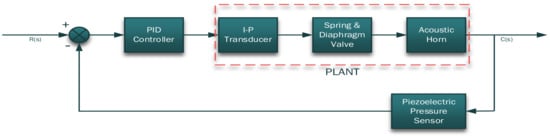
Figure 1. Control system outlook.

In this instance, the plant is considered to be the I-P transducer, spring and diaphragm valve, and ultimately the acoustic horn. The I-P transducer receives a signal in a form of current from the PID controller and translates the current value into pneumatic pressure that activates the spring and diaphragm valve. As the spring and diaphragm valve is driven by the I-P transducer, it consequently actuates the acoustic horn. The acoustic horn operates at the input pneumatic pressure to produce sound waves C(s) that transform into vibrations thereby cleaning the boiler tubes.

It is imperative to note that this is a closed-loop control system. In the feedback path, there is a piezoelectric pressure sensor that monitors the operating pneumatic pressure of the acoustic horn. This is to ensure that the sonic horn is operating at the anticipated pressure. The pressure sensor also serves the purpose of relaying any pressure fluctuations back to the PID controller, and also to alert the user of any excessive pressure in the system that may render the sonic horn to operate above the designed operating pressure.

2.1. Plant

In order to develop a controller, there is a requisite to initially appreciate the plant being controlled [6]. This will aid in designing a compatible controller for the system. The justification for this logic is that the more accurate the plant is modelled, the better the controller will drive the plant [7]. Initially, the plant is considered to be the acoustic horn, since this is what is intended to be controlled and actually drives the process—boiler tube cleaning. It should be noted that the sonic horn is a pneumatic driven component [8]. Therefore, there is a requisite to have subsystems that can convert the PID electronic signals into pneumatic signals. Therefore the plant is a summation of the following subsystems: I-P transducer, spring and diaphragm valve, and the sonic horn.

2.1.1. I-P Transducer

The electrical network circuit of the I-P Transducer comprises a resister R and a capacitor C with a DC supply voltage V(t) and V_o(t) output as illustrated in Figure 2.

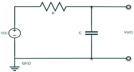
Figure 2. I-P transducer time-domain network circuit.

Assuming zero (0) initial conditions, taking the Laplace transform yields the s-domain circuit as shown in Figure 3.

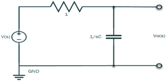
Figure 3. I-P transducer s-domain network circuit.

Nodal analysis at node V_o(s), considering Kirchhoff’s current law yields

$$\frac{{\mathrm{V}}_{\left(\mathrm{s}\right)}-{\mathrm{V}}_{{\mathrm{o}}^{\left(\mathrm{s}\right)}}}{\mathrm{R}}=\frac{{\mathrm{V}}_{{\mathrm{o}}^{\left(\mathrm{s}\right)}}}{\frac{1}{\mathrm{sC}}}$$

(1)

$$\frac{{\mathrm{V}}_{\left(\mathrm{s}\right)}}{\mathrm{R}}{=\mathrm{V}}_{\mathrm{o}\left(\mathrm{s}\right)}\mathrm{sC}+\frac{{\mathrm{V}}_{{\mathrm{o}}^{\left(\mathrm{s}\right)}}}{\mathrm{R}}$$

(2)

$$\frac{{\mathrm{V}}_{\left(\mathrm{s}\right)}}{\mathrm{R}}{=\mathrm{V}}_{{\mathrm{o}}^{\left(\mathrm{s}\right)}}\left(\mathrm{sC}+\frac{1}{\mathrm{R}}\right)$$

(3)

$$\frac{{\mathrm{V}}_{\left(\mathrm{s}\right)}}{\mathrm{R}}{=\mathrm{V}}_{{\mathrm{o}}^{\left(\mathrm{s}\right)}}\left(\frac{\mathrm{sCR}+1}{\mathrm{R}}\right)$$

(4)

$$\frac{{\mathrm{V}}_{{\mathrm{o}}^{\left(\mathrm{s}\right)}}}{{\mathrm{V}}_{\left(\mathrm{s}\right)}}=\frac{\mathrm{R}}{\mathrm{sCR}+1}$$

(5)

$$\therefore \frac{{\mathrm{V}}_{{\mathrm{o}}^{\left(\mathrm{s}\right)}}}{{\mathrm{V}}_{\left(\mathrm{s}\right)}}{=\mathrm{G}}_{1^{\left(\mathrm{s}\right)}}$$

(6)

The I-P transducer is characterized as a continuous-time transfer function labelled ${\mathrm{G}}_{1^{\left(\mathrm{s}\right)}}$.

2.1.2. Spring, Diaphragm Valve, and Acoustic Horn

The spring and diaphragm valve is paired with the acoustic horn to form a mechanical translational system, that is classified as a second degree of freedom (DOF) mass spring damper system depicted in Figure 4 [9]. This approach is justified on the logic that the valve has a direct influence on the sonic horn’s operating pressure.

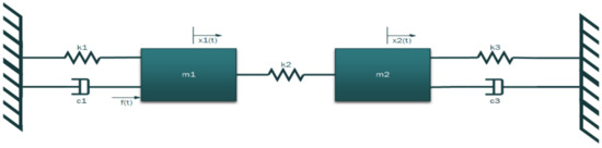
Figure 4. Second DOF mass spring damper system (spring and diaphragm valve and sonic horn).

Table 1 explains what each variable in Figure 4 signifies.

Table 1. Second DOF mass spring damper variables properties.

Variables	Parameter
m1	Valve diaphragm mass
m2	Acoustic horn diaphragm mass
k1	Valve spring constant
k2	Force multiplier
k3	Acoustic horn spring constant
c1	Damping coefficient @m1
c3	Damping coefficient @m2

Isolating mass one (1) as a free body diagram (FBD) as illustrated in Figure 5, all forces exerting on the valve diaphragm are demonstrated.

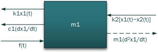
Figure 5. Mass 1 FBD.

Mass one (1) is subject to Newton’s second law of motion:

$$\sum {\mathrm{F}=\mathrm{m}}_1\mathrm{a}$$

(7)

$$+\mathrm{ev}\underrightarrow{{\displaystyle \sum }}{\mathrm{F}=\mathrm{m}}_1\frac{{\mathrm{d}}^2{\mathrm{x}}_1}{{\mathrm{dt}}^2}$$

(8)

$$-{\mathrm{k}}_1{\mathrm{x}}_1-{\mathrm{c}}_1\frac{{\mathrm{dx}}_1}{\mathrm{dt}}-{\mathrm{k}}_2\left({\mathrm{x}}_1-{\mathrm{x}}_2\right){+\mathrm{f}}_{\left(\mathrm{t}\right)}{=\mathrm{m}}_1\frac{{\mathrm{d}}^2{\mathrm{x}}_1}{{\mathrm{dt}}^2}$$

(9)

Assuming zero (0) initial conditions, the Laplace transform of Equation (9) yields Equation (10).

$$-{\mathrm{k}}_1{\mathrm{X}}_{1^{\left(\mathrm{s}\right)}}-{\mathrm{c}}_1{\mathrm{sX}}_{1^{\left(\mathrm{s}\right)}}-{\mathrm{k}}_2\left({\mathrm{X}}_{1^{\left(\mathrm{s}\right)}}-{\mathrm{X}}_{2^{\left(\mathrm{s}\right)}}\right){+\mathrm{F}}_{\left(\mathrm{s}\right)}{=\mathrm{m}}_1{\mathrm{s}}^2{\mathrm{X}}_{1^{\left(\mathrm{s}\right)}}$$

(10)

$${\mathrm{F}}_{\left(\mathrm{s}\right)}{=\mathrm{m}}_1{\mathrm{s}}^2{\mathrm{X}}_{1^{\left(\mathrm{s}\right)}}{+\mathrm{k}}_1{\mathrm{X}}_{1^{\left(\mathrm{s}\right)}}{+\mathrm{c}}_1{\mathrm{sX}}_{1^{\left(\mathrm{s}\right)}}{+\mathrm{k}}_2\left({\mathrm{X}}_{1^{\left(\mathrm{s}\right)}}-{\mathrm{X}}_{2^{\left(\mathrm{s}\right)}}\right)$$

(11)

$${\mathrm{F}}_{\left(\mathrm{s}\right)}{=\mathrm{X}}_{1^{\left(\mathrm{s}\right)}}\left({\mathrm{m}}_1{\mathrm{s}}^2{+\mathrm{c}}_1{\mathrm{s}+\mathrm{k}}_1{+\mathrm{k}}_2\right)-{\mathrm{X}}_{2^{\left(\mathrm{s}\right)}}\left({\mathrm{k}}_2\right)$$

(12)

Mass two (2) is also isolated as a free body diagram (FBD), considering all the forces that are exerting on the acoustic horn’s diaphragm as shown in Figure 6.

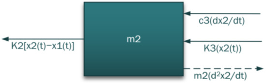
Figure 6. Mass 2 FBD.

Mass two (2) is also subject to Newton’s second law of motion, such that

$$\sum {\mathrm{F}=\mathrm{m}}_2\mathrm{a}$$

(13)

$$+\mathrm{ev}\underrightarrow{{\displaystyle \sum }}{\mathrm{F}=\mathrm{m}}_2\frac{{\mathrm{d}}^2{\mathrm{x}}_2}{{\mathrm{dt}}^2}$$

(14)

$$-{\mathrm{k}}_3{\mathrm{x}}_2-{\mathrm{c}}_3\frac{{\mathrm{dx}}_2}{\mathrm{dt}}-{\mathrm{k}}_2\left({\mathrm{x}}_2{-\mathrm{x}}_1\right){=\mathrm{m}}_2\frac{{\mathrm{d}}^2{\mathrm{x}}_2}{{\mathrm{dt}}^2}$$

(15)

Assuming zero (0) initial conditions, taking the Laplace transform of Equation (15) yields Equation (16).

$$-{\mathrm{k}}_3{\mathrm{X}}_{2^{\left(\mathrm{s}\right)}}-{\mathrm{c}}_3{\mathrm{sX}}_{2^{\left(\mathrm{s}\right)}}-{\mathrm{k}}_2\left({\mathrm{X}}_{2^{\left(\mathrm{s}\right)}}-{\mathrm{X}}_{1^{\left(\mathrm{s}\right)}}\right){=\mathrm{m}}_2{\mathrm{s}}^2{\mathrm{X}}_{2^{\left(\mathrm{s}\right)}}$$

(16)

$${0=\mathrm{m}}_2{\mathrm{s}}^2{\mathrm{X}}_{2^{\left(\mathrm{s}\right)}}{+\mathrm{k}}_1{\mathrm{X}}_{2^{\left(\mathrm{s}\right)}}{+\mathrm{c}}_1{\mathrm{sX}}_{2^{\left(\mathrm{s}\right)}}{+\mathrm{k}}_2\left({\mathrm{X}}_{2^{\left(\mathrm{s}\right)}}-{\mathrm{X}}_{1^{\left(\mathrm{s}\right)}}\right)$$

(17)

$${0=\mathrm{X}}_{2^{\left(\mathrm{s}\right)}}\left({\mathrm{m}}_2{\mathrm{s}}^2{+\mathrm{c}}_3{\mathrm{s}+\mathrm{k}}_3{+\mathrm{k}}_2\right)-{\mathrm{X}}_{1^{\left(\mathrm{s}\right)}}\left({\mathrm{k}}_2\right)$$

(18)

Solving linear Equations (12) and (18) through the matrix method yields Equation (19).

$$\left[\begin{array}{cc}{\mathrm{m}}_1{\mathrm{s}}^2{+\mathrm{c}}_1{\mathrm{s}+\mathrm{k}}_1{+\mathrm{k}}_2& -{\mathrm{k}}_2\\ -{\mathrm{k}}_2& {\mathrm{m}}_2{\mathrm{s}}^2{+\mathrm{c}}_3{\mathrm{s}+\mathrm{k}}_3{+\mathrm{k}}_2\end{array}\right]\left[\begin{array}{c}{\mathrm{X}}_{1^{\left(\mathrm{s}\right)}}\\ {\mathrm{X}}_{2^{\left(\mathrm{s}\right)}}\end{array}\right]=\left[\begin{array}{c}{\mathrm{F}}_{\left(\mathrm{s}\right)}\\ 0\end{array}\right]$$

(19)

Applying Cramer’s rule to Equation (19) yields the following:

$${\mathrm{X}}_{2^{\left(\mathrm{s}\right)}}=\frac{\left|\begin{array}{cc}{\mathrm{m}}_1{\mathrm{s}}^2{+\mathrm{c}}_1{\mathrm{s}+\mathrm{k}}_1{+\mathrm{k}}_2& {\mathrm{F}}_{\left(\mathrm{s}\right)}\\ -{\mathrm{k}}_2& 0\end{array}\right|}{\left|\begin{array}{cc}{\mathrm{m}}_1{\mathrm{s}}^2{+\mathrm{c}}_1{\mathrm{s}+\mathrm{k}}_1{+\mathrm{k}}_2& -{\mathrm{k}}_2\\ {-\mathrm{k}}_2& {\mathrm{m}}_2{\mathrm{s}}^2{+\mathrm{c}}_3{\mathrm{s}+\mathrm{k}}_3{+\mathrm{k}}_2\end{array}\right|}$$

(20)

$${\mathrm{X}}_{2^{\left(\mathrm{s}\right)}}=\frac{{(\mathrm{k}}_2{)\mathrm{F}}_{\left(\mathrm{s}\right)}}{\left({\mathrm{m}}_1{\mathrm{s}}^2{+\mathrm{c}}_1{\mathrm{s}+\mathrm{k}}_1{+\mathrm{k}}_2\right)\left({\mathrm{m}}_2{\mathrm{s}}^2{+\mathrm{c}}_3{\mathrm{s}+\mathrm{k}}_3{+\mathrm{k}}_2\right)-(-{\mathrm{k}}_2\times -{\mathrm{k}}_2)}$$

(21)

$$\frac{{\mathrm{X}}_{2^{\left(\mathrm{s}\right)}}}{{\mathrm{F}}_{\left(\mathrm{s}\right)}}=\frac{{(\mathrm{k}}_2)}{\left({\mathrm{m}}_1{\mathrm{s}}^2{+\mathrm{c}}_1{\mathrm{s}+\mathrm{k}}_1{+\mathrm{k}}_2\right)\left({\mathrm{m}}_2{\mathrm{s}}^2{+\mathrm{c}}_3{\mathrm{s}+\mathrm{k}}_3{+\mathrm{k}}_2\right)-(-{\mathrm{k}}_2\times -{\mathrm{k}}_2)}$$

(22)

$$\therefore \frac{{\mathrm{X}}_{2^{\left(\mathrm{s}\right)}}}{{\mathrm{F}}_{\left(\mathrm{s}\right)}}{=\mathrm{G}}_{{\mathrm{vs}}^{\left(\mathrm{s}\right)}}$$

(23)

Equation (22) can be further be expanded through multiplication. However, the expression would be cumbersome to compute more, especially when assigning physical parameters (which will be demonstrated later). Therefore, this expression will be considered to be the characterized continuous-time transfer function of the actuator valve and acoustic horn subsystems denoted as ${\mathrm{G}}_{{\mathrm{vs}}^{\left(\mathrm{s}\right)}}$.

2.1.3. Piezoelectric Pressure Sensor

The piezoelectric pressure sensor is a mechanical translational system of a single degree of freedom (DOF) type as shown in Figure 7 [10].

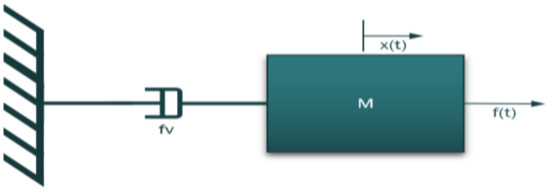
Figure 7. Piezoelectric pressure sensor 1 DOF mass damper system.

A parallel analogous electrical circuit is drawn for the mechanical system in Figure 8, where mass M is converted into a capacitor, and the damper ${\mathrm{f}}_{\mathrm{v}}$ is converted into a resistor.

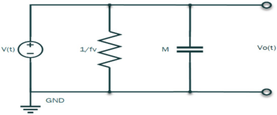
Figure 8. Parallel analogous circuit (time-domain).

Assuming zero (0) initial conditions, taking the Laplace transform of the time-domain circuit yields the s-domain circuit as shown in Figure 9.

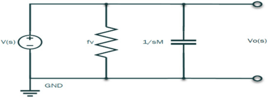
Figure 9. Piezoelectric pressure sensor Laplace transformed parallel analogous circuit.

In view of the transformed network circuit in Figure 9, nodal analysis at node V_o(s) and considering Kirchhoff’s current law yields the following computations:

$${\mathrm{V}}_{\left(\mathrm{s}\right)}=\frac{{\mathrm{V}}_{{\mathrm{o}}^{\left(\mathrm{s}\right)}}}{\frac{1}{\mathrm{sM}}}+\frac{{\mathrm{V}}_{{\mathrm{o}}^{\left(\mathrm{s}\right)}}}{{\mathrm{f}}_{\mathrm{v}}}$$

(24)

$${\mathrm{V}}_{\left(\mathrm{s}\right)}{=\mathrm{V}}_{\mathrm{o}\left(\mathrm{s}\right)}\mathrm{sM}+\frac{{\mathrm{V}}_{{\mathrm{o}}^{\left(\mathrm{s}\right)}}}{{\mathrm{f}}_{\mathrm{v}}}$$

(25)

$${\mathrm{V}}_{\left(\mathrm{s}\right)}{=\mathrm{V}}_{{\mathrm{o}}^{\left(\mathrm{s}\right)}}\left(\mathrm{sM}+\frac{1}{{\mathrm{f}}_{\mathrm{v}}}\right)$$

(26)

$${\mathrm{V}}_{\left(\mathrm{s}\right)}{=\mathrm{V}}_{{\mathrm{o}}^{\left(\mathrm{s}\right)}}\left(\frac{{\mathrm{sMf}}_{\mathrm{v}}+1}{{\mathrm{f}}_{\mathrm{v}}}\right)$$

(27)

$$\frac{{\mathrm{V}}_{{\mathrm{o}}^{\left(\mathrm{s}\right)}}}{{\mathrm{V}}_{\left(\mathrm{s}\right)}}=\frac{{\mathrm{f}}_{\mathrm{v}}}{{\mathrm{sMf}}_{\mathrm{v}}+1}$$

(28)

$$\therefore \frac{{\mathrm{V}}_{{\mathrm{o}}^{\left(\mathrm{s}\right)}}}{{\mathrm{V}}_{\left(\mathrm{s}\right)}}{=\mathrm{H}}_{\left(\mathrm{s}\right)}$$

(29)

The piezoelectric pressure sensor is denoted as a continuous-time transfer function labelled ${\mathrm{H}}_{\left(\mathrm{s}\right)}$.

2.2. Plant Parameter Formulation

Transfer functions of subsystems have been established as continuous-time types. Plant parameters will be estimated taking into consideration realistic modelling, readily available information, and reasonable assumptions where applicable.

2.2.1. Electrical Systems

The I-P transducer circuit comprises of a resistor and a capacitor as shown previously in Figure 2. The resistor and capacitor values are assumed to be 1 Ω and 1 F, respectively. Similarly, the piezoelectric pressure sensor analogous circuit components M and ${\mathrm{f}}_{\mathrm{v}}$ are assumed to be 0.01 F and 1 Ω, respectively.

2.2.2. Mechanical Translational Systems

The masses in concern are the diaphragms of the spring and diaphragm valve and the acoustic horn as illustrated in Figure 10 and Figure 11, respectively.

Figure 10. Silicon nitride diaphragm.

Figure 11. Titanium diaphragm.

Assigning input characteristics into the valve’s diaphragm 3D model, as shown in Table 2, yields the summarized results from the Autodesk^® Inventor^® software as shown in Table 3.

Table 2. Silicon nitride diaphragm input parameters [11].

Parameter	Value
Material	Silicon Nitride
Thickness (mm)	30
Diameter (mm)	297
Requested accuracy level	Very high

Table 3. Physical properties of a silicon nitride diaphragm.

General Properties	Value
Material	Silicon Nitride
Density	3.180 g/cm3
Mass	6.609 kg (Relative Error = 0.000000%)
Area	166,549.964 mm2 (Relative Error = 0.000000%)
Volume	2,078,375.598 mm3 (Relative Error = 0.000000%)

Assigning input characteristics into the acoustic horn’s diaphragm 3D model, as shown in Table 4, yields summarized results from the Autodesk^® Inventor^® software as shown in Table 5.

Table 4. Titanium diaphragm input parameters [12].

Parameter	Value
Material	Titanium
Thickness (mm)	1
Diameter (mm)	367
Requested accuracy level	Very high

Table 5. Physical properties of a titanium diaphragm.

General Properties	Value
Material	Titanium
Density	4.510 g/cm3
Mass	0.477 kg (Relative Error = 0.000000%)
Area	212,721.951 mm2 (Relative Error = 0.000000%)
Volume	105,784.493 mm3 (Relative Error = 0.000000%)

Considering the extracted information for the diaphragms, mass values ${\mathrm{m}}_1$ and ${\mathrm{m}}_2$ in relation to the second degree of freedom mass spring damper system in Figure 4 are 0.477 and 6.609 kg, respectively. Table 6 shows the input parameters required to design the acoustic horn’s spring model using the Autodesk^® Inventor^® Professional Design Accelerator software.

Table 6. Acoustic horn spring constant input parameters.

Design Inputs
Installed length type		Custom
Coil length (mm)		40
Coil direction		Right Direction
Spring start	Closed end coils (µL)	1.5
	Transition coils (µL)	1
	Ground coils (µL)	0.75
Spring end	Closed end coils (µL)	1
	Transition coils (µL)	0.75
	Ground coils (µL)	0.5
Calculation Inputs
Minimum load length (mm)		45
Maximum load length (mm)		39.270
Working stroke (mm)		5.730
Spring material predetermined values	Ultimate tensile stress (MPa)	1860
	Allowable torsional stress (MPa)	930
	Modulus of elasticity in shear (MPa)	68,500
	Density (kg/m3)	7850
	Utilization factor of material (µL)	0.9

The design accelerator spring environment deemed the spring with the properties in Table 7 as compliant. Therefore, the spring constant to be considered for ${\mathrm{k}}_3$ is 175 N/m. Spring constant ${\mathrm{k}}_2$ is assumed to be 1 N/m. Spring constant ${\mathrm{k}}_1$ can be computed from Hook’s law with formula,

$${\mathrm{F}=\mathrm{k}}_1\mathrm{u}$$

(30)

where

$$\mathrm{F}=10.23 \mathrm{N}, \mathrm{u}=19 \mathrm{mm}$$

Table 7. Acoustic horn’s spring properties.

General Properties	Value
$\mathrm{Space} \mathrm{between} \mathrm{coils} \mathrm{of} \mathrm{free} \mathrm{spring} (\mathsf{\alpha }$)	3.172 mm
$\mathrm{Pitch} \mathrm{of} \mathrm{free} \mathrm{spring} (\mathrm{t}$)	3802 mm
$\mathrm{Stress} \mathrm{concentration} \mathrm{factor} ({\mathrm{K}}_{\mathrm{w}}$)	1 µL
$\mathrm{Spring} \mathrm{constant} (\mathrm{k}$)	0.175 N/mm
$\mathrm{Minimum} \mathrm{load} \mathrm{spring} \mathrm{deflection} ({\mathrm{s}}_1$)	29,649 mm
$\mathrm{Total} \mathrm{spring} \mathrm{deflection} ({\mathrm{s}}_8$)	34,379 mm
$\mathrm{Limit} \mathrm{spring} \mathrm{deflection} ({\mathrm{s}}_9$)	60,262 mm
$\mathrm{Limit} \mathrm{test} \mathrm{length} \mathrm{of} \mathrm{spring} ({\mathrm{L}}_{\mathrm{minf}}$)	16,872 mm
$\mathrm{Theoretic} \mathrm{limit} \mathrm{length} \mathrm{of} \mathrm{spring} ({\mathrm{L}}_9$)	13,388 mm
$\mathrm{Spring} \mathrm{limit} \mathrm{force} ({\mathrm{F}}_9$)	10,517 N
$\mathrm{Minimum} \mathrm{load} \mathrm{stress} ({\mathsf{\tau }}_1$)	377,287 MPa
$\mathrm{Maximum} \mathrm{load} \mathrm{stress} ({\mathsf{\tau }}_8$)	452,744 MPa
$\mathrm{Solid} \mathrm{length} \mathrm{stress} ({\mathsf{\tau }}_9$)	793,600 MPa
$\mathrm{Critical} \mathrm{speed} \mathrm{of} \mathrm{spring} (\mathrm{v}$)	10,394 mps
$\mathrm{Natural} \mathrm{frequency} \mathrm{of} \mathrm{spring} \mathrm{surge} (\mathrm{f}$)	200,787 Hz
$\mathrm{Deformation} \mathrm{energy} ({\mathrm{W}}_8$)	0.103 J
$\mathrm{Wire} \mathrm{length} (\mathrm{l}$)	509,767 mm
$\mathrm{Spring} \mathrm{mass} (\mathrm{m}$)	0.001 kg

$\mathrm{F}$ and $\mathrm{u}$ are the maximum allowable thrust and travel, respectively. These parameters are referenced from a readily available property table of spring and diaphragm valve suitable for this operation [11]. Substituting $\mathrm{F}$ and $\mathrm{u}$ into Equation (30) yields

$$10{.23=\mathrm{k}}_1{19\times 10}^{-3}$$

(31)

$${\mathrm{k}}_1=538.473 \mathrm{N}/\mathrm{m}$$

(32)

Damping coefficients ${\mathrm{c}}_1$ and ${\mathrm{c}}_3$ are determined mathematically now that ${\mathrm{m}}_1$, ${\mathrm{m}}_2$, ${\mathrm{k}}_1$, and ${\mathrm{k}}_3$ are known. Both subsystems are assigned steel damping properties of 1% overshoot ratio [13]. Considering the % overshoot formula,

$${\%\mathrm{OS}=\mathrm{e}}^{-(\mathsf{\zeta }\mathsf{\pi }/\sqrt{1-{\mathsf{\zeta }}^2})}\times 100$$

(33)

The inverse of Equation (33) yields the formula to compute the damping ratio $\mathsf{\zeta }$:

$$\mathsf{\zeta }=\frac{-\ln (\%\mathrm{OS}/100)}{\sqrt{{\mathsf{\pi }}^2{+\ln }^2(\%\mathrm{OS}/100)}}$$

(34)

$$\mathsf{\zeta }=\frac{-\ln (1/100)}{\sqrt{{\mathsf{\pi }}^2{+\ln }^2(1/100)}}$$

(35)

$$\mathsf{\zeta }=0.826$$

(36)

Expression (36) suggests that both systems are underdamped due to the damping ratio being less than 1 [14]. The natural frequency of the spring and diaphragm valve is calculated as

$${\mathsf{\omega }}_{\mathrm{n}1}=\sqrt{\frac{{\mathrm{k}}_1}{{\mathrm{m}}_1}}$$

(37)

$${\mathsf{\omega }}_{\mathrm{n}1}=\sqrt{\frac{538.473}{6.609}}$$

(38)

$${\mathsf{\omega }}_{\mathrm{n}1}=9.026 \mathrm{rad}/\mathrm{s}$$

(39)

With critical damping coefficient

$${\mathrm{C}}_{\mathrm{c}1}{=2\mathrm{m}}_1{\mathsf{\omega }}_{\mathrm{n}1}$$

(40)

$${\mathrm{C}}_{\mathrm{c}1}=2(6.609\left)\right(9.026)$$

(41)

$${\mathrm{C}}_{\mathrm{c}1}=119.305 \mathrm{Ns}/\mathrm{m}$$

(42)

Therefore, damping coefficient ${\mathrm{c}}_1$ is

$$\mathsf{\zeta }=\frac{{\mathrm{c}}_1}{{\mathrm{C}}_{\mathrm{c}1}}$$

(43)

$${\mathrm{c}}_1=(0.826\left)\right(119.305)$$

(44)

$${\mathrm{c}}_1=98.546 \mathrm{Ns}/\mathrm{m}$$

(45)

The natural frequency of the acoustic horn is calculated as follows:

$${\mathsf{\omega }}_{\mathrm{n}2}=\sqrt{\frac{{\mathrm{k}}_3}{{\mathrm{m}}_2}}$$

(46)

$${\mathsf{\omega }}_{\mathrm{n}2}=\sqrt{\frac{175}{0.477}}$$

(47)

$${\mathsf{\omega }}_{\mathrm{n}2}=19.154 \mathrm{rad}/\mathrm{s}$$

(48)

With critical damping coefficient

$${\mathrm{C}}_{\mathrm{c}2}{=2\mathrm{m}}_2{\mathsf{\omega }}_{\mathrm{n}2}$$

(49)

$${\mathrm{C}}_{\mathrm{c}2}=2(0.477\left)\right(19.154)$$

(50)

$${\mathrm{C}}_{\mathrm{c}2}=18.273 \mathrm{Ns}/\mathrm{m}$$

(51)

Therefore, damping coefficient ${\mathrm{c}}_3$ is

$$\mathsf{\zeta }=\frac{{\mathrm{c}}_3}{{\mathrm{C}}_{\mathrm{c}2}}$$

(52)

$${\mathrm{c}}_3=(0.826\left)\right(18.273)$$

(53)

$${\mathrm{c}}_3=15.093 \mathrm{Ns}/\mathrm{m}$$

(54)

Table 8 shows a summary of the estimated physical properties of the subsystems in concern. For computation purposes and defining final representations of transfer functions, the values are rounded off to two decimal points where applicable.

Table 8. Multiple subsystem parameters summary.

Electrical Systems
$\mathrm{R}$	1 Ω
$\mathrm{C}$	1 F
$\mathrm{M}$	0.01 Ω
${\mathrm{f}}_{\mathrm{v}}$	1 Ns/m
Mechanical Systems
${\mathrm{m}}_1$	6.61 kg
${\mathrm{m}}_2$	0.48 kg
${\mathrm{k}}_1$	538.47 N/m
${\mathrm{k}}_2$	1 N/m
${\mathrm{k}}_3$	175 N/m
${\mathrm{c}}_1$	98.55 Ns/m
${\mathrm{c}}_3$	15.09 Ns/m

2.2.3. Subsystems’ Final Transfer Function Representations

The I-P transducer with transfer function ${\mathrm{G}}_{1^{\left(\mathrm{s}\right)}}$:

$${\mathrm{G}}_{1^{\left(\mathrm{s}\right)}}=\frac{{\mathrm{V}}_{{\mathrm{o}}^{\left(\mathrm{s}\right)}}}{{\mathrm{V}}_{\left(\mathrm{s}\right)}}=\frac{\mathrm{R}}{\mathrm{sCR}+1}$$

(55)

where

$$\mathrm{R}=1 \mathsf{\Omega }, \mathrm{C}=1 \mathrm{F}$$

From Equation (6), the final transfer function is:

$${\mathrm{G}}_{1^{\left(\mathrm{s}\right)}}=\frac{{\mathrm{V}}_{{\mathrm{o}}^{\left(\mathrm{s}\right)}}}{{\mathrm{V}}_{\left(\mathrm{s}\right)}}=\frac{1}{\mathrm{s}\left(1\right)\left(1\right)+1}$$

(56)

$${\mathrm{G}}_{1^{\left(\mathrm{s}\right)}}=\frac{{\mathrm{V}}_{{\mathrm{o}}^{\left(\mathrm{s}\right)}}}{{\mathrm{V}}_{\left(\mathrm{s}\right)}}=\frac{1}{\mathrm{s}+1}$$

(57)

It is imperative to note that the spring and diaphragm valve and the acoustic horn were modelled as a second degree of freedom mass spring damper system with transfer function ${\mathrm{G}}_{{\mathrm{va}}^{\left(\mathrm{s}\right)}}$. For the purpose of assigning the estimated physical properties, the spring and diaphragm valve and the acoustic horn are considered as separate entities from an equation point of view, with new equations ${\mathrm{G}}_{2^{\left(\mathrm{s}\right)}}$ and ${\mathrm{G}}_{3^{\left(\mathrm{s}\right)}}$, respectively. This is the inverse phenomenon of the convolution theorem of two functions, in this case equation ${\mathrm{G}}_{2^{\left(\mathrm{s}\right)}}$ and ${\mathrm{G}}_{3^{\left(\mathrm{s}\right)}}$, which yield the same step response as with equation ${\mathrm{G}}_{{\mathrm{va}}^{\left(\mathrm{s}\right)}}$ [15]. Considering the spring and diaphragm valve transfer function ${\mathrm{G}}_{2^{\left(\mathrm{s}\right)}}$:

$${\mathrm{G}}_{2^{\left(\mathrm{s}\right)}}=\frac{{\mathrm{X}}_{2^{\left(\mathrm{s}\right)}}}{{\mathrm{F}}_{\left(\mathrm{s}\right)}}=\frac{{\mathrm{k}}_2}{{\mathrm{m}}_1{\mathrm{s}}^2{+\mathrm{c}}_1{\mathrm{s}+\mathrm{k}}_1}$$

(58)

where

$${\mathrm{m}}_1=6{.61 \mathrm{kg}; \mathrm{c}}_1=98{.55 \mathrm{Ns}/\mathrm{m}; \mathrm{k}}_1=538.47 \mathrm{N}/\mathrm{m}$$

From Equation (58), the final transfer function is:

$${\mathrm{G}}_{2^{\left(\mathrm{s}\right)}}=\frac{{\mathrm{X}}_{2^{\left(\mathrm{s}\right)}}}{{\mathrm{F}}_{\left(\mathrm{s}\right)}}=\frac{1}{\left(6.61\right){\mathrm{s}}^2+\left(98.55\right)\mathrm{s}+538.47}$$

(59)

$${\mathrm{G}}_{2^{\left(\mathrm{s}\right)}}=\frac{{\mathrm{X}}_{2^{\left(\mathrm{s}\right)}}}{{\mathrm{F}}_{\left(\mathrm{s}\right)}}=\frac{1}{6{.61\mathrm{s}}^2+98.55\mathrm{s}+538.47}$$

(60)

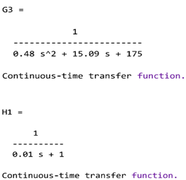
Acoustic horn with transfer function ${\mathrm{G}}_{3^{\left(\mathrm{s}\right)}}$:

$${\mathrm{G}}_{3^{\left(\mathrm{s}\right)}}=\frac{{\mathrm{X}}_{2^{\left(\mathrm{s}\right)}}}{{\mathrm{F}}_{\left(\mathrm{s}\right)}}=\frac{{\mathrm{k}}_2}{{\mathrm{m}}_2{\mathrm{s}}^2{+\mathrm{c}}_3{\mathrm{s}+\mathrm{k}}_3}$$

(61)

where

$${\mathrm{m}}_2=0{.48 \mathrm{kg}; \mathrm{c}}_3=15{.09 \mathrm{Ns}/\mathrm{m}; \mathrm{k}}_3=175 \mathrm{N}/\mathrm{m}$$

From Equation (61), the final transfer function is:

$${\mathrm{G}}_{3^{\left(\mathrm{s}\right)}}=\frac{{\mathrm{X}}_{2^{\left(\mathrm{s}\right)}}}{{\mathrm{F}}_{\left(\mathrm{s}\right)}}=\frac{1}{(0{.48)\mathrm{s}}^2+\left(15.09\right)\mathrm{s}+175}$$

(62)

$${\mathrm{G}}_{3^{\left(\mathrm{s}\right)}}=\frac{{\mathrm{X}}_{2^{\left(\mathrm{s}\right)}}}{{\mathrm{F}}_{\left(\mathrm{s}\right)}}=\frac{1}{0{.48\mathrm{s}}^2+15.09\mathrm{s}+175}$$

(63)

Considering the piezoelectric pressure sensor with transfer function ${\mathrm{H}}_{\left(\mathrm{s}\right)}$:

$${\mathrm{H}}_{\left(\mathrm{s}\right)}=\frac{{\mathrm{V}}_{{\mathrm{o}}^{\left(\mathrm{s}\right)}}}{{\mathrm{V}}_{\left(\mathrm{s}\right)}}=\frac{{\mathrm{f}}_{\mathrm{v}}}{{\mathrm{sMf}}_{\mathrm{v}}+1}$$

(64)

where

$$\mathrm{M}=0{.01 \mathrm{kg}; \mathrm{f}}_{\mathrm{v}}=1 \mathrm{Ns}/\mathrm{m}$$

From Equation (64), the final transfer function is represented as follows:

$${\mathrm{H}}_{\left(\mathrm{s}\right)}=\frac{{\mathrm{V}}_{{\mathrm{o}}^{\left(\mathrm{s}\right)}}}{{\mathrm{V}}_{\left(\mathrm{s}\right)}}=\frac{1}{\mathrm{s}(0.01\left)\right(1)+1}$$

(65)

$${\mathrm{H}}_{\left(\mathrm{s}\right)}=\frac{{\mathrm{V}}_{{\mathrm{o}}^{\left(\mathrm{s}\right)}}}{{\mathrm{V}}_{\left(\mathrm{s}\right)}}=\frac{1}{0.01\mathrm{s}+1}$$

(66)

2.3. Multiple Subsystem Reduction

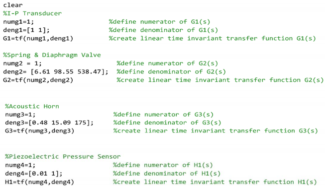
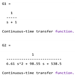
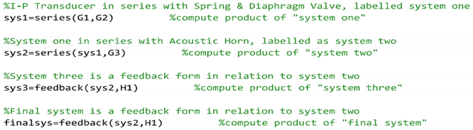
The system configuration previously illustrated in Figure 1 has been redrawn in a cascaded form as shown in Figure 12 [16]. The subsystem blocks are now labelled according to their modelled transfer functions. A single transfer function representation for this interconnecting system is derived herein through a cascaded form topology to reduce the system into a single block for further analysis [17]. Creating linear time invariant transfer function scripts of the controlled plant in MATLAB^®:

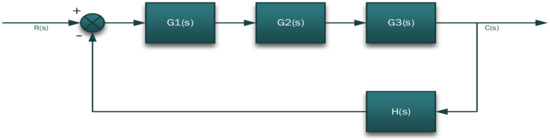
Figure 12. System block diagram.

Script output:

Multiple subsystem reduction script:

Script output:

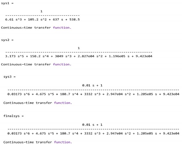
${\mathrm{Final}}_{\mathrm{sys}}$ is the equivalent transfer function of the control system, which is also represented in a block form as illustrated in Figure 13.

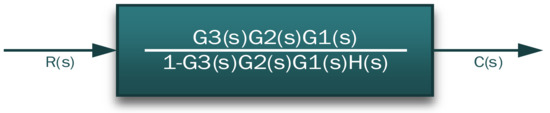
Figure 13. Equivalent control system transfer function Final_sys.

2.4. PID Controller

Figure 14 illustrates the updated system configuration that comprises a step function input, summing block, PID controller, reduced plant block-Final_sys, graphical scope display, numeric output display, set pace, and signal lines.

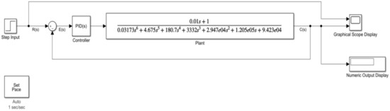
Figure 14. Closed-loop system configuration.

2.4.1. Design Requirements

In order to derive design requirements of the controller, the controlled variable is analysed based on the operating conditions. The sonic horn is required to dislodge soot particles from the tubes immediately when activated. This immediate activation produces sudden sound waves which will induce vibration that will dislodge ash agglomeration [18]. From this scenario, it is deduced that there is a requirement of an instantaneous full capacity pneumatic pressure application. This immediate activation requirement will translate into an instantaneous rise time from a control point of view [19].

A second factor to consider is the desired sound frequency to clean and maintain allowable vibrations that will not damage the boiler substructure components. The already developed acoustic horn’s operating condition is specified to function at a pneumatic pressure of 552 kPa in order to propagate a sound frequency of 75 Hz [20]. This suggests that any value above or below this frequency has a potential to damage the boiler’s internal components, annoy plant personnel, and be inefficient at removing soot particles. Based on this constraint, the controller is required to maintain and not exceed the specified frequency continuum. This requirement translates to acceptable minimal % overshoot or no % overshoot if possible.

The steady-state error and stability are required to be quickly attained. These factors govern the ability of the acoustic horn to maintain the operating pneumatic pressure and sound frequency to permit the cleaning of the boiler tubes [21]. As a safety factor, a scenario of supply pneumatic pressure fluctuations into the system is taken into consideration, where the controller needs to reject these disturbances. These disturbance scenarios into the system will be demonstrated later in Section 3.4 under simulation environments. Table 9 gives a summarized outlook for the controller requirements to be incorporated into the design process.

Table 9. Controller design requirements.

Parameter	Value
$\mathrm{Rise} \mathrm{time} ({\mathrm{T}}_{\mathrm{r}}$)	0.5 s
$\mathrm{Settling} \mathrm{time} ({\mathrm{T}}_{\mathrm{s}}$)	1.5 s
% Overshoot	0–0.9%
Closed-loop stability	Stable
Aggressive/Robust	Robust

Table 10 gives hypothesized plant behaviour when subjected to an input.

Table 10. Control system operating requirements.

Parameter	Value
$\mathrm{Rise} \mathrm{time} ({\mathrm{T}}_{\mathrm{r}}$)	0.5 s
$\mathrm{Settling} \mathrm{time} ({\mathrm{T}}_{\mathrm{s}}$)	1.5 s
% Overshoot	0–0.9
Closed-loop stability	Stable

2.4.2. PID Design

A step function plot script of the equivalent transfer function ${\mathrm{Final}}_{\mathrm{sys}}$ is as follows: A step response plot of system ${\mathrm{Final}}_{\mathrm{sys}}$ as illustrated in Figure 15 suggests that the system does not meet the design requirements. Although the step response plot is as anticipated, the system has a rise time of 2.22 s, a settling time of 4.19 s, and a final value of 1.06 × 10⁻⁵. Comparing these results with Table 10 suggests that designing a controller is the next necessary step to achieve the design requirements.

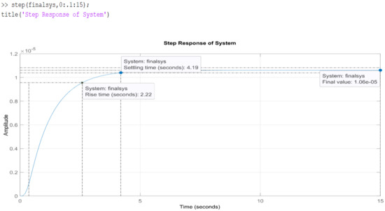
Figure 15. Final_sys step response.

The PID controller block is expanded in view as shown in Figure 16. The proportional (K_p), integrative (K_i), and derivative (K_d) gains are deliberately set to 1. This is undertaken to analyse the system’s response when the controller executes these gains relative to the input command from signal R(s).

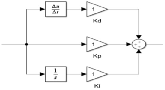
Figure 16. PID controller block expanded view [22].

As observed in Figure 17, when a step input with a 1 s step time, 0 initial value and sampling, and a final value of 1, the system C(s) does not respond to the reference signal R(s).

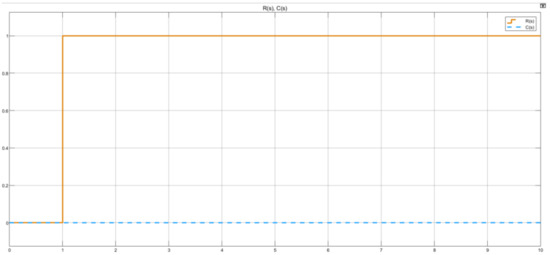
Figure 17. Untuned system reference tracking plot.

The plot in Figure 17 does show that the error is not reduced from a plot point of view. However, it does not give a clear indication of the system’s behaviour from a numeric perspective. The numeric output display indicates the final value of the system to be 9.266 × 10⁻⁵ at 10 s as shown in the system configuration in Figure 18. Relative to the input command of 1, this suggests that the design requirements are still not met.

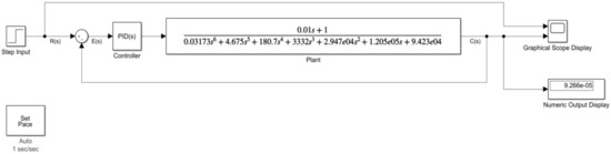
Figure 18. Untuned system output demonstration.

Signal C(s) is isolated and inspected to comprehend the system’s behaviour. Even though the response is infinitesimally diminutive as noted in Figure 17, the system does respond to the input command of a step input. This is concluded by the graph plot in Figure 19, such that after 1 s, the system responds from 0 to 1 × 10⁻⁵ value, thereafter exponentially ramps up to infinity. At this point, the transient response, steady-state error, and stability design objectives are not met.

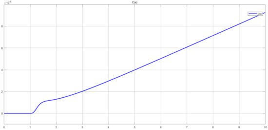
Figure 19. Untuned system C(s) signal.

The controller type of this system is a PID that requires tuning of the gains; K_p, K_i, and K_d in order to satisfy the design objectives.

2.4.3. PID Tuning

PID tuning input parameters are specified in Table 11 as follows.

Table 11. PID tuning settings.

Parameter	Value
Controller	PID
Time domain	Continuous-time
Form	Parallel
Source	Internal
Tuning method	Transfer function based
Zero-crossing detection	Enabled
Compensator formula	$\mathrm{P}+\mathrm{I}\frac{1}{\mathrm{s}}+\mathrm{D}\frac{\mathrm{N}}{1+\mathrm{N}\frac{1}{\mathrm{s}}}$

Considering the tuning settings and the compensator formula, P is the proportional gain, D is the derivative gain, I is the integrative gain, and N is the filter coefficient. The plant is linearized, and an improved control system step response is deduced in Figure 20. A reference tracking focused approach is adopted to tune the controller gains. The tuned response plot in Figure 20 shows some significant system improvements such that the final value is 1, as per input step function command. Furthermore, the system now has a rise time of 0.752 s and a settling time of 3.13 s.

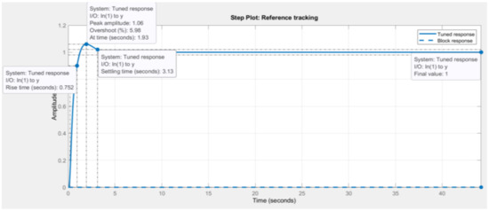
Figure 20. Tuned system response (reference tracking focus).

Table 12 and Table 13 show a comparison between the untuned system against the tuned system. The newly tuned gains imply that the controller will have a gain margin of 15.7 dB @ 10.3 rad/s and a phase margin of 69 degrees @ 1.81 rad/s. When compared to the untuned gain and phase margins, it is notable that the tuned system has less chances of being unstable. However, with this improved control system there is a 5.98% overshoot peak amplitude 1.06 at 1.93 s incurred.

Table 12. Tuned controller parameters.

Parameter	Tuned	Block
P	183,706.2513	1
I	232,966.3411	1
D	30,144.1142	1
N	206.9837	100

Table 13. Tuned system performance and robustness.

Parameter	Tuned	Block
Rise time	0.752 s	2.07 × 105 s
Settling time	3.13 s	3.69 × 105 s
Overshoot	5.98%	0%
Peak	1.06	1
Gain margin	15.7 dB @ 10.3 rad/s	109 dB @ 12.4 rad/s
Phase margin	69 deg @ 1.81 rad/s	90 deg @ 1.06 × 10−5 rad/s
Compensator formula	Stable	Stable

The amount of % overshoot induced into the system is undesirable as this would mean that the operating sound frequency of the acoustic horn will be much lower than the specified range. As a result, the system further requires to be fine-tuned, for reasons that the rise and settling times as well as the % overshoot still do not meet the design’s initial requirements.

Fine-tuning the controller to be faster by decreasing the response time from 1.104 s to 0.921 s, and adjusting the transient behaviour of the system to be more robust from values 0.69 to 0.6, yields an improved system’s response as shown in Figure 21. The fine-tuned system’s response shows a desirable outcome, such that the final value is still 1, as per input step command, with an improved rise time of 0.562 s, a 0.201% overshoot peak amplitude 1 at 1.05 s, and a settling time of 1.05 s.

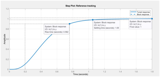
Figure 21. Fine-tuned system response.

Table 14 and Table 15 show the updated controller parameters, performance, and robustness of the control system which have been applied onto the PID controller block. These updated gains K_p = 225,775.49, K_i = 208,064.1457, K_d = 21,780.4129, and N = 248.1711 satisfy the design requirements. It is also vital to note that the closed-loop stability is deemed stable at these newly defined gains.

Table 14. Fine-tuned controller parameters.

Parameter	Tuned	Block
P	225,775.49	225,775.49
I	208,064.1457	208,064.1457
D	21,780.4129	21,780.4129
N	248.1711	248.1711

Table 15. Fine-tuned system performance and robustness.

Parameter	Tuned	Block
Rise time	0.562 s	0.562 s
Settling time	1.05 s	1.05 s
Overshoot	0.201%	0.201%
Peak	1	1
Gain margin	14.2 dB @ 8.81 rad/s	14.2 dB @ 8.81 rad/s
Phase margin	69 deg @ 2.17 rad/s	69 deg @ 2.17 rad/s
Compensator formula	Stable	Stable

From a frequency response perspective, the gain and phase margins are 14.2 dB @ 8.81 rad/s and 69 degrees @ 2.17 rad/s as observed in Table 15. Figure 22 shows the final gains of the PID controller block. Table 16 shows a summary of results compared to design requirements. With these fine-tuned gains, testing of the control system is explored to deduce how it handles various inputs other than a step function.

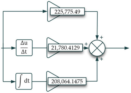
Figure 22. Tuned PID block expanded view.

Table 16. Design summary of results.

Parameter	Requirement	Actual Controller Design	Actual Control System Design
$\mathrm{Rise} \mathrm{time} ({\mathrm{T}}_{\mathrm{r}}$)	0.6 s	0.562 s	0.562 s
$\mathrm{Settling} \mathrm{time} ({\mathrm{T}}_{\mathrm{s}}$)	1.5 s	1.05 s	1.05 s
% Overshoot	0–0.9%	0.201%	0.201%
Closed-loop stability	Stable	Stable	Stable
Aggressive/Robust	Robust (0.69)	Robust (0.6)	Robust (0.6)

3. Testing

In order to test the designed controller, a testing environment was deployed to examine the system’s response when it was subjected to different sources other than a step input. Sources considered were a step input, sinusoidal wave, ramp, and a constant. It is important to be cognizant that the sinusoidal wave and ramp inputs do not permit a settling time scenario based on the nature of their functionality. However, they were only deployed to assess the control system’s reference tracking capabilities. For a step input source, with parameters 1 s step time, 0 initial value, final value of 1, and a sampling time of 0 s, the system responds as anticipated, such that signal C(s) tracks signal R(s) and stabilizes in under 3 s as shown in Figure 23.

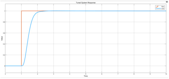
Figure 23. Step input source test graph plot.

For a sinusoidal wave source, with an amplitude of 5 and a frequency of 1 rad/s, in Figure 24, signal C(s) is observed to accurately track signal R(s) over time, such that the system’s amplitudes are approximately ±5 at different planes. The reason for the approximation is that the sine wave source is an alternating wave that does not allow for a settling time as with the step input source. Therefore, this testing scenario only enables an understanding that the system tracks the reference signal as designed.

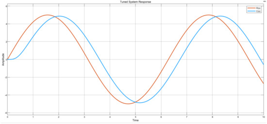
Figure 24. Sine wave source graph plot.

A system with ramp input source properties of 5-degree slope, 0 start time and initial output, at a constant value of 50 yields a system response shown in Figure 25. Signal C(s) responds as the intended ramp input signal R(s). As with the sine wave source, the ramp source also does not facilitate settling time conditions: therefore, this particular test is performed to observe the reference tracking capabilities of the control system.

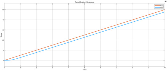
Figure 25. Ramp source graph plot.

Finally, for a constant input source, with an infinity sample time and a constant value of 50, the control system responds and tracks the set point R(s) as seen in Figure 26, whereby also signal C(s) is observed to behave as designed, such that the settling time and stability are achieved in under 3 s.

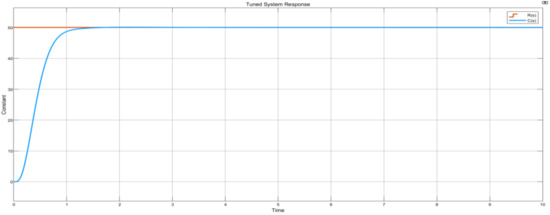
Figure 26. Constant source graph plot.

These testing conditions have illustrated that the designed controller gains are suitable to drive plant (denoted as Final_sys). The requirements met included a quick transient response, system stability, robustness, and accurate reference tracking.

3.1. Simulation of Control System

Based on the satisfied design criteria, controller tuning and testing, simulation of the control system was conducted. The sonic horn is the ultimate driven plant, which operates via pneumatic pressure to produce the desired cleaning sound frequency. Therefore, the simulation environment considers driving the acoustic horn through controlling the pneumatic pressure since this determines the sound frequency.

Simulation was conducted on seven (7) scenarios, with the first four (4) scenarios illustrated in Table 17. These were conducted to observe the behaviour of the control system when the inputs were changed under a continuous simulation. Thereafter, the remaining three (3) scenarios feature a constant input, normal disturbance, and severe disturbance rejection capabilities.

Table 17. Input pressure scenarios.

Set-Point	Pressure
Off	0 kPa
Low	350 kPa
Mid	750 kPa
High	1000 kPa

In relation to the constant input source, this type of simulation was critical as this will be the operating condition that the sonic horn requires to clean the boiler tubes; a steady pressure supply is required. Finally, a disturbance correction environment was conducted to assess how quickly the controller rejects disturbances in order to drive the acoustic horn at the designated pressure supply.

3.2. Varied Set Points Simulation

Figure 27 shows that when the input pressure is set to 0 kPa, the output pressure gauge and the numeric output display also measure 0 kPa.

Figure 27. Input pressure simulation—0 kPa.

When the input pressure is set to low, that is 350 kPa, the output pressure gauge and the numeric output display also measure 350 kPa as illustrated in Figure 28.

Figure 28. Input pressure simulation—350 kPa.

Figure 29 shows the outcome of the system when the input pressure is set to mid, that is 750 kPa, such that the output pressure gauge and the numeric output display read 750 kPa.

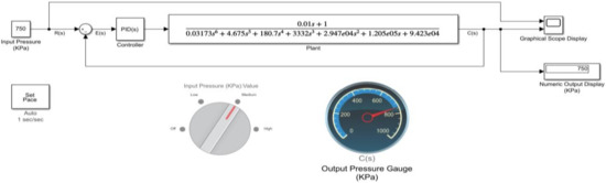
Figure 29. Input pressure simulation—750 kPa.

Finally, when the input pressure is set to high, that is 1000 kPa, the output pressure gauge and the numeric output display also measure 1000 kPa as shown in Figure 30.

Figure 30. Input pressure simulation—1000 kPa.

The control system’s response to the varied set points can be observed in a graphical form in Figure 31. The simulation ran for 90 s with inputs varied at random time intervals. As the pressure inputs were varied, the control system responded to these different commands as designed. This behaviour compares exactly to the anticipated control system response. Another important factor to analyse is that signal C(s) accurately tracks signal R(s).

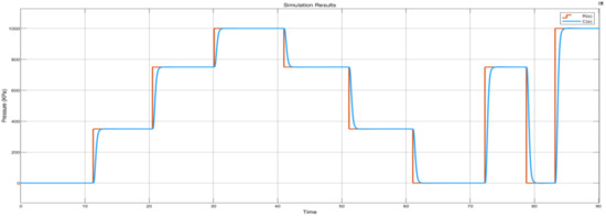
Figure 31. Varied set points continuous simulation results plot.

3.3. Constant Set Point Simulation

The constant set point simulation considers the already specified acoustic horn operating conditions. The design conclusion was that the sonic horn should operate at a pressure of 552 kPa. This established pressure consequently produced a sound frequency of 75 Hz which is suitable for cleaning the boiler tubes while also not inducing damage in the boiler internal components.

Therefore, this particular simulation considers the given pressure set point of 552 kPa, assuming that the required cleaning cycle of the boiler tubes should be 90 s, the simulation was conducted under the presumed cycle time. In the configuration, as shown in Figure 32, the medium setting input transducer has been adjusted to reflect a pressure of 552 kPa.

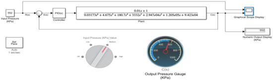
Figure 32. Input pressure simulation—552 kPa.

The graphical results in Figure 33 illustrate that the control system has no unwanted overshoots and that the steady-state error is reached in under 3 s. Furthermore, the system proves to be stable in the simulated operating cycle time.

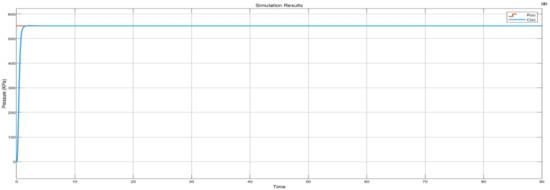
Figure 33. Constant set point simulation results plot.

3.4. Disturbance Rejection Simulation

A disturbance in a sinusoidal time-based wave form was introduced into the control system as shown in Figure 34. The disturbance block was used to simulate pneumatic supply pressure instabilities that may affect the system’s output in relation to the reference signal. The assigned sine wave properties were an amplitude value of 50, a frequency of 1 rad/s, and a sample time of 3 s. The disturbance can be conveyed as a situation where there are pressure supply fluctuations in the pneumatic line as a result of a faulty valve or blockage in the filtration subsystem(s). As the plant is driven at a constant set point of 552 kPa, disturbances were induced into the control system every 10 s. It is observed in Figure 35 that the controller rejects these disturbances in under 2 s to retain the system according to the desired set point.

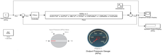
Figure 34. Disturbance correction configured system.

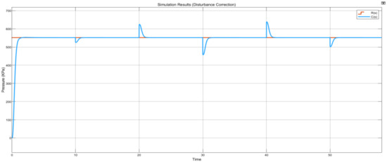
Figure 35. Normal disturbance plot.

Similarly, in a severe disturbances case, the controller corrects these fluctuations in under 2 s as illustrated in Figure 36.

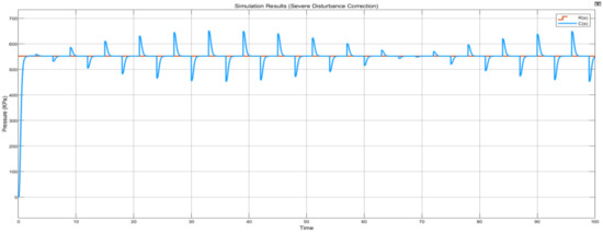
Figure 36. Severe disturbance plot.

In addition to the robust disturbance correction controller capability, it is apparent that the steady-state error is quickly achieved in both cases. This is ideal because it illustrates the controller’s capabilities in maintaining the desired operating conditions.

4. Implications

Hitherto, micro-controllers have not been applied in the context of driving acoustic horns. Normally, acoustic horns are operated through a solid-state electronic timer or sequence controller coupled onto a solenoid valve. The solid-state electronic timer has variable timing ranges to automatically control the solenoid valve that drives the acoustic horn [23]. Furthermore, the typical system configuration is only enabled for pressure activation and operation without the capability of varying supply pressure as deduced by the end use. Table 18 illustrates the typical main acoustic system components that are critical to the effectiveness of the acoustic horn.

Table 18. Acoustic system components [24].

Component	Recommendation
Solenoid valves	1 per horn, 1 per system
Manual isolation valve	1 per horn, 1 per system
Flow regulator	Air type based regulator
Flex	Stainless steel material

Considering the common industry practice for acoustic cleaning systems which implement PLCs, manual ball valves, or relays for the control operation, this paper has demonstrated novelty by introducing a micro-controller to drive the sonic horn. The micro-controller is also a feedback system that is capable of rejecting disturbances and also ensures that the controlled variable C(s) is the same as the reference signal R(s), which manual ball valves and relays are not capable of achieving. Another point of consideration is the introduction of alternate subsystems to facilitate accurate control actions. Table 19 illustrates the replacement components relative to the industry common configuration.

Table 19. Research novelty subsystem comparison.

Industry Standard Configuration	Research System Components
Solid-state electronic timer	I-P transducer
Solenoid valve	Spring and diaphragm valve
No feedback transducer	Piezoresistive pressure sensor
Industry Standard Configuration	Research System Components

5. Conclusions

The control system analysis and design were based on three objectives: transient response, steady-state error, and stability. Following the design philosophy in a sequential order, physical systems and specifications were determined. The requirement was that the acoustic horn should produce a sound frequency of 75 Hz at a pneumatic pressure of 552 kPa in order to clean the boiler tubes. The system was identified to have four (4) hardware parts, namely, I-P transducer, spring and diaphragm valve, acoustic horn, and a piezoelectric pressure sensor. A functional block diagram of the entire control system configuration was drawn to translate a qualitative account of the physical system. The block schematic representation described the system component parts and their interconnection.

Mathematical modelling of each subsystem was based on physical laws. For electrical networks, Kirchhoff’s current law was considered. For mechanical systems, Newton’s second law of motion was considered. In addition to estimating each subsystem’s behaviour, necessary logical means and simplifying assumptions were made to identify physical properties. The approximated continuous-time transfer functions of the hardware parts in concern were concluded as: I-P transducer ${\mathrm{G}}_{1^{\left(\mathrm{s}\right)}}$, spring and diaphragm valve ${\mathrm{G}}_{2^{\left(\mathrm{s}\right)}}$, acoustic horn ${\mathrm{G}}_{3^{\left(\mathrm{s}\right)}}$, and piezoelectric pressure sensor ${\mathrm{H}}_{\left(\mathrm{s}\right)}$.

Multiple subsystems were reduced to a corresponding singular block, with an equivalent transfer function labelled ${\mathrm{Final}}_{\mathrm{sys}}$. Following the block diagram reduction, a PID controller block was introduced into the system for analysis and design. The tuned controller gains enabled the required specifications and performance requirements of the control system to be met. This was demonstrated through testing and simulation environments, thereby satisfying the analysis and design objectives. The control system was proven to be stable with an ideal transient response of 0.562 s, while the steady-state error was attained in 1.05 s.

References

- Canete, J.; Cipriano, G.; Inmaculada, M. Introduction to Control Systems; Research Gate; Elsevier: Amsterdam, The Netherlands, 2011. [Google Scholar]
- Nise, N.S. Control Systems Engineering, 6th ed.; John Wiley & Sons Inc.: Pomona, CA, USA, 2010. [Google Scholar]
- Antsaklis, P.; Zhiqiany, G. The Electronics Engineers’ Handbook, 5th ed.; McGraw-Hill: New York, NY, USA, 2005. [Google Scholar]
- Bhattacharya, S.K. Control Systems Engineering, 2nd ed.; Pearson Education: Delhi, India, 2008. [Google Scholar]
- Mhlongo, B.; Kallon, D.V.V. Acoustics Vibration Sensing and Control Mechanism for Boilers. In Proceedings of the International Conference on Industrial Engineering and Operations Management, Singapore, 7–11 March 2021; pp. 4510–4522. [Google Scholar]
- Sivanandam, S.N.; Deepa, S.N. Control Systems Engineering Using Matlab, 2nd ed.; Vikas Publishing House: Delhi, India, 2009. [Google Scholar]
- Lewis, P.H.; Yang, C. Basic Control Systems Engineering; Prentice Hall: Hoboken, NJ, USA, 1997. [Google Scholar]
- Shandu, P.M. Design of an Acoustic Cleaning Apparatus for a Boiler at Sasol Synfuels Power Station in Secunda. Master’s Thesis, University of Johannesburg, Johannesburg, South Africa, 2020. [Google Scholar]
- Sinha, A. Vibration of Mechanical Systems; Cambridge: New York, NY, USA, 2010. [Google Scholar]
- Ryder, G.H.; Bennett, M.D. Mechanics of Machines; Industrial Press: New York, NY, USA, 1990. [Google Scholar]
- 657 and 667 Actuators. Available online: https://www.emerson.com/documents/automation/product-bulletin-fisher-657-667-diaphragm-actuators-en-122352.pdf (accessed on 15 October 2021).
- Shandu, P.M.; Kallon, D.V.V. A Case of Acoustics Cleaning of Industrial Boilers at Sasol Synfuels Power Station in Secunda. In Proceedings of the International Conference on Industrial Engineering and Operations Management, Sao Paulo, Brazil, 5–8 April 2021. [Google Scholar]
- De Silva, C.W. Vibration Damping, Control, and Design; CRC Press: Boca Raton, FL, USA, 2019. [Google Scholar]
- Baz, A.M. Active and Passive Vibration Damping; Wiley: Hoboken, NJ, USA, 2019. [Google Scholar]
- Saxby, G. Practical Holography, 3rd ed.; CRC Press: Philadelphia, PA, USA, 2003. [Google Scholar]
- Lamnabhi-Lagarrigue, F. Advanced Topics in Control Systems Theory: Lecture Notes from FAP 2004; Springer: London, UK, 2004. [Google Scholar]
- Palani, S. Control System Engineering, 2nd ed.; Tata McGraw Hill: New Delhi, India, 2010. [Google Scholar]
- Boiler Cleaning Methods & Techniques. Available online: https://www.power-eng.com/news/boiler-cleaning-methods-techniques/#gref (accessed on 2 September 2019).
- Levine, W.S. The Control Handbook; CRC Press: Boca Raton, FL, USA, 1996. [Google Scholar]
- Shandu, P.M.; Kallon, D.V.V.; Tartibu, L.K.; Mutyavavire, R. Development Design of an Acoustic Cleaning Apparatus for Boilers at Sasol Synfuels Power Station plant in Secunda. In Proceedings of the South African Computational and Applied Mechanics, Vanderbijlpark, South Africa, 17–19 September 2019. [Google Scholar]
- Machowski, J.; Lubosny, Z.; Bialek, J.W.; Bumby, J.R. Power System Dynamics: Stability and Control, 3rd ed.; Wiley: Hoboken, NJ, USA, 2020. [Google Scholar]
- Åström, K.J.; Hägglund, T. Advanced PID Control; ISA—The Instrumentation, Systems, and Automation Society: Pittsburgh, PA, USA, 2006. [Google Scholar]
- Acoustic Clean. Available online: https://controlconceptsusa.com/wp-content/uploads/2020/04/AcoustiClean-Sonic-Horn-Installation-Instructions.pdf (accessed on 2 April 2022).
- Acoustic Sonic Horns for Solving Material Handling Problems. Available online: http://filterbaglady.com/acoustic-horns/ (accessed on 2 April 2022).
Publisher’s Note: MDPI stays neutral with regard to jurisdictional claims in published maps and institutional affiliations. |
© 2022 by the authors. Licensee MDPI, Basel, Switzerland. This article is an open access article distributed under the terms and conditions of the Creative Commons Attribution (CC BY) license (https://creativecommons.org/licenses/by/4.0/).