Abstract
This study evaluates the effect of simple data-level balancing techniques on predicting school dropout across all state public high schools in Espírito Santo, Brazil. We trained Logistic Regression with LASSO (LR), Random Forest (RF), and Naive Bayes (NB) models on first-quarter data from 2018–2019 and forecasted dropouts for 2020, with additional validation in 2022. Facing strong class imbalance, we compared three balancing methods—RUS, SMOTE, and ROSE—against models trained on the original data. Performance was assessed using accuracy, sensitivity, specificity, precision, F1, AUC, and G-mean. Results show that the imbalance severely harmed RF and NB trained without balancing, while Logistic Regression remained more stable. Overall, balancing techniques improved most metrics: RUS and ROSE were often superior, while SMOTE produced mixed results. Optimal configurations varied by year and metric, and RUS and ROSE made up most of the best combinations. Although most configurations benefited from balancing, some decreased performance; therefore, we recommend systematic testing of multiple balancing strategies and further research into SMOTE variants and algorithm-level approaches.
1. Introduction
School dropout, defined as the premature interruption of formal education, arises from a complex interplay of socioeconomic, personal, and institutional factors. Dropping out of school has several negative consequences. At the individual level, it limits earning potential, employability, and social mobility. At the macroeconomic level, it impacts the distribution of human capital, contributing to income inequality and hindering socioeconomic advancement, thus perpetuating cycles of poverty and inequality [1]. As UNICEF [2] notes, disrupting the educational process deprives children and adolescents of the essential skills necessary to develop their potential, achieve economic independence, and actively participate in society. School dropout is also associated with a range of social problems, including a lower quality of life, poor health, and gender inequality. Furthermore, Wood et al. [3] highlight that high school dropout has been associated with higher rates of unemployment, incarceration, and mortality.
Developing early warning systems for dropout identification empowers educators by facilitating the identification of at-risk students. This, in turn, allows educators to plan effective interventions to mitigate this serious problem. Such models have been successfully implemented worldwide [4,5,6,7], and their importance is underscored by [2].
One of the inherent challenges in predicting student dropout is the imbalance between classes. The number of students who drop out is typically much lower than those who remain in school, creating a significant data imbalance. As Fernández et al. [8] point out, this imbalance can negatively impact predictive performance. According to Chen et al. [9], classification models typically assume a balanced class distribution. However, class imbalance poses a challenge, as traditional algorithms tend to favor more frequent classes, potentially neglecting the less common ones. This imbalance leads to a variation in the performance of the learning algorithms, known as performance bias [9].
To address the challenges posed by imbalanced datasets, numerous methodologies have been proposed, intervening at different stages of the modeling process. These solutions can be broadly classified into data-level approaches, algorithm-level techniques, or hybrid strategies [9,10].
Data-level approaches directly modify the training data to rebalance class distributions, often through techniques like oversampling minority classes or undersampling majority classes. A key advantage of these methods is their independence from specific learning algorithms, allowing easy integration with a variety of models [9]. However, Altalhan et al. [10] point out that this approach may discard potentially useful information or introduce noise through synthetic data.
Algorithm-level approaches, on the contrary, focus on adapting or developing machine learning algorithms to be more responsive to underrepresented groups [9]. Methods within this class encompass cost-sensitive learning, ensemble methods, and algorithm-specific adjustments [10]. While effective, these algorithms may not fully exploit the available data or may require complex adjustments for different algorithms. Finally, hybrid approaches strategically combine the advantages of both data-level and algorithm-level techniques to further improve performance. However, combining multiple techniques makes hybrid approaches complex, potentially leading to overfitting, increased computational demands, and a greater need for careful design. For a comprehensive overview of all possibilities to tackle imbalanced problems, see [9,10].
In this paper, we focus on data-level approaches for four reasons: (i) they can be used with any classifier; (ii) ease of implementation; (iii) direct control over class distribution; and (iv) widespread use, as indicated by the literature review. Numerous balancing techniques have been developed, including Random Undersampling (RUS), Synthetic Minority Oversampling Technique (SMOTE) [11], and Random Oversampling Examples (ROSE) [12], among others. SMOTE is frequently considered a benchmark balancing technique [9], as it attempts to address class imbalance by creating synthetic data points for the minority class.
Despite the inclination to use balancing techniques, some dropout classification models do not address the imbalance directly. These models, nevertheless, have demonstrated a satisfactory ability to identify at-risk students [13,14,15,16,17,18,19]. In contrast, other researchers automatically incorporate balancing methods into their dropout models [13,20,21]. Some have even investigated the best balancing method by comparing distinct approaches [22,23]. Still other works examine the efficiency of balancing methods by comparing models trained with and without these algorithms [24,25,26,27,28,29,30,31]. These studies suggest that the effect of the balancing methods is still an ongoing question.
A key conclusion from these works is that there is no universally optimal solution to the problem of imbalanced data. Some models built without balancing achieve strong results, while other studies find evidence supporting or refuting the use of balancing methods. Thus, testing various methods to choose the most appropriate for the data at hand would be the safest approach.
This research investigates the potential of simple balancing methods to improve the performance of classification models in predicting school dropouts for all state public high schools in Espírito Santo, Brazil, focusing on students in grades one, two, and three. Given the potential impact of imbalanced data on classifier performance, we tested three distinct balancing methods: RUS, SMOTE, and ROSE. RUS was chosen because of its simplicity and computational efficiency, while we chose SMOTE and ROSE to compare a traditionally used technique with an innovative one. While SMOTE is widely used and often considered a benchmark [8], ROSE offers a different approach by creating new data using statistical kernels, potentially expanding the decision region [12]. Furthermore, we noted a lack of applications of ROSE in the context of student dropout prediction. For classification in this study, we selected three prominent machine learning models: Logistic Regression (LR), Random Forest (RF), and Naive Bayes (NB). Logistic Regression was chosen for its inherent interpretability, allowing for a clear understanding of feature importance through its coefficients. Random Forest was selected for its ability to achieve high predictive accuracy by leveraging ensemble learning techniques. Finally, Naive Bayes was included due to its computational efficiency, ease of estimation, and demonstrated effectiveness in high-dimensional problems. These three models have been widely applied in the literature for predicting student dropout. We evaluated the performance of these classifiers after calibrating them with and without data balancing algorithms.
The results indicated that the inherent class imbalance in dropout data presents a significant challenge to effective model training. However, results also demonstrated that data balancing techniques, particularly RUS and ROSE, can improve model performance in terms of the majority of the metrics considered. While LR exhibits notable stability across different balancing techniques, RF models show greater variability, with RUS and ROSE generally producing the best results. Ultimately, we highlight the importance of carefully considering class imbalance and selecting appropriate balancing techniques, as the optimal choice may vary depending on the academic year and performance metric.
2. Related Works: The Role of Balancing Techniques in Predicting School Dropout
The development of accurate and reliable prediction models is crucial for implementing timely interventions and mitigating the negative consequences of school dropout. A recurring challenge is the inherent class imbalance in dropout datasets, where the number of non-dropout students significantly exceeds that of dropout students. This imbalance can negatively impact the performance of machine learning models, leading to biased predictions and reduced effectiveness in identifying at-risk students [8].
2.1. Dropout Prediction Without Explicit Balancing
Despite the challenges of unbalanced data, several studies have successfully developed predictive models for school dropout without explicitly addressing this issue.
For example, Sara et al. [14] compared the performance of Random Forest (RF), CART, Support Vector Machines (SVM), and Naive Bayes (NB) for secondary education in Denmark. In Honduras and Guatemala, Adelman et al. [15] employed a linear probability model. Sandoval-Palis et al. [16] tested Logistic Regression (LR) and Artificial Neural Networks (ANN) at Escuela Politécnica Nacional in Ecuador. Freitas et al. [17] compared LR, Decision Trees, and other machine learning methods at the Federal Institute of Education, Science, and Technology of Ceará (IFCE), Fortaleza campus, Brazil. Martinha et al. [32] developed a fuzzy ARTMAP neural network for the identification of dropout in technology courses at the Federal Institute of Mato Grosso, Brazil. Unlike these models that did not address the problem of unbalanced data, Rabelo and Zárate [19] proposed an ensemble model to predict higher education student dropout in a private institution in Brazil.
These studies highlight the potential of certain algorithms to implicitly handle class imbalance to some extent or the possibility that the specific characteristics of their datasets minimize the impact of the imbalance. However, these approaches may not be universally applicable, and their performance could be further improved by explicitly addressing the issue of class imbalance.
2.2. Balancing Techniques in Dropout Prediction
Recognizing the potential limitations of models trained on imbalanced data, numerous researchers have incorporated balancing techniques into their methodologies. Marquez-Vera et al. [13] developed an Interpretable Classification Rule Mining model with Grammar-based Genetic Programming and compared it with classifiers in Weka, jointly with SMOTE, to predict student dropout at the Autonomous University of Zacatecas in México. Rovira, Puertas, and Igual [20] also applied SMOTE to balance their data before training traditional machine learning models to predict student dropout at the University of Barcelona, Spain. Del Bonifro et al. [21] used random sampling to balance their dataset and then compared different machine learning methods. These studies demonstrate the increasing interest in the use of balancing techniques to improve the robustness of dropout prediction models.
2.3. Comparative Studies on Balancing Methods
A more focused research line involves comparing different balancing methods to identify the most effective approach for specific dropout prediction scenarios. Selim and Rezk [22] compared eight undersampling techniques, four oversampling techniques, and their mixed pairs in an Egyptian survey dataset, finding that ROS combined with NearMiss-3 improved F1 score and type II error performance. Villar and Andrade [23] evaluated supervised and unsupervised machine learning algorithms to predict dropout and academic success, focusing on the impacts of SMOTE and ADASYN, and found that SMOTE significantly improved the accuracy of the model.
2.4. Mixed Evidence on the Effectiveness of Balancing
Despite the growing body of research on balancing techniques, the evidence regarding their effectiveness remains mixed. Lee and Chung [25] employed SMOTE with traditional ML models to analyze a large dataset of high school students in South Korea and found ambiguous results, with some metrics indicating that balancing methods may or may not improve performance. Similarly, Costa et al. [24] found that balancing methods improved the quality of identification for online courses but had the opposite effect in face-to-face courses at a Brazilian public university. Barros et al. [26] found that data balancing techniques significantly increased the performance of predictive models in Integrated Education (secondary education with training in professional education) of the Federal Institute of Rio Grande do Norte, Brazil, while Orooji and Chen [27] found that imbalanced learning methods can produce good recall results but decrease precision, whereas classifiers without balanced data give better precision but poor recall.
More recently, Cho, Yu, and Kim [29] found that the performance of most models decreased after applying oversampling techniques, while Psathas, Chatzidaki, and Demetriadis [30] found that oversampling may significantly improve performance, but that different combinations of classification methods and balancing algorithms should be tested. In the same line, Kim et al. [31] proposed a student dropout prediction system for Gyeongsang National University, South Korea, and tested several combinations of balancing algorithms and machine learning classification methods. Wongvorachan, He, and Bulut [28] compared several balancing sampling techniques using the High School Longitudinal Study of 2009 from the United States of America and found that ROS for moderately imbalanced data and hybrid resampling for highly imbalanced data seem to work best.
The existing literature presents a complex and sometimes contradictory picture of the effectiveness of balancing techniques in the prediction of dropout. Although some studies demonstrate significant improvements in model performance, others find little or no benefit, or even negative impacts. This suggests that the optimal approach may depend on the specific characteristics of the dataset, the choice of machine learning algorithm, and the balancing technique employed. Furthermore, there is a notable lack of research on the application of certain balancing techniques, such as ROSE, in the context of student dropout prediction.
Therefore, this research aims to address this gap by systematically evaluating the impact of three different balancing methods (RUS, SMOTE, and ROSE) on the performance of Logistic Regression, Random Forest, and Naive Bayes models to predict school dropout in all public high schools in the state of Espírito Santo, Brazil. By comparing the performance of these models with and without balancing, we seek to provide valuable insights into the effectiveness of different approaches for handling class imbalance in dropout prediction and to identify the most suitable strategies for our specific context.
3. Methodology
In this section, we present the classifiers used (LR, RF, and NB), as well as a brief introduction to the balancing methods employed (RUS, SMOTE, and ROSE). The dependent variable is defined as , where 1 represents the dropout and 0 otherwise. As predictors, we used a set of personal information, school infrastructure, and administrative data regarding student performance and attendance during the first quarter of the year. The goal is to forecast whether the student may drop out during the entire year. Table 1 lists all the predictors considered.

Table 1.
Considered variables.
It is important to note that several models were estimated. Some were calibrated using the original imbalanced data, while others were trained with data balanced using the methods employed in this research. For this reason, for each specific grade of secondary school, twelve configurations were tested: (I) LR with LASSO, calibrated using the original imbalanced data; (II) RF, calibrated with the original data (imbalanced); (III) NB, calibrated with the original data (imbalanced); (IV) LR with LASSO, calibrated using RUS; (V) RF, calibrated with RUS; (VI) NB, calibrated with RUS; (VII) LR with LASSO, calibrated with SMOTE; (VIII) RF, calibrated with SMOTE; (IX) NB, calibrated with SMOTE; (X) LR with LASSO, calibrated with ROSE; (XI) RF, calibrated with ROSE; (XII) NB, calibrated with ROSE.
3.1. Classifiers
3.1.1. Logistic Regression
Logistic Regression is a common classifier and has been applied to several classification problems, such as dropout forecasting [18,20,29], credit risk prediction [33,34], bankruptcy prediction [35], oil market efficiency [36], and other applications. Mathematically, considering a binary dependent variable , the logistic regression is given by the following
where is a constant, is a column vector of coefficients, is a column vector of k predictors, and represents the linear combination of predictor variables. We used Logistic Regression in conjunction with the LASSO (least absolute shrinkage and selection operator), a technique used to select relevant variables. The primary advantage is the simultaneous estimation of model parameters and selection of the most relevant variables, while discarding irrelevant ones. Formally, the log-likelihood function is given by the following:
where indicates the sample size, and is the tuning parameter that controls the shrinkage, usually obtained by k-fold cross-validation. For more details, see [37,38]. In this research, we employed 5-fold cross-validation to select both the optimal hyperparameters (by minimizing the area under the ROC curve) and the probability threshold for converting predictions into binary outcomes.
3.1.2. Random Forest
Random Forests are tree-based ensemble methods built on the concept of stratification and segmenting predictor space [37]. They can be used for regression and classification problems [37,38]. Applications of RF are, for instance, credit modeling [33,34], dropout identification [20,29], stock market trading prediction [39], water temperature forecasting [40], and others. In essence, Random Forests aggregate a large number of Decision Trees and combine their individual predictions to obtain a final classification or prediction. Bootstrap and other ensemble methods are commonly employed in the construction of these trees.
Calibrating a Random Forest model typically involves tuning three key hyperparameters: the number of trees (), the minimum node size (), and the number of features sampled at each split (). The number of trees determines the size of the ensemble, with too few trees potentially limiting the ability to capture complex patterns and too many trees potentially leading to overfitting [41]. The number of features sampled at each split controls the randomness of the model, promoting diversity among the trees. The minimum node size dictates the minimum number of observations required in a terminal node to be considered for further splitting [42].
We employed a grid search to explore different hyperparameter values and compute the error on the validation set, with 5-fold cross-validation to find the optimal hyperparameters by minimizing the area under the ROC curve. We ran tests with a sequence of trees in intervals of 100, ranging from 100 to 1000, and fitted the best model using the caret package in R [43]. The hyperparameter mtree was selected in intervals of 1, ranging from 1 to the total number of variables minus one. Finally, the node size varied from 1 to 20.
3.1.3. Naive Bayes
According to [38], the Naive Bayes classifier is particularly suitable for high-dimensional explanatory variables. The applications of NB models are, for instance, in dropout forecasting [14], lemon disease detection [44], basketball game outcomes [45], and medical problems [46], among others. It is based on Bayes’ theorem, which, for a binary classification problem where and , states the following:
To apply this theorem, we can use training data to estimate and . These estimates then allow us to determine for any new instance of the predictor vector . However, estimating the distribution related to can be challenging, especially in high-dimensional spaces. The Naive Bayes Classifier addresses this challenge by making a key assumption: given a class Y, the features in are conditionally independent. This simplification allows the classifier to estimate the class-conditional marginal densities separately for each feature. For continuous features, this is typically performed using one-dimensional kernel density estimation. For discrete predictors, an appropriate histogram estimate can be used [38]. Under this independence assumption, Equation (3) can be rewritten as follows:
In this research, we employed a grid search approach for hyperparameter tuning of the Naive Bayes model. The tuned hyperparameters included the bandwidth of the kernel density estimation and the Laplace smoothing parameter, which addresses the issue of zero probabilities for unseen categories during training. To ensure robust model evaluation and selection, we implemented a 5-fold cross-validation procedure. For the Naive Bayes model, we did not optimize a threshold for transforming probabilities into binary predictions.
3.2. Balancing Methods
In this section, we briefly introduce the methods employed in this research: the Random Undersampling (RUS), synthetic minority oversampling technique (SMOTE) [8,11], and random oversampling examples (ROSE) [12]. For a more comprehensive understanding of these methods, see [47,48].
Random Undersampling involves constructing a balanced sample by randomly removing individuals from the majority class, thereby reducing its size while preserving all elements of the minority class. This approach decreases the overall sample size. Figure 1 illustrates this simple approach.
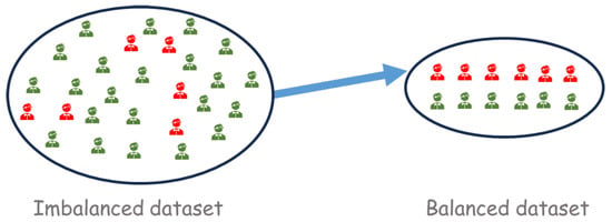
Figure 1.
Example of a balanced sample. The green elements are eliminated via random sampling. The resulting sample contains, in general, the same number of elements from both classes. After this step, we can estimate the classifier based on a balanced dataset.
Chawla et al. [11] proposed the SMOTE, which interpolates neighboring elements of the minority class to create synthetic elements. Consequently, the algorithm augments the minority class by incorporating simulated data while randomly removing elements from the majority class. According to the authors, this approach results in a larger and less specific decision region, thus enhancing the quality of the estimation. Figure 2 illustrates the construction of the final sample.
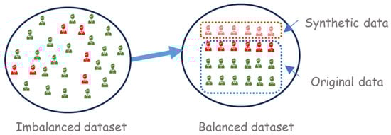
Figure 2.
An example of a balanced sample using SMOTE. The elements represented by the light red colour are generated via SMOTE and added to the dataset. Simultaneously, some elements of the majority class are discarded through random sampling.
While SMOTE effectively addresses class imbalance by generating synthetic minority class instances, it suffers from key limitations highlighted [9,15]. The potential for generating duplicate synthetic samples, especially within complex or overlapping datasets, can lead to redundancy and overfitting. Furthermore, original SMOTE overlooks the underlying data distributions, potentially creating synthetic samples that do not accurately represent the true minority class and are not well-suited for high-dimensional data. To address these shortcomings, numerous variations of SMOTE have been developed, such as Borderline-SMOTE, ADASYN, SMOTE-N, among others [10,29].
The ROSE was proposed by [12] and is based on the principles of SMOTE. The main distinction lies in the generation of the synthetic. In ROSE, the authors replace the interpolation technique with statistical kernels, thus overcoming SMOTE’s drawback of neglecting the underlying data distribution. This enables an expansion of the decision region beyond interpolation, resulting in newly generated data that differs from the original but remains statistically equiprobable. As a result, the decision region is expanding [12].
4. Experiments
4.1. Dataset
The dataset used in this study comprises variables collected from the Sistema Estadual de Gestão Escolar do Espírito Santo (SEGES) (State School Management System of Espírito Santo, translated freely) and the Instituto Nacional de Estudos e Pesquisas Educacionais Anísio Teixeira (INEP) (National Institute for Education Studies and Research Anísio Teixeira, translated freely). Table 1 lists all 49 variables used.
The objective is to classify students for the 2020 academic year, using data acquired shortly after the conclusion of the first academic quarter. This classification enables the calculation of student dropout probabilities during 2020 for students enrolled in the first, second, and third years of high school across all state schools in Espírito Santo, Brazil. To this end, the model was calibrated using data from the first academic quarters of 2018 and 2019. Furthermore, the calibrated model was also employed to forecast the dropout rate for 2022, thereby evaluating the predictive accuracy of the model against two distinct datasets. The results for 2022 are presented in Appendix A.1 through Table A1, Table A2, Table A3 and Table A4.
4.2. Results
The methods described above were used to forecast student dropout in 2020 for the first, second, and third years of high school in all public state schools in Espírito Santo, Brazil. To assess whether balancing methods improve forecasting metrics, we estimated twelve distinct models for each grade: (I) LR with LASSO, calibrated using the original imbalanced data; (II) RF, calibrated with the original data (imbalanced); (III) NB, calibrated with the original data (imbalanced); (IV) LR with LASSO, calibrated using RUS; (V) RF, calibrated with RUS; (VI) NB, calibrated with RUS; (VII) LR with LASSO, calibrated with SMOTE; (VIII) RF, calibrated with SMOTE; (IX) NB, calibrated with SMOTE; (X) LR with LASSO, calibrated with ROSE; (XI) RF, calibrated with ROSE; (XII) NB, calibrated with ROSE. The results presented in this section refer to models calibrated with data from 2018 and 2019, with the aim of forecasting dropout in 2020. In addition to this dataset, we also used the same calibrated models to predict school dropout in 2022. The results of this second exercise are presented in the Appendix A.1.
Table 2 displays the number of dropouts and non-dropouts in our data set for the first, second, and third years of high school in 2018, 2019, and 2020. As can be observed, the dataset shows a significant class imbalance.
Table 2.
Number of dropouts and non-dropouts in our dataset.
Table 3 and Figure 3 present the results for all twelve models. The highest value for each metric is highlighted in bold. The metrics for RF, NB, and RF with SMOTE models were not considered, as these models have significant limitations in accurately identifying dropout cases. The mathematical definition of each metric is based on the confusion matrix (Table A5) and ROC curve (Figure A1). For more details, see Appendix A.2. Comparing the three models estimated with the original data—LR, RF, and NB—it is evident that RF and NB struggled to identify students at risk of dropping out, exhibiting sensitivities approaching or reaching zero. This also prevented the calculation of precision and F1 scores for the RF. This issue stemmed from the severe imbalance in the data set, as shown in Table 2. The LR model performed better with the imbalanced data, achieving a sensitivity of 0.791 and an AUC of 0.819.
Table 3.
Metrics for the first year of high school in 2020.
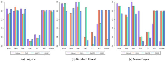
Figure 3.
Metrics for the first year of high school. Each group of bars represents the results of the four models evaluated across all metrics considered: accuracy (Accur.), sensitivity (Sens.), specificity (Spec.), precision (Prec.), area under the ROC curve (AUC), and G-mean. The metrics are presented in a tripartite layout: LR classifier results on the left, RF in the center, and NB on the right.
When training the models with balanced data, we observed an increase in sensitivity across all models, except for the RF with SMOTE. The RF with SMOTE still faced considerable challenges in identifying students who dropped out, with a sensitivity of only 0.021. This resulted in very high accuracy (0.967) and perfect specificity, but at the expense of practical usefulness for identifying at-risk students.
Taking into account the F1, AUC, and G-mean metrics, which are commonly used for imbalanced datasets and when looking for a metric that balances different aspects of model performance, the best results were achieved by NB with SMOTE, RF with ROSE, and RF with ROSE, respectively. The metrics were for NB SMOTE (F1: 0.318, AUC: 0.788, and G-mean: 0.788) and RF with ROSE (F1: 0.215, AUC: 0.822, and 0.821), respectively. While AUC scores varied across most models, the differences were relatively small (ranging from 0.778 to 0.822). Notable exceptions were the RF trained on the original and SMOTE-balanced data and the NB model trained on the original data, all of which exhibited poor performance. The LR and NB models demonstrated notable stability across different data balancing techniques, with AUC scores ranging from 0.778 to 0.821 and 0.788 to 0.806, respectively, indicating low variance in performance. In contrast, the Random Forest (RF) models exhibited high variability, performing well with RUS and ROSE but poorly with the original data and SMOTE.
Taking into account the results for the second year of high school, Figure 4 and Table 4 show the results for the twelve models. The highest value for each metric is highlighted in bold, following the criterion adopted in Table 3. Comparing the LR, RF, and NB models trained on the original (unbalanced) data, we observed a similar pattern to that found in the first grade. The RF and NB models again exhibited poor performance in identifying at-risk students, with near-zero sensitivity. However, the LR model performed substantially better on the imbalanced data, achieving AUC and G-mean values of 0.855 and 0.854, respectively. Furthermore, LR with RUS yielded the best F1-score.
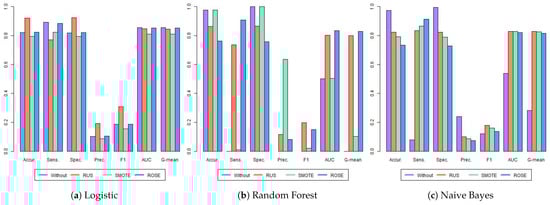
Figure 4.
Metrics for the second year of high school. Each group of bars represents the results of the four models evaluated across all metrics considered: accuracy (Accur.), sensitivity (Sens.), specificity (Spec.), precision (Prec.), area under the ROC curve (AUC), and G-mean. The metrics are presented in a tripartite layout: LR classifier results on the left, RF in the center, and NB on the right.
Table 4.
Metrics for the second year of high school in 2020.
Finally, Table 5 and Figure 5 present the results for the third year of high school for 2020. Using the original imbalanced data, the LR model maintained a similar level of performance as in the first and second grades, with an accuracy of 0.806, sensitivity of 0.852, and AUC of 0.829. This consistency suggests the LR model is robust across different high school grades. In contrast, the RF and NB models continued to perform poorly on the original data, exhibiting near-zero sensitivity. This mirrors the findings from previous grades, suggesting that RF and NB models struggle to identify at-risk students when the data is highly imbalanced.
Table 5.
Metrics for the third year of high school in 2020.
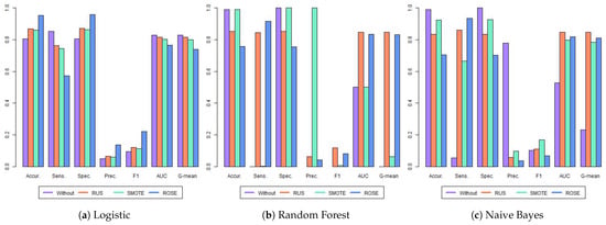
Figure 5.
Metrics for the third year of high school. Each group of bars represents the results of the four models evaluated across all metrics considered: accuracy (Accur.), sensitivity (Sens.), specificity (Spec.), precision (Prec.), area under the ROC curve (AUC), and G-mean. The metrics are presented in a tripartite layout: LR classifier results on the left, RF in the center, and NB on the right.
When applying the balancing techniques, we found that the highest AUC was achieved by the RF with RUS. Conversely, the best accuracy, specificity, precision, and F1 were attained by LR with ROSE. Regarding G-mean, there is a tie between the two models (RF with RUS and NB with RUS). Once again, Random Forest with SMOTE showed a poor performance in identifying dropouts.
Table 6 presents the optimal configuration for each metric and academic year. As observed, data balancing techniques improved the majority—approximately 95%—of the metrics analyzed. The only exception was the AUC and the G-mean metric for the second year of high school, which showed no improvement with any balancing methods.
Table 6.
Optimal configuration for each metric in 2020.
Considering only the best-performing configurations, models without balancing algorithms achieved the top result in just 10% of cases. SMOTE was among the best in 19% of the cases, RUS in 33%, and ROSE in 38%. Regarding classifiers, LR was the most prevalent, appearing in 52% of the top configurations, while RF and NB comprised 23% and 28%, respectively.
4.3. Conclusions
This paper aims to evaluate the effect of data balancing algorithms on the performance of predictive models applied to a highly imbalanced education dataset. To achieve this goal, we explore three classification approaches (LR, NB, and RF) in conjunction with three balancing techniques (RUS, SMOTE, and ROSE). In addition, the classifiers were trained on the original unbalanced data, allowing a direct comparison of the effectiveness of each approach.
The methods described above were trained with data from the first quarter of 2018 and 2019 and, subsequently, were used for forecasting student dropout in 2020 for the first, second, and third grade of high school in all state schools in Espírito Santo, Brazil. In addition, as a second exercise, we also employed the same estimated models to forecast student dropout in 2022.
Our results demonstrated that the inherent class imbalance in dropout data poses a significant challenge to effective model training. In particular, the RF and the NB struggled to identify at-risk students when trained on the original imbalanced data, as evidenced by its low sensitivity.
However, the application of data balancing techniques, particularly RUS and ROSE, could improve the performance of the models. Restricting analysis to the optimal configurations identified, for the year 2020, Random Undersampling (RUS) was observed in 33% of instances, with ROSE present in 38%. The SMOTE algorithm was utilized in 19% of the configurations, while classifiers trained directly on imbalanced data yielded superior results in only 10% of cases. In 2022, the optimal strategies consisted exclusively of ROSE (24%) and RUS (76%).
The findings of this study highlight the potential of balancing methods to improve predictive performance. However, choosing the best algorithm is not straightforward and depends on the metrics considered. In most cases, RUS and ROSE showed the best performance, but it is important to note that all methods could potentially decrease performance. This could be because the algorithms considered, such as those employing Random Undersampling, potentially discard valuable information from the majority class, hindering accurate estimation. Similarly, oversampling techniques risk generating duplicate or unrepresentative synthetic samples, particularly within complex or overlapping datasets. To address these limitations, further investigation into alternative data balancing techniques is recommended, with particular emphasis on techniques derived from SMOTE. Moreover, the exploration of algorithm-level methods for highly imbalanced data, such as cost-sensitive learning or ensemble methods, warrants further study. Future research should also consider exploring alternative modeling approaches tailored to imbalanced data. Specifically, testing different link functions within the framework of Logistic Regression presents a promising avenue for improvement. By employing link functions that better accommodate skewed class distributions, it may be possible to develop more robust and accurate classification models, minimizing the need for aggressive data balancing.
These findings have practical implications for the development of early warning systems for school dropout. The use of data balancing techniques and careful selection of the model can significantly improve the ability to accurately identify at-risk students, enabling targeted interventions. It is important to note that the optimal balancing technique can vary depending on the academic year and the specific performance metric. In general, this research underscores the importance of carefully considering class imbalance and selecting appropriate balance techniques for the development of accurate and effective school dropout prediction models.
Author Contributions
Conceptualization, G.A.d.A.P. and K.d.D.D.; methodology, G.A.d.A.P. and K.d.D.D.; software, G.A.d.A.P.; validation, G.A.d.A.P. and K.d.D.D.; formal analysis, G.A.d.A.P.; investigation, G.A.d.A.P. and K.d.D.D.; resources, G.A.d.A.P. and K.d.D.D.; data curation, G.A.d.A.P. and K.d.D.D.; writing—original draft preparation, G.A.d.A.P.; writing—review and editing, G.A.d.A.P. and K.d.D.D.; visualization, G.A.d.A.P.; supervision, K.d.D.D.; project administration, K.d.D.D.; funding acquisition, K.d.D.D. All authors have read and agreed to the published version of the manuscript.
Funding
This research was funded by the Espírito Santo Research and Innovation Support Foundation (FAPES), Department of Education of the State of Espírito Santo (SEDU-ES), and the Jones dos Santos Neves Institute (IJSN) through the Cooperation Agreement SEDU/IJSN/FAPES n° 015/2021, Grant Agreement FAPES and IJSN n° 141/2021, and CCAF Resolution n° 284/2021-Educational Studies.
Institutional Review Board Statement
Not applicable.
Informed Consent Statement
Not applicable.
Data Availability Statement
The dataset containing sensitive data was provided by the Secretariat of Education of Espírito Santo (SEDU-ES). The authors are not permitted to share this data. Requests for data access must be submitted through the official SEDU-ES website: https://sedu.es.gov.br.
Acknowledgments
The authors would also like to thank SEDU-ES for providing the data.
Conflicts of Interest
The authors declare that there are no competing interests.
Abbreviations
The following abbreviations are used in this manuscript:
| ANN | Artificial Neural Network |
| CART | Classification and Regression Trees |
| LR | Logistic Regression |
| RF | Random Forest |
| ROC | Receiver Operating Characteristic Curve |
| ROSE | Random Oversampling Examples |
| RUS | Random Undersampling |
| SMOTE | Synthetic Minority Oversampling Technique |
| SVM | Support Vector Machine |
Appendix A
Appendix A.1. Results for 2022
Table A1, Table A2 and Table A3 present the metrics for the first, second, and third years of high school in 2022. The purpose of this analysis is to verify whether the pattern observed in 2020 was repeated. As can be seen, RF, NB, and RF with SMOTE showed significantly lower predictive performance. Furthermore, the balancing methods were able to improve the metrics considered, with particular emphasis on RUS and ROSE.
Across all models and metrics, RUS was present in 76% of the best configurations, while ROSE appeared in only 24%. These two methods dominated the best-performing configurations. Regarding classifiers, LR appeared in 52% of cases, RF in 43%, and NB in only 5%.
Table A1.
Metrics for the first year of high school in 2022 for Logistic and Random Forest classifiers.
Table A1.
Metrics for the first year of high school in 2022 for Logistic and Random Forest classifiers.
| Classifier | Balancing | Accur. | Sens. | Spec. | Prec. | F1 | AUC | G-Mean |
|---|---|---|---|---|---|---|---|---|
| Logistic | - | 0.971 | 0.211 | 0.989 | 0.311 | 0.251 | 0.600 | 0.456 |
| RF | - | 0.977 | 0.000 | 1.000 | - | - | 0.500 | - |
| NB | - | 0.977 | 0.002 | 1.000 | 1.000 | 0.004 | 0.501 | 0.043 |
| Logistic | RUS | 0.975 | 0.150 | 0.995 | 0.399 | 0.218 | 0.572 | 0.385 |
| RF | RUS | 0.934 | 0.543 | 0.943 | 0.183 | 0.274 | 0.743 | 0.715 |
| NB | RUS | 0.955 | 0.475 | 0.967 | 0.251 | 0.328 | 0.721 | 0.678 |
| Logistic | SMOTE | 0.972 | 0.231 | 0.990 | 0.350 | 0.278 | 0.610 | 0.478 |
| RF | SMOTE | 0.977 | 0.000 | 1.000 | - | - | 0.500 | - |
| NB | SMOTE | 0.814 | 0.726 | 0.816 | 0.085 | 0.152 | 0.771 | 0.770 |
| Logistic | ROSE | 0.965 | 0.327 | 0.980 | 0.277 | 0.300 | 0.654 | 0.566 |
| RF | ROSE | 0.863 | 0.765 | 0.865 | 0.118 | 0.205 | 0.815 | 0.813 |
| NB | ROSE | 0.890 | 0.701 | 0.894 | 0.135 | 0.226 | 0.797 | 0.791 |
The highest value for each metric is highlighted in bold. The metrics for RF (without balacing), NB (without balacing), and RF with SMOTE models were not considered, as these models have significant limitations in accurately identifying dropout cases.
Table A2.
Metrics for the second year of high school in 2022 for Logistic and Random Forest classifiers.
Table A2.
Metrics for the second year of high school in 2022 for Logistic and Random Forest classifiers.
| Classifier | Balancing | Accur. | Sens. | Spec. | Prec. | F1 | AUC | G-Mean |
|---|---|---|---|---|---|---|---|---|
| Logistic | - | 0.916 | 0.683 | 0.922 | 0.182 | 0.287 | 0.803 | 0.793 |
| RF | - | 0.975 | 0.000 | 1.000 | - | - | 0.500 | - |
| NB | - | 0.975 | 0.019 | 1.000 | 0.579 | 0.036 | 0.509 | 0.137 |
| Logistic | RUS | 0.960 | 0.536 | 0.970 | 0.314 | 0.396 | 0.753 | 0.721 |
| RF | RUS | 0.852 | 0.813 | 0.853 | 0.123 | 0.213 | 0.833 | 0.832 |
| NB | RUS | 0.801 | 0.783 | 0.801 | 0.091 | 0.162 | 0.792 | 0.792 |
| Logistic | SMOTE | 0.958 | 0.510 | 0.969 | 0.296 | 0.374 | 0.740 | 0.703 |
| RF | SMOTE | 0.975 | 0.024 | 0.999 | 0.378 | 0.045 | 0.511 | 0.154 |
| NB | SMOTE | 0.616 | 0.911 | 0.609 | 0.056 | 0.105 | 0.760 | 0.745 |
| Logistic | ROSE | 0.930 | 0.659 | 0.937 | 0.210 | 0.318 | 0.798 | 0.786 |
| RF | ROSE | 0.705 | 0.913 | 0.700 | 0.071 | 0.132 | 0.806 | 0.799 |
| NB | ROSE | 0.749 | 0.897 | 0.745 | 0.082 | 0.150 | 0.821 | 0.817 |
The highest value for each metric is highlighted in bold. The metrics for RF (without balacing), NB (without balacing), and RF with SMOTE models were not considered, as these models have significant limitations in accurately identifying dropout cases.
Table A3.
Metrics for the third year of high school in 2022 for Logistic and Random Forest classifiers.
Table A3.
Metrics for the third year of high school in 2022 for Logistic and Random Forest classifiers.
| Classifier | Balancing | Accur. | Sens. | Spec. | Prec. | F1 | AUC | G-Mean |
|---|---|---|---|---|---|---|---|---|
| Logistic | - | 0.953 | 0.629 | 0.957 | 0.158 | 0.252 | 0.793 | 0.776 |
| RF | - | 0.987 | 0.000 | 1.000 | - | - | 0.500 | - |
| NB | - | 0.784 | 0.860 | 0.783 | 0.048 | 0.091 | 0.821 | 0.821 |
| Logistic | RUS | 0.977 | 0.482 | 0.983 | 0.265 | 0.342 | 0.732 | 0.688 |
| RF | RUS | 0.859 | 0.831 | 0.859 | 0.070 | 0.130 | 0.845 | 0.845 |
| NB | RUS | 0.716 | 0.932 | 0.713 | 0.040 | 0.076 | 0.822 | 0.815 |
| Logistic | SMOTE | 0.935 | 0.673 | 0.938 | 0.122 | 0.207 | 0.805 | 0.794 |
| RF | SMOTE | 0.986 | 0.022 | 0.999 | 0.176 | 0.038 | 0.510 | 0.146 |
| NB | SMOTE | 0.897 | 0.745 | 0.899 | 0.086 | 0.155 | 0.822 | 0.818 |
| Logistic | ROSE | 0.894 | 0.748 | 0.896 | 0.084 | 0.151 | 0.822 | 0.818 |
| RF | ROSE | 0.651 | 0.946 | 0.647 | 0.033 | 0.064 | 0.797 | 0.782 |
| NB | ROSE | 0.699 | 0.917 | 0.696 | 0.037 | 0.071 | 0.807 | 0.799 |
The highest value for each metric is highlighted in bold. The metrics for RF (without balacing), NB (without balacing), and RF with SMOTE models were not considered, as these models have significant limitations in accurately identifying dropout cases.
In Table A4, it is evident that balance was able to improve all metrics throughout the different high school years. Furthermore, the balancing methods ROSE and RUS proved to be the most effective. These results are similar to those previously observed.
Table A4.
Optimal configuration for each metric in 2022.
Table A4.
Optimal configuration for each metric in 2022.
| Metric | First Year | Second Year | Third Year |
|---|---|---|---|
| Accuracy | Logistic & RUS | Logistic & RUS | Logistic & RUS |
| Sensitivity | RF & ROSE | RF & ROSE | RF & ROSE |
| Specificity | Logistic & RUS | Logistic & RUS | Logistic & RUS |
| Precision | Logistic & RUS | Logistic & RUS | Logistic & RUS |
| F1 | NB & RUS | Logistic & RUS | Logistic & RUS |
| AUC | RF & ROSE | RF & RUS | RF & RUS |
| G-mean | RF & ROSE | RF & RUS | RF & RUS |
Appendix A.2. Evaluation Metrics
Most of the metrics employed in this research are based on the confusion matrix. Table A5 illustrates all possible classifications that our model can make. A true negative occurs when the model classifies the student as non-abandon, and they indeed do not leave the school. Conversely, a true positive happens when the model correctly identifies students who drop out. Errors occur in two situations: false positives and false negatives. In the former, the model classifies the student as abandoned, but they do not leave the school. False negatives occur when the model predicts the student as non-abandon, but they leave the school.
Table A5.
Confusion Matrix.
Table A5.
Confusion Matrix.
| Predicted 0 | Predicted 1 | |
|---|---|---|
| Actual 0 | TN (True Negative) | FP (False Positive) |
| Actual 1 | FN (False Negative) | TP (True Positive) |
Mathematically, the metrics are defined as:
- Accuracy: (TN + TP)/(TN + FP + FN + TP);
- Sensitivity: TP/(FN+TP);
- Specificity: TN/(TN+FP);
- Precision: TP/(TP+FP);
- F1-Score: 2TP/(2TP + FP + FN)
- G-mean:
Accuracy measures the percentage of correct classifications. Sensitivity measures the percentage of students who leave the school who were correctly identified. However, specificity is the percentage of students who do not leave the school and who were correctly identified. The precision is given by the proportion of correct classifications of dropout students divided by the total number of classifications equal to 1 made by the model. Finally, the F1-Score can be understood as a function of precision and sensitivity.
According to [10], accuracy and precision may not adequately capture de model performance in imbalanced datasets. The classifier may reach a relatively high accuracy even if that minority of categories are completely ignored [9]. For [10], AUC and F1-score are metrics more appropriated in imbalaced datasets, while [9] point out that AUC and G-mean are unaffected by imbalances in the class distribution.
In addition to these metrics, we employed the area under the receiver operating characteristic curve (AUC). A receiver operating characteristic curve (ROC curve) illustrates the relationship between the true and false positive rates for various threshold classifications. The AUC metric summarises the ROC curve by calculating the area under the curve, which ranges between 0 and 1. The greater the AUC, the better the classification. Figure A1 illustrates these concepts. In this figure the blue line represents the ROC curve itself. Each point on this curve corresponds to a specific classification threshold, showing the trade-off between the True Positive Rate and the False Positive Rate. The curve demonstrates how the classifier’s performance changes as the threshold for classifying a positive instance is varied. The red dashed line represents the line of no-discrimination (also known as random guess line). This line indicates the performance of a classifier that randomly guesses the class. An AUC of 1.0 represents a perfect classifier, while an AUC of 0.5 represents a classifier no better than random guessing.

Figure A1.
The ROC curve.
Figure A1.
The ROC curve.

References
- Burgess, S. Human Capital and Education: The State of Art in the Economics of Education; Technical Report; Institute for the Study of Labour: Bonn, Germany, 2016. [Google Scholar]
- UNICEF. Early Warning Systems for Students at Risk of Dropping Out; Unicef Series on Education Participation and Dropout Prevention; UNICEF: New York, NY, USA, 2017. [Google Scholar]
- Wood, L.; Kiperman, S.; Esch, R.C.; Leroux, A.J.; Truscott, S.D. Predicting dropout using student-and school-level factors: An ecological perspective. Sch. Psychol. Q. 2017, 32, 35. [Google Scholar] [CrossRef]
- Lamb, S.; Rice, S. Effective Strategies to Increase School Completion Report: Report to the Victorian Department of Education and Early Childhood Development; Technical Report; Communications Division, Department of Education and Early Childhood Development: Fredericton, NB, Canada, 2008. [Google Scholar]
- Knowles, J.E. Of needles and haystacks: Building and accurate statewide dropout early warnings system in Wisconsin. J. Educ. Data Min. 2015, 7, 18–67. [Google Scholar] [CrossRef]
- Uldall, J.S.; Rojas, C.G. An application of machine learning in public policy early warning prediction of school dropout in the Chilean public education system. Multidiscip. Bus. Rev. 2022, 15, 20–35. [Google Scholar] [CrossRef]
- Sletten, M.A.; Toge, A.G.; Malmberg-Heimonem, I. Effects of an early warning system on student absence and completion in Norwegian upper secondary schools: A cluster-randomised study. Scand. J. Educ. Res. 2022, 67, 1151–1165. [Google Scholar] [CrossRef]
- Fernández, A.; Garcia, S.; Herrera, F.; Chawla, N.V. SMOTE for learning from imbalanced data: Progress and challenges, marking the 15-year anniversary. J. Artif. Intell. Res. 2018, 61, 863–905. [Google Scholar] [CrossRef]
- Chen, W.; Yang, K.; Yu, Z.; Shi, Y.; Chen, C.P. A survey on imbalanced learning: Latest research, applications and future directions. Artif. Intell. Rev. 2024, 57, 137. [Google Scholar] [CrossRef]
- Altalhan, M.; Algarni, A.; Alouane, M.T.H. Imbalanced data problem in machine learning: A review. IEEE Access 2025. [Google Scholar] [CrossRef]
- Chawla, N.V.; Bowyer, K.W.; Hall, L.O.; Kegelmeyer, W.P. SMOTE: Synthetic minority over-sampling technique. J. Artif. Intell. Res. 2002, 16, 321–357. [Google Scholar] [CrossRef]
- Menardi, G.; Torelli, N. Training and assessing classification rules with imbalanced data. Data Min. Knowl. Discov. 2014, 28, 92–122. [Google Scholar] [CrossRef]
- Marquez-Vera, C.; Cano, A.; Romero, C.; Noaman, A.Y.M.; Fardoun, H.M.; Ventura, S. Early dropout prediction using data mining: A case study with high school students. Expert Syst. 2016, 33, 107–124. [Google Scholar] [CrossRef]
- Sara, N.B.; Halland, R.; Igel, C.; Alstrup, S. High-school dropout prediction using machine learning: A Danish large-scale study. In Proceedings of the ESANN 2015 Proceedings, European Symposium on Artificial Neural Networks, Computational Intelligence, Bruges, Belgium, 22–24 April 2015; p. 6. [Google Scholar]
- Adelman, M.; Haimovich, F.; Ham, A.; Vazquez, E. Predicting school dropout with administrative data: New evidence from Guatemala and Honduras. Educ. Econ. 2018, 26, 356–372. [Google Scholar] [CrossRef]
- Sandoval-Palis, I.; Naranjo, D.; Vidal, J.; Gilar-Corbi, R. Early dropout prediction model: A case study of university leveling course students. Sustainability 2020, 12, 9314. [Google Scholar] [CrossRef]
- Freitas, F.A.d.S.; Vasconcelos, F.F.; Peixoto, S.A.; Hassan, M.M.; Dewan, M.A.A.; Albuquerque, V.H.C.; Filho, P.P.R. IoT system for school dropout prediction using machine learning techniques based on socioeconomic data. Electronics 2020, 9, 1613. [Google Scholar] [CrossRef]
- Pereira, G.A.A.; Demura, K.D.; Nunes, I.C.; Paula, L.C.; Lira, P.S. An early warning system for school dropout in the state of Espírito Santo: A machine learning approach with variable selection methods. Pesqui. Oper. 2024, 44, 1–18. [Google Scholar] [CrossRef]
- Rabelo, A.M.M.; Zárate, L.E. A model for predicting dropout of higher education students. Data Sci. Manag. 2024; in press. [Google Scholar] [CrossRef]
- Rovira, S.; Puertas, E.; Igual, L. Data-driven system to predict academic grades and dropout. PLoS ONE 2017, 12, e0171207. [Google Scholar] [CrossRef] [PubMed]
- Del Bonifro, F.; Gabbrilelli, M.; Lisanti, G.; Zingaro, S.P.P. Student dropout prediction. In Artificial Intelligence in Education, Proceedings of the AIED 2020, Ifrane, Morocco, 6–10 July 2020; Lecture Notes in Computer Science; Bittencourt, I.I., Cukurova, M., Luckin, R., Millán, E., Eds.; Springer: Berlin/Heidelberg, Germany, 2020. [Google Scholar] [CrossRef]
- Selim, K.S.; Rezk, S.S. On predicting school dropouts in Egypt: A machine learning approach. Educ. Inf. Technol. 2023, 28, 9235–9266. [Google Scholar] [CrossRef]
- Villar, A.; Andrade, C. Supervised machine learning algorithms for predicting student dropout and academic success: A comparative study. Discov. Artif. Intell. 2024, 4, 2. [Google Scholar] [CrossRef]
- Costa, E.B.; Fonseca, B.; Santana, M.A.; de Araújo, F.F.; Rego, J. Evaluating the effectiveness of educational data mining techniques for early prediction of students’ academic failure in introductory programming courses. Comput. Hum. Behav. 2017, 73, 247–256. [Google Scholar] [CrossRef]
- Lee, S.; Chung, J.Y. The machine learning-based dropout early warning system for improving the performance of dropout prediction. Appl. Sci. 2019, 9, 3093. [Google Scholar] [CrossRef]
- Barros, T.M.; Neto, P.A.S.; Silva, I.; Guedes, L.A. Predictive models for imbalanced data: A school dropout perspective. Educ. Sci. 2019, 9, 275. [Google Scholar] [CrossRef]
- Orooji, M.; Chen, J. Predicting Louisiana public high school dropout through imbalanced learning yechniques. In Proceedings of the 2019 18th IEEE International Conference On Machine Learning And Applications (ICMLA), Boca Raton, FL, USA, 16–19 December 2019; IEEE: New York, NY, USA, 2019. [Google Scholar] [CrossRef]
- Wongvorachan, T.; He, S.; Bulut, O. A comparison of undersampling, oversampling, and SMOTE methods for dealing with imbalanced classification in educational data mining. Information 2023, 14, 54. [Google Scholar] [CrossRef]
- Cho, C.H.; Yu, Y.W.; Kim, H.G. A Study on dropout prediction for university students using machine learning. Appl. Sci. 2023, 13, 12004. [Google Scholar] [CrossRef]
- Psathas, G.; Chatzidaki, T.K.; Demetriadis, S.N. Learning, predictive modeling of student dropout in MOOCs and self-regulated. Computers 2023, 12, 194. [Google Scholar] [CrossRef]
- Kim, S.; Choi, E.; Jun, Y.; Lee, S. Student dropout prediction for university with high precision and recall. Appl. Sci. 2023, 13, 6275. [Google Scholar] [CrossRef]
- Martinho, V.; Nunes, C.; Minussi, C.R. An intelligent system for prediction of school dropout risk group in higher education classroom based on artificial neural networks. In Proceedings of the 2013 IEEE 25th International Conference on Tools with Artificial Intelligence, Herndon, VA, USA, 4–6 November 2013; IEEE: New York, NY, USA, 2013; pp. 159–166. [Google Scholar] [CrossRef]
- Bastos, J.A. Predicting credit scores with boosted decision trees. Forecasting 2022, 4, 925–935. [Google Scholar] [CrossRef]
- Souadda, L.I.; Halitim, A.R.; Benilles, B.; Oliveira, J.M.; Ramos, P. Optimizing credit risk prediction for peer-to-peer lending using machine learning. Forecasting 2025, 7, 35. [Google Scholar] [CrossRef]
- Papana, A.; Spyridou, A. Bankruptcy prediction: The case of the Greek market. Forecasting 2020, 2, 505–525. [Google Scholar] [CrossRef]
- Dimitriadou, A.; Gogas, P.; Papadimitriou, T.; Plakandaras, V. Oil market efficiency under a machine learning perspective. Forecasting 2019, 1, 157–168. [Google Scholar] [CrossRef]
- James, G.; Witten, D.; Hastie, T.; Tibshirani, R. An Introduction to Statistical Learning with Applications in R; Springer Series in Statistics; Springer: New York, NY, USA, 2013. [Google Scholar]
- Hastie, T.; Tibshirani, R.; Friedman, J. The Elements of Statistical Learning: Data Mining, Inference, and Prediction; Springer Series in Statistics; Springer: New York, NY, USA, 2017. [Google Scholar]
- King, J.C.; Amigó, J.M. Integration of LSTM networks in random forest algorithms for stock market trading predictions. Forecasting 2025, 7, 49. [Google Scholar] [CrossRef]
- Ptak, M.; Sojka, M.; Szyga-Pluta, K.; Amnuaylojaroen, T. Three environments, one problem: Forecasting water temperature in Central Europe in response to climate change. Forecasting 2025, 7, 24. [Google Scholar] [CrossRef]
- Breiman, L. Random forests. Mach. Learn. 2001, 45, 5–32. [Google Scholar] [CrossRef]
- Spiliotis, E.; Abolghasemi, M.; Hyndman, R.J.; Petropoulos, F. Hierarchical forecast reconciliation with machine learning. Appl. Soft Comput. 2021, 112, 107756. [Google Scholar] [CrossRef]
- Kuhn, M. Building predictive models in R using the caret package. J. Stat. Softw. 2008, 28, 1–26. [Google Scholar] [CrossRef]
- Ullah, N.; Ruocco, M.; Della Cioppa, A.; De Falco, I.; Sannino, G. An explainable deep learning framework with adaptive feature selection for smart lemon disease classification in agriculture. Electronics 2025, 14, 3928. [Google Scholar] [CrossRef]
- Alves, J.M.; Barbosa, R.S. Machine learning for basketball game outcomes: NBA and WNBA leagues. Computation 2025, 13, 230. [Google Scholar] [CrossRef]
- Changpetch, P.; Pitpeng, A.; Hiriote, S.; Yuangyai, C. Integrating data mining techniques for Naïve Bayes classification: Applications to medical datasets. Computation 2021, 9, 99. [Google Scholar] [CrossRef]
- He, H.; Garcia, E.A. Learning from imbalanced data. IEEE Trans. Knowl. Data Eng. 2009, 21, 1263–1284. [Google Scholar] [CrossRef]
- He, H.; Ma, Y. Imbalanced Learning: Foundations, Algorithms and Applications; IEEE Press—Wiley: Hoboken, NJ, USA, 2013. [Google Scholar]


Disclaimer/Publisher’s Note: The statements, opinions and data contained in all publications are solely those of the individual author(s) and contributor(s) and not of MDPI and/or the editor(s). MDPI and/or the editor(s) disclaim responsibility for any injury to people or property resulting from any ideas, methods, instructions or products referred to in the content. |
© 2025 by the authors. Licensee MDPI, Basel, Switzerland. This article is an open access article distributed under the terms and conditions of the Creative Commons Attribution (CC BY) license (https://creativecommons.org/licenses/by/4.0/).