Improvement on Forecasting of Propagation of the COVID-19 Pandemic through Combining Oscillations in ARIMA Models

Abstract

Daily data on COVID-19 infections and deaths tend to possess weekly oscillations. The purpose of this work is to forecast COVID-19 data with partially cyclical fluctuations. A partially periodic oscillating ARIMA model is suggested to enhance the predictive performance. The model, optimized for improved prediction, characterizes and forecasts COVID-19 time series data marked by weekly oscillations. Parameter estimation and out-of-sample forecasting are carried out with data on daily COVID-19 infections and deaths between January 2021 and October 2022 in the USA, Germany, and Brazil, in which the COVID-19 data exhibit the strongest weekly cycle behaviors. Prediction accuracy measures, such as RMSE, MAE, and HMAE, are evaluated, and 95% prediction intervals are constructed. It was found that predictions of daily COVID-19 data can be improved considerably: a maximum of 55–65% in RMSE, 58–70% in MAE, and 46–60% in HMAE, compared to the existing models. This study provides a useful predictive model for the COVID-19 pandemic, and can help institutions manage their healthcare systems with more accurate statistical information.

1. Introduction

The prevalence of COVID-19 has been a worldwide concern for more than three years and continues to threaten human health. The trends of COVID-19 cases display different patterns across various countries. In some countries, daily cases are decreasing due to beneficial policies, such as booster vaccine campaigns. On the other hand, some other countries have experienced surges in COVID-19 infections due to local problems. Moreover, cyclical fluctuations or waves are also observed in some countries, either long-term or short-term. For the dynamic time series patterns of COVID-19, numerous studies have been conducted on modeling and forecasting since the outbreak began in 2019–2020. For instance, see [1,2,3,4,5,6,7,8,9,10] for remarkable works on the forecasting analysis of COVID-19. They dealt with ARIMA models and machine learning for COVID-19 pandemic forecasting. Refs. [11,12] proposed exponential decay models for short-term forecasts of COVID-19, which proved to be effective in short-term forecasting. Developing accurate predictive models for dynamic data represents a significant challenge. This is because the process of modeling and forecasting such random phenomena carries academic importance. Moreover, reliable statistical analysis can play a crucial role in enhancing social policies aimed at human health. In academia and health institutions, efforts to prevent the transmission of respiratory diseases should continue until the proliferation of the virus is completely over.

Many infectious diseases, including malaria, dengue, the influenza virus, as well as COVID-19, are not maintained in a state of equilibrium but exhibit significant fluctuations in prevalence over time [13], for which mathematical modelings have been developed with gradually improved achievements in the past years. For instance, we refer to [14,15,16] for the seasonality of malaria, dengue, and influenza virus. Refs. [17,18,19] focused on the seasonal trends in COVID-19 cases. However, beyond the seasonality of COVID-19, they also observed high-frequency oscillations with a periodicity of approximately one week. In other words, one distinctive characteristic of the COVID-19 pandemic patterns is the presence of periodic oscillations with weekly cycles. This aspect was also discussed by [20], who investigated high-frequency (i.e., weekly) oscillatory patterns in COVID-19 infections and deaths.

Moreover, Ref. [20] urged the scientific community to conduct an in-depth exploration of the periodicity in COVID-19 cases, which might lead to a better understanding and forecasting of COVID-19 transmission. Refs. [21,22,23,24,25,26] discussed the weekly cycle behaviors and periodic recurrent waves of COVID-19 data. In particular, Refs. [22,24] applied the cyclical fluctuation to infer or predict the spread rate and incidence rate of the coronavirus, while [26] dealt with modeling the drivers of oscillations in COVID-19 data on college campuses by emphasizing that the oscillations of COVID-19 exist as a result of incorporating human behaviors into the systems.

Refs. [20,22,23] pointed out that periodic oscillations are associated with a testing bias. As global COVID-19 cases rose, the overwhelming tasks of managing the severe virus have led to a testing bias, resulting in varied patterns in COVID-19 data. This testing bias stems from more frequent testing on certain days of the week and less on others, contributing to the weekly cycle fluctuations in the number of COVID-19 cases. For example, in some of the most affected countries, such as the USA, Germany, and Brazil, recent COVID-19 time series data exhibit exceptionally partial-periodic oscillations with weekly cycles. These oscillations are characterized by stronger fluctuations at larger magnitudes.

Meanwhile, Refs. [27,28] handled the 7-day smoothed data of COVID-19. Their modeling/forecasting work is significant in itself, as social policies against COVID-19, such as lockdowns and travel restrictions, typically span periods longer than 7 days. Nevertheless, as claimed by [20,22,23] periodic oscillation phenomena should be explored in depth in the evolutionary history of the COVID-19 pandemic. It is important to identify the cyclical behaviors of COVID-19 time series data for the purpose of their full understanding and improved prediction.

The oscillations observed in COVID-19 time series data do not fit well into existing models, necessitating the development of a new model for improved predictive performance. This study focuses on modeling and forecasting the partially periodic oscillatory patterns of COVID-19 data. We utilize an autoregressive integrated moving average (ARIMA) model and incorporate a partially periodic oscillating (PPO) component to capture the weekly cyclical fluctuations. This model is referred to as the PPO-ARIMA model. However, unlike a seasonal ARIMA (SARIMA) model with a 7-day cycle, in our proposed model, the oscillation amplitudes are proportional to the magnitudes of the ARIMA part: stronger oscillations are reflected on larger magnitudes of the ARIMA part, whereas weaker oscillations align with smaller magnitudes. To create this feature, the PPO part is generated theoretically by indicator variables and weights, depending on the values of the ARIMA part. The oscillations occur by adopting periodic weights on the values of the ARIMA part. An additional oscillation part is the main difference from the traditional ARIMA model.

This study aims to improve the forecasting capability for the spread of the COVID-19 pandemic by adding the PPO part to existing ARIMA models. We conduct estimation and out-of-sample forecasting through empirical analysis of real data from three countries: the USA, Germany, and Brazil, which possess the strongest oscillations in their COVID-19 infection and death cases. The estimation methods are simple and easy to implement by means of average and linear regression. As the forecasting performance measures, the root mean square error (RMSE), mean absolute error (MAE), and heterogeneous MAE (HMAE) are computed and compared with other existing models. Some discussions about the superiority of the proposed model are addressed, including the evaluation of the efficiency of the model based on the forecasting performance accuracy. Finally, prediction intervals are constructed.

The rest of the paper is organized as follows: In Section 2, the model and estimation are described. In Section 3, the empirical analysis results with estimations and out-of-sample forecasting are presented. The conclusion and discussion are presented in Section 4.

2. Method

To achieve the forecasting analysis on COVID-19 data, in this section, we first describe the datasets and then introduce the PPO-ARIMA model.

2.1. Data

In the empirical experiments, the daily numbers of confirmed COVID-19 cases and related deaths are considered for three countries—USA, Germany, and Brazil—are considered. These countries have strong partial periodic oscillations among others. COVID-19 time series data from 1 January 2021 to 13 October 2022, with a size of 651, were obtained from the WHO website: https://covid19.who.int/data (accessed on 12 October 2023) A summary of the statistics is given in Table 1. To achieve the purpose of estimation and forecasting, the standardized data, subtracted by the mean and then divided by the standard deviation, are applied to the PPO-ARIMA model. In other words, $\{Y_t=(Y_t^o-\widehat{\mu })/\widehat{\sigma },t=1, 2, \dots ,n\}$ with $n=651$ is used in the proposed model, where $Y_t^o$ is the (original) daily COVID-19 confirmed (or death) cases at time t, $\widehat{\mu }={\widehat{\mu }}_n$, and $\widehat{\sigma }={\widehat{\sigma }}_n$ are its sample mean and sample standard deviation given in Table 1. The transformed data $\left\{Y_t\right\}$ form a triangular array with $Y_t\equiv Y_{t,n}=(Y_t^o-{\widehat{\mu }}_n)/{\widehat{\sigma }}_n$. Once the estimation and prediction have been conducted using $\left\{Y_t\right\}$, the empirical results for the original data are then inversely transformed for the visualizations presented in the following section. The estimation results discussed below are derived from applying the proposed model to the standardized data, while the illustrations of the one-step ahead predictions and their prediction intervals are displayed using the original data.

Table 1. Statistics of daily confirmed (C) and death (D) cases with $n=651$ days between 1 January 2021 and 13 October 2022; SD = standard deviation.

	USA		Germany		Brazil
	C	D	C	D	C	D
Mean	116,581.67	1079.81	50,280.45	161.85	41,745.69	759.27
SD	148,459.10	969.73	64,236.28	165.32	39,735.55	862.98
Min	8275	49	208	0	0	0
Median	76,415.0	703.0	20,841.0	113.0	30,671.0	361.0
Max	1,265,520	5061	307,935	1045	298,408	4249
Skewness	3.85	1.3	1.83	2.13	2.16	1.63
Kurtosis	17.74	1.01	2.88	6.33	7.03	2.25

Oscillation modeling is needed to forecast the propagation of COVID-19 more precisely. Oscillation is due to daily differences in testing for the virus and death reporting, as mentioned by [21]. In other words, it is caused by testing bias, which means that testing for the virus is performed more often during certain days of the week and less often on other days, as mentioned by [22,23]. In order to represent the oscillation more precisely, we suggest combining periodic oscillations in the ARIMA models.

2.2. ARIMA Model with Partial Periodic Oscillation

In this work, we consider an ARIMA model with partial periodic oscillation, $\{Y_t,t=0,1, \dots \}$, given by

$$Y_t=X_t+{\Delta }_t+{\epsilon }_t$$

where $\left\{X_t\right\}$ is an ARIMA model, $\left\{{\Delta }_t\right\}$ is a oscillation component, and $\left\{{\epsilon }_t\right\}$ is an i.,i.d. noise process.

Firstly, we briefly describe the ARIMA model $\left\{X_t\right\}$ of order $(p,d,q)$. Using the back-shift operator B, let $D=1-B$, be the difference operator, such that $D_t\equiv D\left(X_t\right)=(1-B)X_t=X_t-X_{t-1}$. The ARIMA ($p,d,q$) model $\left\{X_t\right\}$ satisfies the following: defining $D_t^d={(1-B)}^d{X}_t$, which is the d-th order differenced series of $X_t$,

$$D_t^d={\varphi }_1{D}_{t-1}^d+\cdots +{\varphi }_p{D}_{t-p}^d+{ϵ}_t+{\theta }_1{ϵ}_{t-1}+\cdots +{\theta }_q{ϵ}_{t-q}$$

for coefficients ${\varphi }_i$ and ${\theta }_j$, $(i=1, 2, \dots p$ and $j=1, 2, \dots , q$), and for a white noise $\left\{{ϵ}_t\right\}$. The characteristic function $\varphi \left(z\right)=1-{\varphi }_{1}z-{\varphi }_2{z}^2-\cdots -{\varphi }_p{z}^p$ has roots outside the unit circle. Then, the d-th order difference series $\left\{D_t^d\right\}$ is stationary. The ARIMA model is very popular in time series analysis and has been used by many researchers; for example, see [29,30]).

Secondly, we describe the partial periodic oscillation component $\left\{{\Delta }_t\right\}$ as follows:

$${\Delta }_t={\omega }_{\ell }{|X_t-x_0|}^{\delta }{\mathbb{I}}_{\{X_t>x_0\}}$$

(1)

where $\mathbb{I}(·)$ is the indicator function, $x_0$ is the threshold, $\delta$ is the exponent, and ${\omega }_{\ell }$, ($\ell =0, 1, \dots , \tau -1)$ are weights that are chosen with the relationship of $\ell =t$ mod $\tau$ periodically as $\tau$ is periodicity, in other words, ℓ is the remainder of t as divided by $\tau$. In order to generate oscillations, we consider $\tau$ different values for weights, ${\omega }_0,{\omega }_1, \dots ,{\omega }_{\tau -1}$. If $t_1$ and $t_2$ have the same remainder, as divided by $\tau$, then ${\Delta }_{t_1}$ and ${\Delta }_{t_2}$ have the same weight ${\omega }_{\ell }$ with the same remainder $\ell \in \{0, 1, \dots , \tau -1\}$. Since the summation expression of ${\sum }_{\ell =0}^{\tau -1}{\omega }_{\ell }{\mathbb{I}}_{\{t=\ell \mathrm{mod}\tau \}}$ implies ${\omega }_{\ell }$ with $\ell =t$ mod $\tau$, (1) can be expressed as

$${\Delta }_t={|X_t-x_0|}^{\delta }{\mathbb{I}}_{\{X_t>x_0\}}\sum _{\ell =0}^{\tau -1}{\omega }_{\ell }{\mathbb{I}}_{\{t=\ell \mathrm{mod}\tau \}}.$$

(2)

This expression unifies all $\tau$ cases for the general time index t and, thus, it is a better expression of the mathematical analysis below.

We focus on the partial periodic oscillation (PPO) part $\left\{{\Delta }_t\right\}$, which is constructed by indicator variables and weights, depending on the values of the ARIMA part. From the expressions in (1) or (2), we see that the partial periodic oscillation part ${\Delta }_t$ is generated by three parameters: threshold $x_0$, exponent $\delta$, and weights ${\omega }_{\ell }$. Moreover, it consists of three terms: $|X_t-x_0{|}^{\delta },{\mathbb{I}}_{\{X_t>x_0\}}$, and ${\omega }_{\ell }$. The indicator variable ${\mathbb{I}}_{\{X_t>x_0\}}$ implies the existence of the PPO part in the model; if $X_t\le x_0$, then ${\Delta }_t=0$, i.e., if the magnitude of the ARIMA part is less than the threshold, the PPO part does not exist. Thus, the role of threshold $x_0$ is to control the portion of partial oscillations in the model. The amplitude of the PPO part is proportional to the value of the ARIMA part if the value is greater than threshold $x_0$: ${\Delta }_t$ is proportional to $|X_t-x_0{|}^{\delta }$ if it does not vanish. Also, the amplitude depends on the weight, of which, the index is determined by the remainder of the time epoch, divided by $\tau$, so that $\tau$-period oscillations occur in the time series data. Thus, the role of weights ${\omega }_{\ell }$ is to control the occurrence of the pure oscillations by having increasing/decreasing patterns on the values of ${\omega }_{\ell }$. The exponent $\delta$ plays a role in finding pure oscillation magnitudes as well as controlling the magnitudes of the oscillations depending on the values of the ARIMA part. The bigger the $\delta$, the larger the PPO values. Also, ${\Delta }_t/{|X_t-x_0|}^{\delta }$ makes pure oscillation weights ${\omega }_{\ell }$.

The goal of this work is to model and forecast COVID-19 case data, focusing on the partial periodic oscillations with a periodicity of $\tau =7$, by focusing on weekly oscillatory patterns in the COVID data. As observed in the COVID-19 confirmed and death case figures for the three countries, extreme values (local maximal or minimal points) exhibit a period of 7 days. Rather than other intervals, such as 28 days, 7 days are adopted for $\tau$ to describe the oscillation periodicity for our purpose. In the following, we first propose parameter estimation and then perform an out-of-sample forecasting analysis to present our main results.

2.3. Estimation

We now describe the estimation of parameters in (1) before providing the empirical results. Suppose that a sample $\{Y_1, \dots ,Y_n\}$ is observed with periodicity $\tau$. We use $\tau =7$ and $n=7k$ for a positive integer k; that is, n is a multiple of $\tau$ for COVID-19 data analysis. Since the value of $\tau =7$ is small, compared to the total sample size n, if the sample size is not a multiple of $\tau$, the initial finite set of data, which is smaller than $\tau$ may be deleted without affecting the analysis. In order to estimate parameters $\delta$ and ${\omega }_{\ell }$, ($\ell =0, 1, \dots , \tau -1),$ from the sample $\{Y_1, \dots ,Y_n\}$, we follow three steps: the first is to decompose the time series $\left\{Y_t\right\}$ into two parts, the ARIMA part $\left\{X_t\right\}$ and the PPO part $\left\{{\Delta }_t\right\}$; the second is to estimate the exponent parameter $\delta$, and the final step is to estimate the weights ${\omega }_{\ell }$ by averaging.

First, to decompose into two parts, we compute the $\tau$-day smoothed moving average series $\{X_t,t=1, \dots ,n\}$ given by

$$X_t\equiv X_{t,\tau }=\frac{1}{\tau }\sum _{j=t-\lfloor \tau /2\rfloor }^{t+\lfloor \tau /2\rfloor }{Y}_j\mathrm{if}j\in \{1, 2, \dots ,n\}$$

where $\lfloor a\rfloor$ is the integer part of a real number a; if $j\notin \{1, 2, \dots ,n\}$, $Y_j$ is regarded as 0 and $X_t$ is evaluated as the average of nonzero observations, instead of dividing by $\tau$. For the transformed data $\left\{X_t\right\}$, an ARIMA model is fitted with the estimated ARIMA coefficients. For the PPO part $\left\{{\Delta }_t\right\}$, which is obtained by ${\Delta }_t=Y_t-X_t$, the model (1) will be fitted.

Second, in order to estimate $\delta$ in (1): ${\Delta }_t={\omega }_{\ell }{|X_t-x_0|}^{\delta }\mathbb{I}(X_t>x_0)$, where ℓ is the index in $\{0, 1, \dots ,\tau -1\}$, such that $t=\ell$ mod $\tau$, with some chosen threshold $x_0$ (whose selection will be discussed in the next section), we split the time period into disjoint subperiods with the ith time period $\left[\right(i-1)\tau +1,i\tau ]$, for $i\in \{1, 2, \dots ,\lfloor n/\tau \rfloor \}$. For each i, let $M_i\left(\delta \right)$ and $m_i\left(\delta \right)$ denote, respectively, the maximum and minimum of ${\Delta }_t{|X_t-x_0|}^{-\delta }$ in the ith period, provided $X_t>x_0+{ϵ}_0$ for $t\in \left[\right(i-1)\tau +1,i\tau ]$, with some small constant ${ϵ}_0>0$. That is,

$$M_i\left(\delta \right)=max\left\{\frac{{\Delta }_t}{|X_t-x_0{|}^{\delta }}\mathbb{I}\{X_t>x_0+{ϵ}_0\},(i-1)\tau +1\le t\le i\tau \right\},$$

$$m_i\left(\delta \right)=min\left\{\frac{{\Delta }_t}{|X_t-x_0{|}^{\delta }}\mathbb{I}\{X_t>x_0+{ϵ}_0\},(i-1)\tau +1\le t\le i\tau \right\}$$

where the constant ${ϵ}_0>0$, which is added to avoid a too-small value of $|X_t-x_0|$ in the denominator, plays a role where there fraction ${\Delta }_t/{|X_t-x_0|}^{\delta }$ falls within a bounded range. The choice of ${ϵ}_0$ is not so sensitive to the estimation since the maximum $M_i\left(\delta \right)$ and minimum $m_i\left(\delta \right)$ are not affected by the value of ${ϵ}_0$, which just controls the amount of zero-nonzero portions of periodic oscillations.

Let ${\delta }_0$ be the true (unknown) value of the exponent $\delta$ in the model. Note that $M_i\left({\delta }_0\right)$ and $m_i\left({\delta }_0\right)$ are constants representing the highest weight and the lowest weight, respectively, i.e., independent of i for the true value ${\delta }_0$. The following explains why $M_i\left(\delta \right)$ and $m_i\left(\delta \right)$ are constants for all i if $\delta ={\delta }_0$ for the true exponent parameter ${\delta }_0$. Let ${\Delta }_t\left({\delta }_0\right)={|X_t-x_0|}^{{\delta }_0}{\mathbb{I}}_{\{X_t>x_0+{ϵ}_0\}}{\sum }_{\ell =0}^{\tau -1}{\omega }_{\ell }{\mathbb{I}}_{\{t=\ell \mathrm{mod}\tau \}}.$ Also, let $\overline{\ell }$ be the index in $\{0, 1, \dots ,\tau -1\}$ with the highest extreme ${\omega }_{\overline{\ell }}$ of oscillations; that is, ${\omega }_{\overline{\ell }}\ge {\omega }_{\ell }$ for all $\ell \ne \overline{\ell }$. For each $i\in \{1, 2, \dots ,\lfloor n/\tau \rfloor \}$, let $t_i\in [(i-1)\tau +1,i\tau ]$, if $t_i=\overline{\ell }$ mod $\tau$, then we have ${\Delta }_{t_i}\left({\delta }_0\right)={|X_{t_i}-x_0|}^{{\delta }_0}{\mathbb{I}}_{\{X_{t_i}>x_0+{ϵ}_0\}}{\omega }_{\overline{\ell }},$ or equivalently, if $X_{t_i}>x_0+{ϵ}_0$, then ${\omega }_{\overline{\ell }}={\Delta }_{t_i}\left({\delta }_0\right)/{|X_{t_i}-x_0|}^{{\delta }_0}$ and, thus, $M_i\left({\delta }_0\right)={\omega }_{\overline{\ell }}$ for all i. Hence, for all $i,j$, $|M_i\left({\delta }_0\right)-M_j\left({\delta }_0\right)|=0$ for the true exponent ${\delta }_0$. In the same way, let $\underline{\ell }$ be the index with the lowest extreme ${\omega }_{\underline{\ell }}$. Then we have $m_i\left({\delta }_0\right)={\omega }_{\underline{\ell }}$ and for all $i,j$, $|m_i\left({\delta }_0\right)-m_j\left({\delta }_0\right)|=0$. Hence, we have that $M_i\left({\delta }_0\right)$ and $m_i\left({\delta }_0\right)$ are constants that are independent of i.

Therefore, we choose $\delta$, such that

$$\underset{i\ne j}{sup}|M_i\left(\delta \right)-M_j\left(\delta \right)|<ϵ,\underset{i\ne j}{sup}|m_i\left(\delta \right)-m_j\left(\delta \right)|<ϵ$$

(3)

for small $ϵ>0$. To do this, for two sets of $\{M_i\left(\delta \right):i=1, 2, \dots ,\lfloor n/\tau \rfloor \}$ and $\{m_i\left(\delta \right):i=1, 2, \dots ,\lfloor n/\tau \rfloor \}$, we consider two linear regression models of $\{(i,M_i\left(\delta \right)):i=1, 2, \dots ,\lfloor n/\tau \rfloor \}$ and $\{(i,m_i\left(\delta \right)):i=1, 2, \dots ,\lfloor n/\tau \rfloor \}$ with coefficients ${\alpha }_1,{\beta }_1$ and ${\alpha }_2,{\beta }_2$, respectively, as follows:

$$M_i\left(\delta \right)={\alpha }_1+{\beta }_{1}i+{ϵ}_{1,i},m_i\left(\delta \right)={\alpha }_2+{\beta }_{2}i+{ϵ}_{2,i}$$

where ${ϵ}_{1,i},{ϵ}_{2,i}$ are error terms. From the two regression models, estimates ${\widehat{\beta }}_1$, ${\widehat{\beta }}_2$ of slope coefficients ${\beta }_1$, ${\beta }_2$ are computed, noticing that slopes ${\beta }_1={\beta }_2=0$ when $\delta ={\delta }_0$.

Note that if the estimated slope coefficients ${\widehat{\beta }}_1$ and ${\widehat{\beta }}_2$ are close to zero, then (3) is satisfied. Thus, we may choose $\widehat{\delta }$, so that it minimizes ${\widehat{\beta }}_1^2+{\widehat{\beta }}_2^2$:

$$\widehat{\delta }=arg\underset{\delta \in \Theta }{min}\left({\widehat{\beta }}_1^2+{\widehat{\beta }}_2^2\right)$$

for a compact set $\Theta$. We claim that $\widehat{\delta }$ converges to the true exponent ${\delta }_0$ in probability, as $n\to \infty$. For a given compact set $\Theta$ of $\delta$, suppose that ${\delta }_0\in \Theta$. Let

$$B\left(\delta \right)={\beta }_1{\left(\delta \right)}^2+{\beta }_2{\left(\delta \right)}^2\mathrm{and}\widehat{B}\left(\delta \right)={\widehat{\beta }}_1{\left(\delta \right)}^2+{\widehat{\beta }}_2{\left(\delta \right)}^2,$$

which are continuous functions of $\delta \in \Theta$, since $M_i\left(\delta \right)$ and $m_i\left(\delta \right)$ are continuous functions of $\delta \in \Theta$. Note that ${\delta }_0$ is the minimizer of $B\left(\delta \right)$, whereas $\widehat{\delta }$ is the minimizer of $\widehat{B}\left(\delta \right)$. Moreover, for all $\delta \in \Theta$, we have $\widehat{B}\left(\delta \right){\to }^{p}B\left(\delta \right)$. Thus, we may write

$$\widehat{\delta }=arg\underset{\delta \in \Theta }{min}\widehat{B}\left(\delta \right){\to }^{p}arg\underset{\delta \in \Theta }{min}B\left(\delta \right)={\delta }_0$$

as $n\to \infty$. Hence, the desired convergence in probability holds.

Finally, using $\widehat{\delta }$, for each $\ell \in \{0, 1, \dots ,\tau -1\}$, we compute estimates of ${\omega }_{\ell }$ given by

$${\widehat{\omega }}_{\ell }=\frac{1}{\#\left(A_{\ell }\right)}\sum _{t\in A_{\ell }}\left(\frac{{\Delta }_t}{|X_t-x_0{|}^{\widehat{\delta }}}\right)$$

(4)

where $A_{\ell }=\{t:t=\ell \mathrm{mod}\tau \}\cap \{t:X_t>x_0+{ϵ}_0\}$. Note that if $\delta ={\delta }_0$, then for $t\in A_{\ell }$, ${\Delta }_t/{|X_t-x_0|}^{{\delta }_0}={\omega }_{\ell }$, and since $\widehat{\delta }{\to }^p{\delta }_0$ as $n\to \infty$, each of $\{{\Delta }_t/|X_t-x_0{|}^{\widehat{\delta }},t\in A_{\ell }\}$ converges to ${\omega }_{\ell }$ and so does the average of $\{{\Delta }_t/|X_t-x_0{|}^{\widehat{\delta }},t\in A_{\ell }\}$ as $n\to \infty$. On the other hand, the median of $\{{\Delta }_t/|X_t-x_0{|}^{\widehat{\delta }},t\in A_{\ell }\}$ can also be chosen as an alternative to the average, which is a good alternative in the case of the presence of outliers. However, in this work, we choose the average in (4), based on a basic theory, where the sample mean converges to the population mean in probability.

The idea of estimation is simple and easy to implement because just basic statistical methods, such as regression analysis and averaging, are used to estimate the parameters of the PPO part. The statistical analysis was performed using Python statistical software version 3.8, numpy, scipy, statsmodels.tsa.arima.model, statsmodels.tsa.stattools, etc., to assess the empirical results.

3. Results

This section presents an empirical analysis of confirmed and death cases of COVID-19 in the USA, Germany, and Brazil. A primary objective of this work is to provide modeling and forecasting for pandemic data characterized by partial periodic oscillations. The dataset $\{Y_t,\left(\mathrm{or}{Y}_t^o\right),t=1, 2, \dots ,n\}$ will be fitted to a PPO-ARIMA model. From this sample, ARIMA part $\{X_t,t=1, 2, \dots ,n\}$ and PPO part $\{{\Delta }_t,t=1, 2, \dots ,n\}$ are decomposed, as detailed in Section 2.2. Figure 1, Figure 2 and Figure 3 depict the plots of the (original or unstandardized) $Y_t^o$, its ARIMA part $X_t$ and PPO part ${\Delta }_t$, as well as the sample autocorrelation function (SACF) of the original data with weekly cycles, in the three countries, respectively. The plots of the SACF are presented to show how strong the 7-day oscillations are in each dataset of the three countries. We see the strongest oscillation patterns in the confirmed cases of Germany, whereas the weakest are in the confirmed cases of the USA.

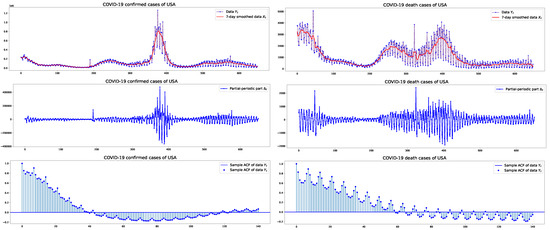
Figure 1. USA: COVID-19 daily confirmed/death cases $Y_t$ with their 7-day smoothed data $X_t$ and PPO part ${\Delta }_t=Y_t-X_t$ of size $n=651$ between 1 January 2021 and 13 October 2022, and the sample autocorrelation functions.

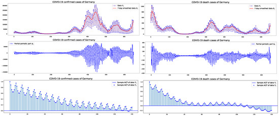
Figure 2. Germany: COVID-19 daily confirmed/death cases $Y_t$ with their 7-day smoothed data $X_t$ and PPO part ${\Delta }_t=Y_t-X_t$ of size $n=651$ between 1 January 2021 and 13 October 2022, and the sample autocorrelation functions.

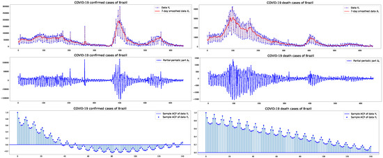
Figure 3. Brazil: COVID-19 daily confirmed/death cases $Y_t$ with their 7-day smoothed data $X_t$ and PPO part ${\Delta }_t=Y_t-X_t$ of size $n=651$ between 1 January 2021 and 13 October 2022, and the sample autocorrelation functions.

3.1. Estimation Results

The parameters of the model are estimated from the standardized data, as mentioned before. For the PPO-ARIMA model $Y_t=X_t+{\Delta }_t+{\epsilon }_t$, the 7-day smoothed moving averaging data $X_t$ are fitted to an ARIMA model. To do this, we test the unit–root non-stationarity of $X_t$ by means of the ADF (augmented Dickey–Fuller) test. In Table 2, the results of the ADF test on the data $\left\{X_t\right\}$ are reported along with the p-values. The death cases of the USA and the confirmed cases in Brazil are 0.0019 and 0.0016, respectively, as the p-values of the ADF test. Since the values are less than 0.01, we reject the unit–root non-stationarity at the 1% level. Thus, they have order $d=0$ in the fitted ARIMA ($p,d,q$) models. Other orders are selected by the criteria, such as AIC and root mean square errors. Table 2 also presents orders of the ARIMA ($p,d,q$) models $\left\{X_t\right\}$ as well as coefficient estimates and their standard error (s.e).

Table 2. Results of the ADF test, orders of the ARIMA $(p, d, q)$ model, coefficient estimates ${\widehat{\varphi }}_1,{\widehat{\theta }}_1,{\widehat{\theta }}_2$, and the standard error (s.e.) of the ARIMA part $X_t$ in the PPO-ARIMA model $Y_t=$$X_t+$${\Delta }_t+{\epsilon }_t$, where $Y_t$ denotes the (standardized) COVID-19 confirmed (C)/death (D) case data from the USA, Germany, and Brazil, with $n=651$ days between 1 January 2021 and 13 October 2022.

	USA		Germany		Brazil
	C	D	C	D	C	D
Test statistics	−2.7255	−3.9143 ${}^{†}$	−1.6715	−2.5841	−3.967 ${}^{†}$	−1.8058
p-value	0.0697	0.0019 ${}^{†}$	0.4458	0.0963	0.0016 ${}^{†}$	0.3776
orders ($p,d,q)$	(1,1,2)	(1,0,1)	(1.1.1)	(1,1,2)	(1,0,2)	(1,1,2)
${\widehat{\varphi }}_1$	0.9562	0.9986	0.4115	0.9621	0.9913	0.9499
	(0.005)	(0.004)	(0.028)	(0.005)	(0.003)	(0.017)
${\widehat{\theta }}_1$	−0.7722	0.2703	0.4279	−0.4833	0.1981	−0.6314
	(0.014)	(0.025)	(0.025)	(0.016)	(0.019)	(0.029)
${\widehat{\theta }}_2$	0.2012	-	-	−0.1788	0.2308	−0.1951
	(0.021)	-	-	(0.016)	(0.027)	(0.022)

${}^{†}$ indicates that the ADF test rejects the unit–root non-stationarity at a 1% level.

Table 3 presents the estimates of parameters of the PPO part $\left\{{\Delta }_t\right\}$: Threshold $x_0$ is selected as the minimum of $\left\{X_t\right\}$. This is because all observations appear to be oscillated, even though some small magnitudes yield slight fluctuations, as seen in Figure 1, Figure 2 and Figure 3. However, unless all observations are oscillated, one method for choosing $x_0$ is to minimize the mean square error. In other words, we choose ${\widehat{x}}_0=argminMSE\left(x_0\right)$, where $MSE\left(x_0\right)=\frac{1}{n}{\sum }_{t=1}^n{\widehat{ϵ}}_t^2$, the mean square error. ${\widehat{ϵ}}_t=Y_t-{\widehat{X}}_t-{\widehat{\Delta }}_t$, ${\widehat{X}}_t$ is the fitted value derived from the coefficient estimates of the ARIMA part, and ${\widehat{\Delta }}_t$ is the fitted value derived from the estimates ${\widehat{\omega }}_{\ell }$ and $\widehat{\delta }$. In this work, we use the minimum of $\left\{X_t\right\}$ for the value of $x_0$, because all plots of the second rows of Figure 1, Figure 2 and Figure 3 show the oscillations.

Table 3. Estimation results of parameters for the partial-periodic part ${\Delta }_t$ in the PPO-ARIMA model $Y_t=X_t+{\Delta }_t+{\epsilon }_t$, where $Y_t$ is the (standardized) COVID-19 confirmed (C)/death (D) case data from the USA, Germany, and Brazil, with $n=651$ days between 1 January 2021 and 13 October 2022.

	USA		Germany		Brazil
	C	D	C	D	C	D
$x_0$	−0.7295	−1.063	−0.7795	−0.9788	−1.0506	−0.8798
$\delta$	1.02	1.358	1.13	0.956	0.90	0.794
${\omega }_0$	0.2486	0.3020	0.2609	0.1287	0.2661	0.2453
${\omega }_1$	0.2113	0.1514	0.1188	0.0492	0.2660	0.2314
${\omega }_2$	0.2399	0.3126	−0.3643	−0.3501	0.1948	0.1355
${\omega }_3$	−0.3816	−0.3443	−0.7460	−0.5727	−0.0373	−0.0437
${\omega }_4$	−0.5119	−0.4915	−0.1698	0.1421	−0.4992	−0.4823
${\omega }_5$	−0.0525	−0.2193	0.4784	0.3045	−0.4243	−0.4141
${\omega }_6$	0.1104	0.3235	0.4415	0.2448	0.1542	0.2450

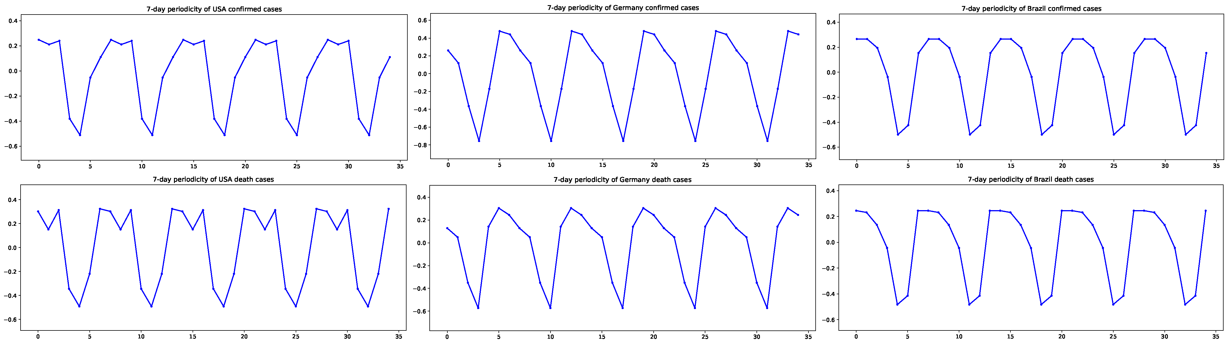
The exponent $\delta$ and the weights ${\omega }_{\ell }$ are estimated by means of arguments stated in Section 2.2. The values of the estimated weights in Table 3 indicate oscillations. In particular, in the confirmed case of Germany, stronger oscillations occur, which can be seen in the plot of the PPO part $\left\{{\Delta }_t\right\}$ in the second row and second column of Figure 2. To highlight clear oscillations, Figure 4 depicts the periodicity of the estimates of weights, ${\widehat{\omega }}_{\ell }$, $\ell \in \{0, 1, \dots ,6\}$. In the figure, weights are repeatedly plotted so that the 7-day periodicity can be seen. Note that 0 on the horizontal axis indicates Friday. In the USA and Brazil, on Friday, there are more confirmed/death cases than on other days, whereas in Germany, Wednesdays see a higher number of cases than on other days.

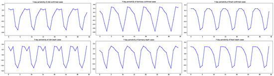
Figure 4. The 7-day periodicity of the confirmed and death cases in the USA, Germany, and Brazil: (Repetition of $\{{\omega }_0,{\omega }_1, \dots ,{\omega }_6\}$; 0 = Friday on the horizontal axis.

3.2. Prediction Results

Now, in order to see the forecasting performance, an out-of-sample forecasting analysis is conducted. We first compute k-step ahead predicted values, ($k=1, 2, \dots$), along with their accuracy measures, and secondly construct 95% prediction intervals of one-step ahead forecasts. For the out-of-sample forecasting, the total sample is divided into two subsamples. As the sample size is $T=651$, the initial in-sample of size $n=231$ and out-of-sample of size $m=420$ are split into two subsamples. A rolling window technique is used to compute k-step ahead forecasts and their errors. At time t, the k-step ahead forecast of $Y_t$ is given by

$${\widehat{Y}}_t\left(k\right)={\widehat{X}}_{t+k}+{\widehat{\omega }}_{{\ell }_k}{\left|{\widehat{X}}_{t+k}-{\widehat{x}}_0\right|}^{\widehat{\delta }}{\mathbb{I}}_{\{{\widehat{X}}_{t+k}>{\widehat{x}}_0\}}$$

where ${\widehat{X}}_{t+k}$ is the k-step ahead forecast of $X_t$ by using the ARIMA model and ${\ell }_k=t+k$ mod $\tau$.

From these, the root mean square error (RMSE), the mean absolute error (MAE), and heterogeneous MAE (HMAE) of the k-step ahead forecasts are evaluated as follows:

$$RMS{E}_k={\left(\frac{1}{m}\sum _{i=1}^m{(Y_{t_i+k}-{\widehat{Y}}_{t_i}\left(k\right))}^2\right)}^{1/2}$$

$$MA{E}_k=\frac{1}{m}\sum _{i=1}^m|Y_{t_i+k}-{\widehat{Y}}_{t_i}\left(k\right)|$$

$$HMA{E}_k=\frac{1}{m}\sum _{i=1}^m\left|\frac{Y_{t_i+k}^o-{\widehat{Y}}_{t_i}^o\left(k\right)}{Y_{t_i+k}^o}\right|$$

where $Y_t$ and $Y_t^o$ are standardized and unstandardized data, respectively. Because $\left\{Y_t\right\}$ and $\left\{{\widehat{Y}}_t\right\}$ are standardized data and their forecasts, respectively, RMSE and MAE are appropriate metrics to compare all confirmed and death case data, along with those of other existing models, such as ARIMA and SARIMA models. Also, in the expression of HMAE, the denominators are unstandardized since it is important to see the ratio of the forecast errors to the positive original data, and if the standardized data are used in the HMAE, the denominator can be too small in absolute terms, nearly zero, which would lead to too big HMAE values, rendering them nonsensical. All six instances of confirmed and death cases in the three countries are compared with each other, together with those from the other two models; thus, the formulas of the three error metrics using $Y_t$ in RMSE, MAE, and $Y_t^o$ in HMAE are appropriate.

The three accuracy measures in Table 4 are obtained by the formulas above with $m=420$ and $k\in \{1, 2, 3\}$. Also, Table 4 reports comparisons with the existing models: the ARIMA and SARIMA models. Model selections for the ARIMA ($p, d, q$) models are given by the criteria of the best AIC values via Python auto_arima, setting the range of orders: $p,q\in \{0, 1, \dots , 7\}$ and $d\in \{0, 1, 2\}$. In the SARIMA models, seasonal period $s = 7$ is taken and order is chosen by the AIC values as well. In Table 4, we see that the PPO-ARIMA models have the smallest error values in most cases, except for the HMAE on the one-step ahead forecasts of the USA and two-, three-steps of Germany. The best values are indicated by the bolded numbers in Table 4. Most of the values of RMSE, MAE, and HMAE in Table 4 are the best in the PPO-ARIMA models. In Germany’s COVID-19 data, instead of the PPO-ARIMA model, the ARIMA model gives the best values of HMAE for the two- and three-step ahead forecasts. It might be due to relatively large values of real data in the last part of the sample, as seen in Figure 2.

Table 4. Out-of-sample forecasting results and comparison: RMSE, MAE, and HMAE of k-step ahead forecasts, ($k=1, 2, 3$), for the last 420 days in the PPO-ARIMA models for the COVID-19 confirmed (C)/death (D) case data from the USA, Germany, and Brazil, and a comparison with those of the ARIMA and SARIMA models.

			USA		Germany		Brazil
		$\mathit{k}$-Step	C	D	C	D	C	D
RMSE	ARIMA	1	0.3335	0.3901	0.2457	0.2185	0.4915	0.1436
		2	0.6597	0.6155	0.6118	0.4143	0.6432	0.2039
		3	0.7821	0.8225	0.9098	0.5764	0.8162	0.2624
	SARIMA	1	0.3086	0.4115	0.2520	0.2155	0.4985	0.1635
		2	0.6947	0.7014	0.6262	0.4331	0.6388	0.2259
		3	0.8171	0.9384	0.9251	0.5977	0.8281	0.2832
	PPO-ARIMA	1	0.3153	0.2920	0.2027	0.1669	0.3152	0.0989
		2	0.4901	0.5348	0.4648	0.3419	0.5001	0.1865
		3	0.5306	0.7867	0.8325	0.5358	0.5857	0.1926
MAE	ARIMA	1	0.1729	0.2307	0.1446	0.1413	0.2609	0.0940
		2	0.3397	0.4184	0.4093	0.2919	0.3772	0.1376
		3	0.4578	0.6014	0.6365	0.4340	0.4888	0.1834
	SARIMA	1	0.1571	0.2361	0.1459	0.1441	0.2813	0.1031
		2	0.3521	0.4722	0.4164	0.3048	0.3837	0.1527
		3	0.4817	0.6895	0.6485	0.4453	0.5107	0.1976
	PPO-ARIMA	1	0.1615	0.1994	0.1287	0.1077	0.1650	0.0614
		2	0.2672	0.3691	0.3008	0.2339	0.2670	0.1119
		3	0.3133	0.5509	0.5599	0.3931	0.3207	0.1355
HMAE	ARIMA	1	0.2327	0.3421	0.2038	0.2526	0.4161	0.4318
		2	0.5237	0.7645	0.5549	0.4798	0.6921	0.7285
		3	0.8004	1.2584	0.9726	0.7974	0.9736	0.9928
	SARIMA	1	0.2081	0.3805	0.2063	0.2817	0.5245	0.4542
		2	0.5375	0.9115	0.5753	0.5315	0.7613	0.8382
		3	0.8292	1.5192	1.0082	0.8297	1.0043	1.0679
	PPO-ARIMA	1	0.2330	0.3998	0.2008	0.2157	0.3463	0.2946
		2	0.4450	0.7436	0.6071	0.5271	0.4756	0.5286
		3	0.5961	1.2010	1.1289	0.9019	0.6949	0.8046

The bold indicates the best values.

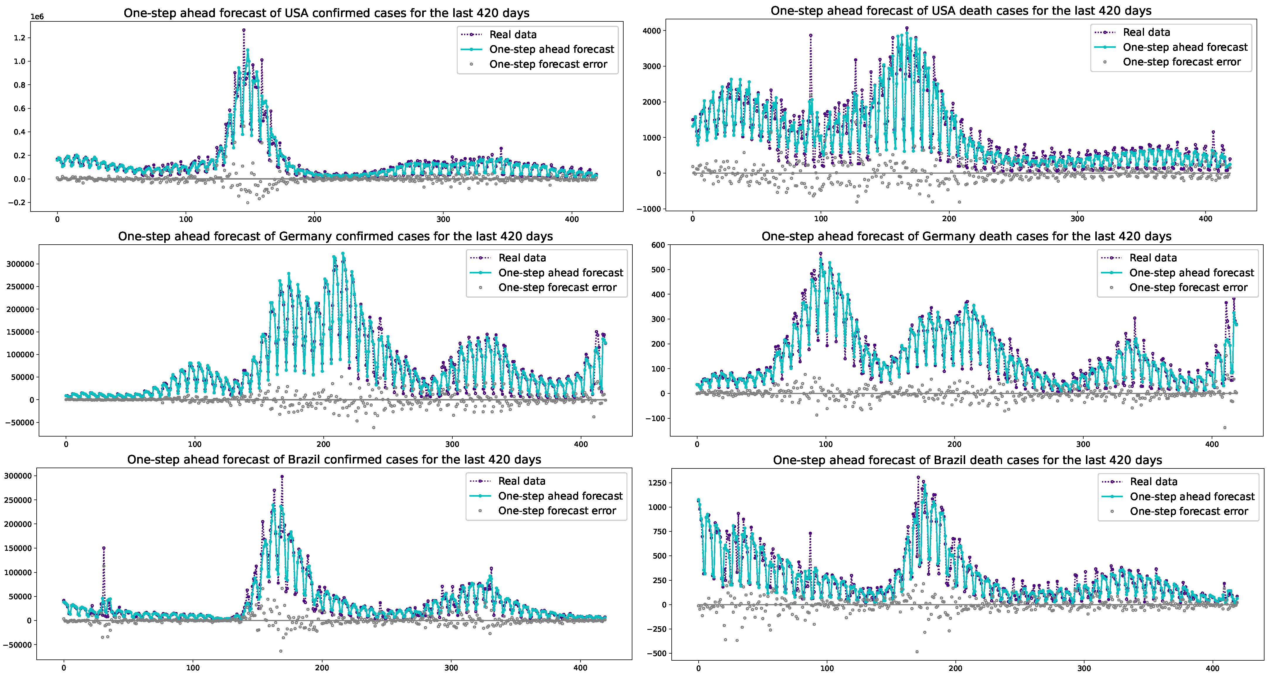
The one-step ahead forecasts by the PPO-ARIMA models for the last 420 days and their errors in the USA, Germany, and Brazil, are depicted, respectively, in Figure 5. The one-step ahead forecasted values fit well with the actual data, even though there are some errors. Also, we see that periodic oscillations of one-step ahead forecasts seem to be as strong as the actual data.

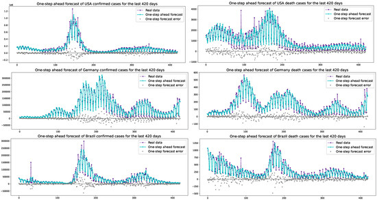
Figure 5. One-step ahead forecasts of COVID-19 confirmed/death cases and one-step forecast errors for the last 420 days in the USA, Germany, and Brazil.

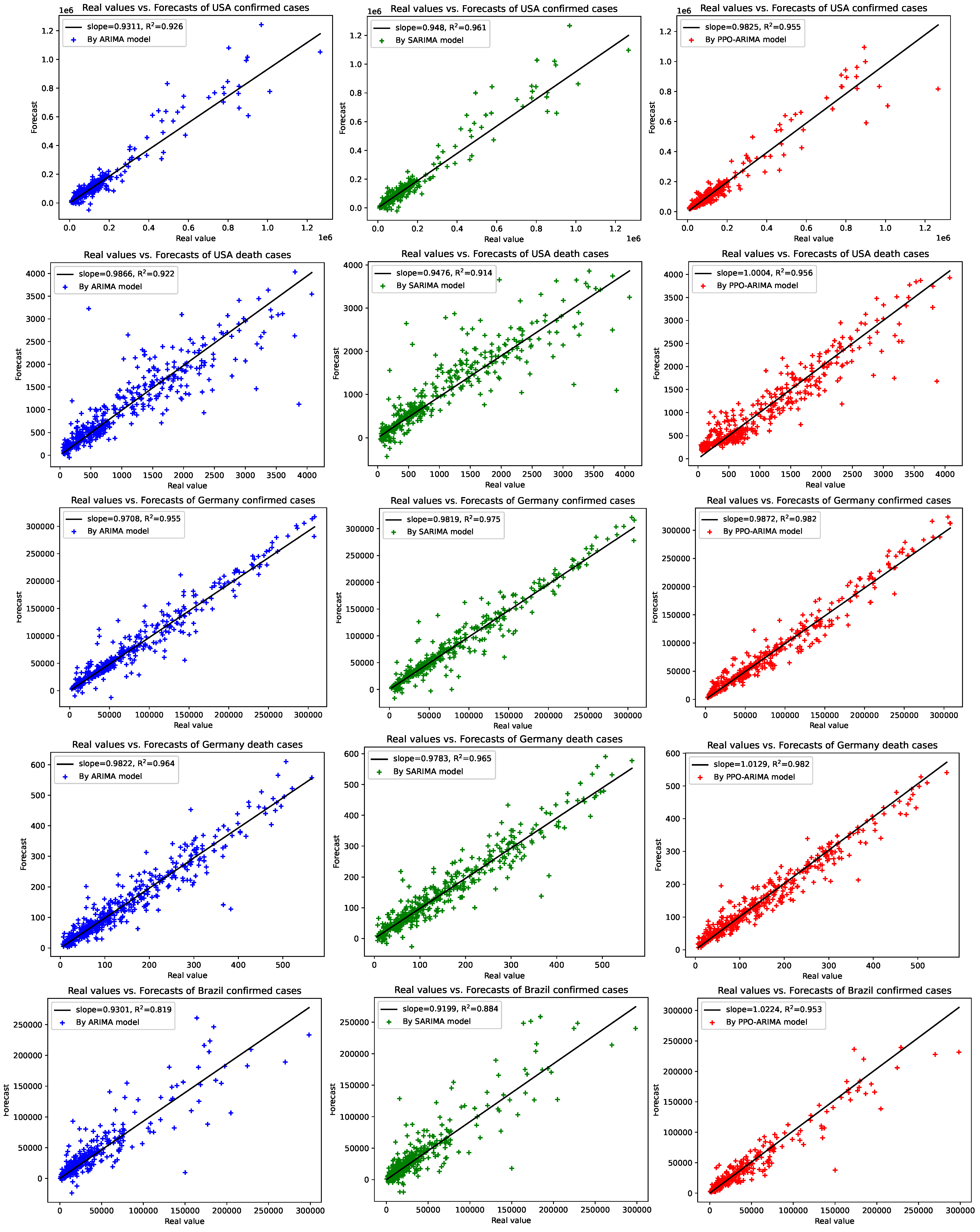
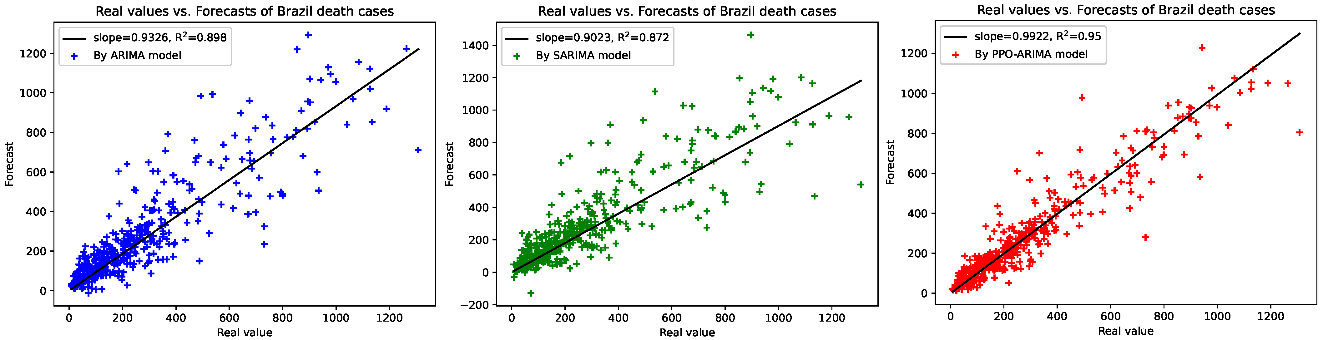
To understand how well the PPO-ARIMA model performs in prediction errors, compared to other models, we provide two results: illustrations between real values and forecasts, and efficiency evaluations. First, Figure 6 shows a straight-line relationship between real values and forecasts, along with slopes and $R^2$-values of the linear regressions in the three models. In the PPO-ARIMA models, slopes are closer to one and $R^2$-values are higher than the other two models. As the second measure, the efficiency of the prediction by the PPO-ARIMA model is evaluated from the error values in Table 4. For an error function $f\in \{RMSE, MAE, HMAE\}$, the efficiencies denoted by Effi${}_A$ and Effi${}_S$, relative to the two benchmarks, the ARIMA and SARIMA models, are defined by

$${\mathrm{Effi}}_A=100\times \left(\frac{f_A-f_{PPO}}{f_{PPO}}\right),{\mathrm{Effi}}_S=100\times \left(\frac{f_S-f_{PPO}}{f_{PPO}}\right)$$

where A on the subscript stands for ARIMA, S for SARIMA, and $PPO$ for the PPO-ARIMA model. The results of the PPO-ARIMA prediction efficiencies, Effi${}_A$ and Effi${}_S$, relative to the ARIMA and SARIMA models, are reported in Table 5. Because the SARIMA model is a full periodic oscillation model, SARIMA underperforms compared to the ARIMA model and, thus, efficiency relative to the SARIMA model is better than that of the ARIMA model. Note that the ARIMA models use order $p=7$ in their AR parts, chosen by the criteria of the best AIC values. Since the data do not have full periodic oscillation, the comparison with the SARIMA model might be somewhat unfair. To solve the unfairness, an action, such as the regime-switching Markov chain, might be required in the SARIMA model. However, this would require extensive theoretical and empirical analysis and is therefore left for future study.

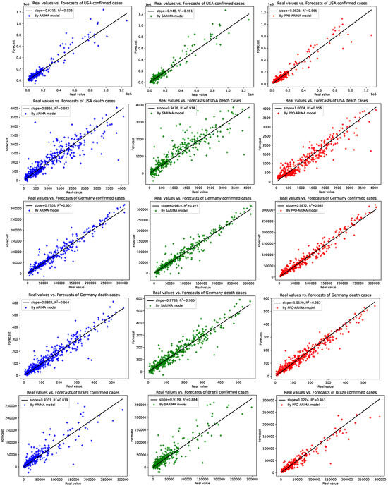
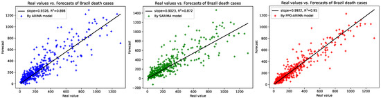
Figure 6. Real values vs. forecasted values by ARIMA, SARIMA, and PPO-ARIMA models for the confirmed/death cases in the USA, Germany, and Brazil: Each plot gives slopes and $R^2$-values of linear regressions.

Table 5. Efficiency(%) of prediction by the PPO-ARIMA model, relative to the ARIMA and SARIMA models, respectively, defined as Effi${}_A=100\times (f_A-f_{PPO})/f_{PPO}$ and Effi${}_S=100\times (f_S-f_{PPO})/f_{PPO}$ where $f\in \{RMSE,MAE,HMAE\}$; A = ARIMA, S = SARIMA, and PPO = PPO-ARIMA model.

			USA		Germany		Brazil
$\mathit{f}$	$\mathit{k}$-Step		C	D	C	D	C	D
RMSE	Effi${}_A$	1	5.80	33.59	21.21	30.92	55.93	45.19
		2	34.61	15.09	31.63	21.18	28.61	9.33
		3	47.40	4.55	9.29	7.57	39.35	36.24
	Effi${}_S$	1	−2.12	40.92	24.32	29.12	58.15	65.32
		2	41.75	32.15	34.72	26.67	27.72	21.17
		3	53.99	19.18	42.65	11.55	41.37	47.04
MAE	Effi${}_A$	1	7.06	15.69	12.35	31.20	58.12	53.09
		2	27.13	13.36	36.07	23.79	41.27	22.96
		3	46.12	9.17	13.68	10.40	52.41	35.35
	Effi${}_S$	1	−2.72	18.41	13.36	33.79	70.48	67.92
		2	31.77	27.93	38.43	30.31	43.71	36.46
		3	53.75	25.16	15.82	13.28	59.25	45.83
HMAE	Effi${}_A$	1	−0.13	−14.32	1.49	17.11	20.16	46.57
		2	17.68	2.81	−8.59	−8.97	45.52	37.82
		3	34.27	4.78	−13.84	−11.59	40.11	23.39
	Effi${}_S$	1	−10.68	−4.82	2.73	30.59	51.45	54.18
		2	20.78	22.58	−5.23	0.84	60.09	58.56
		3	30.10	26.49	−10.69	−8.01	44.52	32.72

From the efficiency results in Table 5, we conclude that our proposed PPO-ARIMA model improves the forecast errors, such as the RMSE, MAE, and HMAE for one-, two-, and three-step ahead forecasts. The superiority of the proposed model is demonstrated by large values of efficiency in Table 5. A maximum of 46–58% efficiency relative to the ARIMA model and 65–70% relative to the SARIMA model are seen in the error metrics of RMSE, MAE, and HMAE. Also, the PPO-ARIMA model achieves a maximum improvement of 55–65% in RMSE, 58–70% in MAE, and 46–60% in HMAE for the one-step forecasts, compared to the existing models.

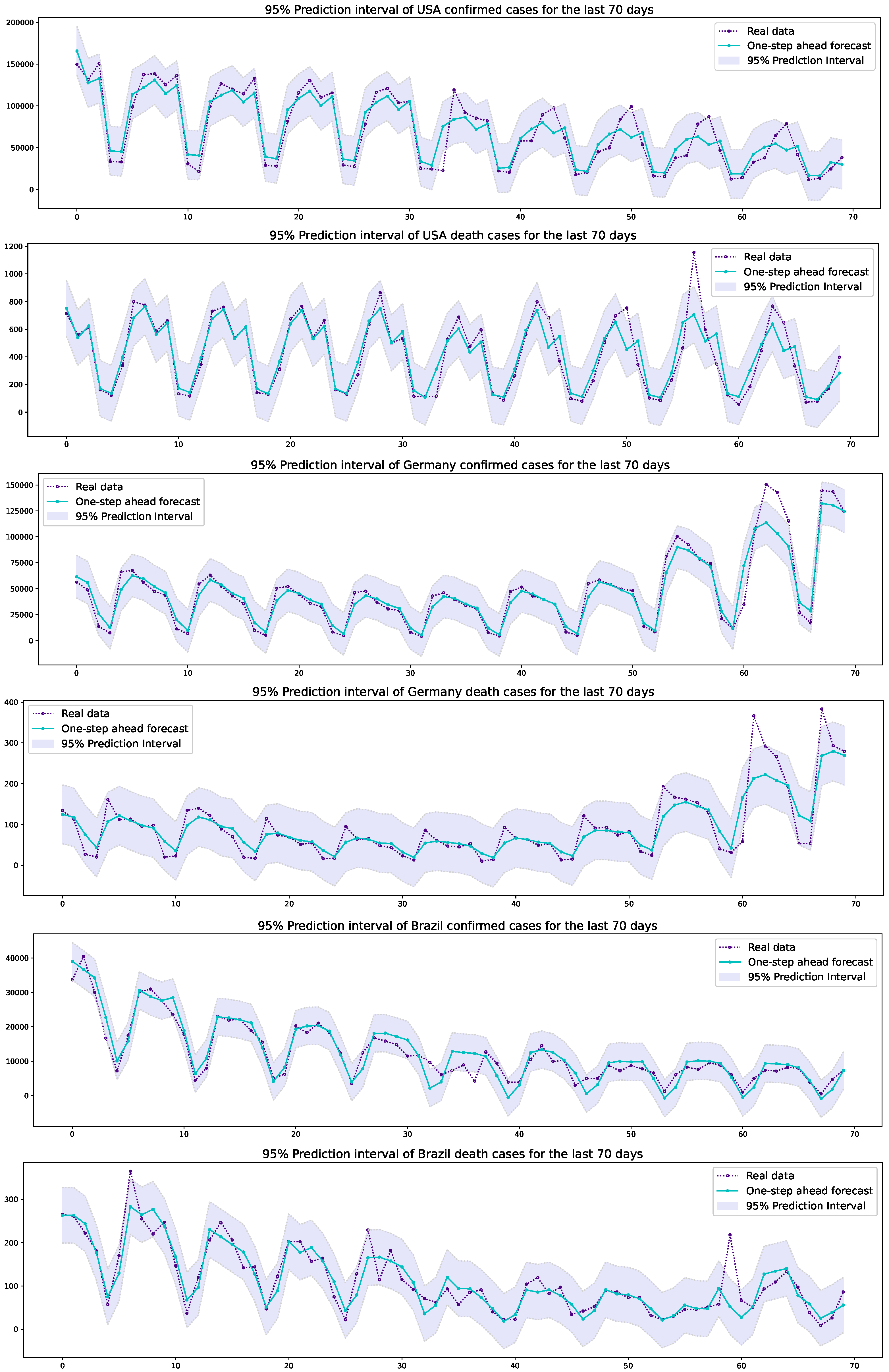
Finally, the 95% prediction intervals of the one-step forecasts are constructed by using a normal approximation. For the empirical analysis, among the 420 days forecasts in Figure 4, the last 70 days are selected to draw the prediction intervals, which are computed as follows:

$$\left[{\widehat{Y}}_t\left(1\right)-z_{0.975}{\widehat{\sigma }}_1,{\widehat{Y}}_t\left(1\right)+z_{0.975}{\widehat{\sigma }}_1\right]$$

(5)

where $z_{0.975}=1.96$ is used and ${\widehat{\sigma }}_1^2$ is the one-step prediction variance given by ${\widehat{\sigma }}_1^2=\frac{1}{70}{\sum }_{i=1}^{70}{(Y_{t_i+1}-{\widehat{Y}}_{t_i}\left(1\right))}^2-{\left(\frac{1}{70}{\sum }_{i=1}^{70}(Y_{t_i+1}-{\widehat{Y}}_{t_i}\left(1\right))\right)}^2.$ The 95% prediction intervals for the last 70 days are illustrated in Figure 7. Most of the actual data belong to the prediction intervals; indeed, the 95% prediction intervals include 94.28–98.57% of actual data. These values are close to the nominal coverage of 95%. The reason for the deviation between the nominal and empirical coverage is that the sample size is 70 in the construction of the intervals and the evaluation of the prediction variance. It is well-known that the empirical coverage converges to the nominal one as the size increases. Also, we see from Figure 7 that the prediction intervals possess the features of oscillations with a periodicity of 7 as well. The prediction intervals in (5) have the same length, $2z_{0.975}{\widehat{\sigma }}_1$, and the oscillations occur, depending on the values of the one-step predicted values. In the cases of Germany, the last ten days have somewhat large extreme actual values in both confirmed and death cases (see Figure 7) and, thus, because of the large extremes, the proposed model for the cases of Germany does not give the best values in the HMAE for the two- and three-step ahead forecasts in Table 4. However, the 95% prediction intervals need to be improved because the residuals might not follow the normal distribution. As for the prediction interval improvements, Ref. [28] discussed the bootstrap improvement on the prediction intervals for COVID-19 data, along with the approach of the Laplace distribution. For the PPO-ARIMA model and its prediction in this work, the topic of prediction interval improvement will be deferred to further study.

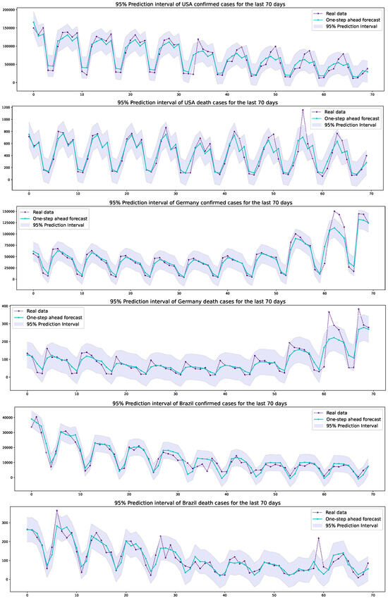
Figure 7. The 95% prediction intervals of the USA, Germany, and Brazil confirmed/death cases for the last 70 days.

As discussed above in Section 2, the roles of threshold $x_0$ and exponent $\delta$ are important because they might incur problems of overfitting or underfitting. Even though $x_0$ is chosen as the minimum of the standardized data in this work, for other real-world data, some other criteria should be chosen, for instance, through MSE, as discussed in Section 3.1. As seen in the plots of weights ${\omega }_{\ell }$, $\ell \in \{0, 1, \dots ,\tau -1\}$, in Figure 4, which shows the 7-day periodicity of COVID-19 data, most have distinct periodic oscillations with large amplitudes. However, in other datasets with somewhat small amplitudes of oscillations, we need to perform more actions like finding the standard error of the estimates, which are not given in this work. Instead of the consistency of the estimators, the asymptotic distributions should be established to find the standard errors. This generalizability problem addresses potential concerns and will be dealt with in a future study.

4. Discussion and Conclusions

The scientific community should continue to make efforts to predict and mitigate the COVID-19 pandemic using reliable scientific methods as long as the virus continues to spread globally. In particular, as discussed by [20], the high-frequency oscillatory patterns in COVID-19 infections and deaths should be incorporated into prediction analyses for a comprehensive understanding and improved forecasting. A remarkable feature, resulting from testing bias or human behaviors in health systems, is the periodic oscillations observed in the most affected countries and continents, such as North America and Europe. As [22,23] noted, identifying such cyclical oscillations in COVID-19 time series data is a significant issue. Reliable forecasting of these oscillation phenomena will mark a notable advancement in the history of the COVID-19 pandemic.

This study focused on forecasting COVID-19 data with 7-day cyclical fluctuations by combining the ARIMA model with a partial periodic oscillation model. Employing this proposed predictive model, which utilizes a straightforward mathematical approach, we predicted confirmed and death cases of COVID-19. The USA, Germany, and Brazil were selected for empirical analysis due to the strong oscillatory patterns in their COVID-19 data. New daily COVID-19 data for both confirmed and death cases in these three countries were empirically estimated. Out-of-sample forecasting experiments were conducted to evaluate prediction accuracy and construct 95% prediction intervals.

In order to see the forecasting performance, prediction accuracy measures, such as root mean square error (RMSE), mean absolute error (MAE), and heterogeneous MAE (HMAE), were evaluated. RMSE, MAE, and HMAE of the one-, two-, and three-step ahead forecasts of COVID-19 confirmed/death cases were computed and compared with other existing models. Comparisons with ARIMA models (with order $p=7$ of the AR part) and SARIMA models (with 7-day periodicity) were reported; model selections were determined by the optimal AIC values. The efficiencies of the PPO-ARIMA model, relative to each of the two benchmarks, were evaluated. The results showed that our model improved the ARIMA model by a maximum of 58% and the SARIMA model by 70%. More specifically, predictions of the daily COVID-19 cases can be improved by the PPO-ARIMA model: by a maximum of 55–65% in RMSE, 58–70% in MAE, and 46–60% in HMAE, compared to the existing models.

Moreover, the 95% prediction intervals of one-step ahead forecasts were constructed for the six cases; their illustrations showed that the intervals include 94.28–98.57% of actual data in the out-of-sample forecasting as well as exhibit interval–oscillation patterns, coincidentally.

The PPO-ARIMA model will be a practical tool for predicting the spread of the global COVID-19 pandemic. The results of this study can assist health institutions in medical resource allocation and emergency strategy development by providing more accurate statistical information. Hence, a contribution of this study is the identification and superior forecasting of partially weekly oscillating COVID-19 cases using the proposed model, coupled with a new mathematical approach. The PPO-ARIMA model is well-suited for data exhibiting partial oscillation, where the SARIMA model may not be appropriate. Also, our model can deliver robust results for fully oscillated data, for which the SARIMA model is suitable. This is because the values of the PPO part are proportional to the values of the ARIMA part. Therefore, the PPO-ARIMA model can offer optimal performance on data with periodicity and seasonality, whether it exhibits partial or full oscillation.

A limitation of this study is the residual analysis, from which the prediction intervals were constructed. Because this work focuses on the partial periodicity of COVID-19 data, the main concentration of the paper is not on the residual analysis. A complement to this would be the more refined construction of prediction intervals through the estimation of the distribution of residuals. This topic will be addressed in future work. Moreover, another limitation of this study is that it analyzed only three countries that have the strongest oscillations in the world. The PPO-ARIMA model could be applied to datasets from other countries with weaker oscillations. Experiments on more general datasets are needed to justify the robustness of the model.

A recent study about the exponential decay model by [11] showed its effectiveness for short-term forecasting. Our model also shows good performance in short-term forecasting by reflecting the 7-day periodicity. However, the approaches of the exponential decay model and the PPO-ARIMA model differ: the latter emphasizes oscillation, which is a critical aspect of our study. Their explicit comparison will be interesting and will need extensive experiments; therefore, it remains a topic for future study.

Three directions for further study related to the partial periodic oscillations of COVID-19 are suggested: First, in terms of time series modeling, other models such as a heterogeneous autoregression (HAR) model or nonparametric models could be adopted instead of the ARIMA model. As discussed by [28], the HAR model with lagged average regressors is suitable for the smoothed data of COVID-19, and thus, a combined model incorporating the HAR model with partial periodic oscillations might offer enhanced predictive ability. Second, some exogenous variables can be added as significant regressors in the model, as in [30]. For example, the booster vaccination rate, which influences the spread of COVID-19, could be added as an explanatory variable. Third, from the perspective of forecast error distribution, efforts to minimize errors could be made through distribution inferences. This work assumed normal approximation for the residuals to construct prediction intervals. However, for a refinement of more accurate prediction intervals, the residual distribution can be inferred by means of the bootstrap procedure or kernel method. A comparative analysis of various prediction intervals, by evaluating their average length, empirical coverage probability, and mean interval score, will be able to yield the most improved prediction for the oscillatory patterns of COVID-19, which remains an area for future research. Overall, a variety of statistical extensions will be attempted in data analysis for COVID-19 prediction. This could be a contributing role of statistics in fostering a healthy society, by providing insights into disease transmission through modeling and forecasting with reduced errors.

References

- Ribeiro, M.H.D.M.; Silva, R.G.D.; Mariani, V.C.; Coelho, L.D.S. Short-term forecasting COVID-19 cumulative confirmed cases: Perspectives for Brazil. Chaos Solitons Fractals 2020, 135, 109853. [Google Scholar] [CrossRef] [PubMed]
- Maleki, M.; Mahmoudi, M.; Wraith, D.; Pho, K. Time series modelling to fore cast the confirmed and recovered cases of COVID-19. Travel. Med. Infect. Dis. 2020, 37, 101742. [Google Scholar] [CrossRef] [PubMed]
- Maleki, M.; Mahmoudi, M.R.; Heydari, M.H. Modeling and forecasting the spread and death rate of coronavirus (COVID-19) in the world using time series models. Chaos Solitons Fractals 2020, 140, 110151. [Google Scholar] [CrossRef] [PubMed]
- Sarkar, K.; Khajanchi, S.; Nieto, J.J. Modeling and forecasting the COVID-19 pandemic in India. Chaos Solitons Fractals 2020, 139, 110049. [Google Scholar] [CrossRef] [PubMed]
- Balli, S. Data analysis of COVID-19 pandemic and short-term cumulative case forecasting using machine learning time series methods. Chaos Solitons Fractals 2021, 142, 110512. [Google Scholar] [CrossRef] [PubMed]
- Ala’raj, M.; Majdalawieh, M.; Nizamuddin, N. Modeling and forecasting of COVID-19 using a hybrid dynamic model based on SEIRD with ARIMA corrections. Infect. Dis. Model. 2021, 6, 98–111. [Google Scholar] [CrossRef]
- Kumar, Y.; Koul, A.; Kaur, S.; Hu, Y.C. Machine learning and deep learning based time series prediction and forecasting of ten nations’ COVID-19 pandemic. SN Comput. Sci. 2022, 4, 91. [Google Scholar] [CrossRef] [PubMed]
- Fang, L.; Wang, D.; Pan, G. Analysis and estimation of COVID-19 spreading in Russia based on ARIMA model. Sn Compr. Clin. Med. 2020, 2, 2521–2527. [Google Scholar] [CrossRef]
- Ilie, O.D.; Cojocariu, R.O.; Ciobica, A.; Timofte, S.I.; Mavroudis, I.; Doroftei, B. Fore casting the spreading of COVID-19 across Nine countries from Europe, Asia, and the American continents using the ARIMA Models. Microorganisms 2020, 8, 1158. [Google Scholar] [CrossRef]
- Toğa, G.; Atalay, B.; Toksari, M.D. COVID-19 prevalence forecasting using Autoregressive Integrated Moving Average (ARIMA) and Artifcial Neural Networks (ANN): Case of Turkey. J. Infect. Public Health 2021, 14, 811–816. [Google Scholar] [CrossRef]
- Bartolomeo, N.; Trerotoli, P.; Serio, G. Short-term forecast in the early stage of the COVID-19 outbreak in Italy. Application of a weighted and cumulative average daily growth rate to an exponential decay model. Infect. Dis. Model. 2021, 6, 212–221. [Google Scholar] [CrossRef] [PubMed]
- Petropoulos, F.; Makridakis, S.; Stylianou, N. COVID-19: Forecasting confirmed cases and deaths with a simple time series model. Int. J. Forecast. 2022, 38, 439–452. [Google Scholar] [CrossRef] [PubMed]
- Lourenco, J.; Recker, M. Natural, persistent oscillations in a spartial multi-strain disease system with application to dengue. PLoS Comput. Biol. 2013, 9, e1003308. [Google Scholar] [CrossRef] [PubMed]
- Selvaraj, P.; Wenger, E.A.; Gerardin, J. Seasonality and heterogeneity of malaria transmission determine success of interventions in high-endemic settings: A modeling study. BMC Infect. Dis. 2018, 18, 413. [Google Scholar] [CrossRef] [PubMed]
- Polwiang, S. The time series seasonal patterns of dengue fever and associated weather variables in Bangkok (2003–2017). BMC Infect. Dis. 2020, 20, 208. [Google Scholar] [CrossRef] [PubMed]
- Yuan, H.; Kramer, S.C.; Lau, E.H.Y.; Cowling, B.J.; Yang, W. Modeling influenza seasonality in the tropics and subtropics. PLoS Comput. Biol. 2021, 17, e1009050. [Google Scholar] [CrossRef] [PubMed]
- Li, Z.; Zhang, T. Analysis of a COVID-19 epidemic model with seasonality. Bull. Math. Biol. 2022, 84, 146. [Google Scholar] [CrossRef]
- Ndlovu, M.; Moyo, R.; Mpofu, M. Modelling COVID-19 infection with seasonality in Zimbabwe. Phys. Chem. Earth Parts A/B/C 2022, 127, 103167. [Google Scholar] [CrossRef]
- Wiemken, T.L.; Khan, F.; Puzniak, L.; Yang, W.; Simmering, J.; Polgreen, P.; Nguyen, J.L.; Jodar, L.; McLaughlin, J.M. Seasonal trends in COVID-19 cases, hospitalizations, and mortality in the United States and Europe. Sci. Rep. 2023, 13, 3886. [Google Scholar] [CrossRef]
- Bukhari, Q.; Jameel, Y.; Massaro, J.M.; D’Agostino, R.B.; Khan, S. Periodic oscillations in daily reported infections and deaths for coronavirus disease 2019. JAMA Netw. Open 2020, 3, e2017521. [Google Scholar] [CrossRef]
- Bergman, A.; Sella, Y.; Agre, P.; Casadevall, A. Oscillations in U.S. COVID-19 incidence and mortality data reflect diagnostic and reporting factors. mSystems 2020, 5, e00544-20. [Google Scholar] [CrossRef] [PubMed]
- Dehning, J.; Zierenberg, J.; Spitzner, F.P.; Wibral, M.; Neto, J.P.; Wilczek, M.; Priesmann, V. Inferring change points in the spread of COVID-19 reveals the effectiveness of interventions. Science 2020, 369, 160. [Google Scholar] [CrossRef] [PubMed]
- Huang, J.; Liu, X.; Zhang, L.; Zhao, Y.; Wang, D.; Gao, J.; Lian, X.; Liu, C. The oscillation-outbreak characteristic of the COVID-19 pandemic. Natl. Sci. Rev. 2021, 8, nwab100. [Google Scholar] [CrossRef] [PubMed]
- Soukhovolsky, V.; Kovalev, A.; Pitt, A.; Shulman, K.; Tarasova, O.; Kessel, B. The cyclicity of coronavirus cases: “Waves” and the “weekend effect”. Chaos Solitons Fractals 2021, 114, 110718. [Google Scholar] [CrossRef] [PubMed]
- Campi, G.; Bianconi, A. Periodic recurrent waves of Covid-19 epidemics and vaccination campaign. Chaos Solitons Fractals 2022, 160, 112216. [Google Scholar] [CrossRef] [PubMed]
- Simeonov, O.; Eaton, C.D. Modeling the drivers of oscillations in COVID-19 data on college campuses. Ann. Epidemiol. 2023, 82, 40–44. [Google Scholar] [CrossRef] [PubMed]
- Ekinci, A. Modeling and forecasting of growth rate of new COVID-19 cases in top nine affected countries: Considering conditional variance and asymmetric effect. Chaos Solitons Fractals 2021, 151, 111227. [Google Scholar] [CrossRef] [PubMed]
- Hwang, E. Prediction intervals of the COVID-19 cases by HAR models with growth rates and vaccination rates in top eight affected countries: Bootstrap improvement. Chaos Solitons Fractals 2022, 155, 111789. [Google Scholar] [CrossRef]
- Ceylan, Z. Estimation of COVID-19 prevalence in Italy, Spain and France. Sci. Total Environ. 2020, 729, 138817. [Google Scholar] [CrossRef]
- Selinger, C.; Choist, M.; Alison, S. Predicting COVID-19 incidence in French hospitals using human contact network analytics. Int. J. Infect. Dis. 2021, 111, 100–107. [Google Scholar] [CrossRef]
Disclaimer/Publisher’s Note: The statements, opinions and data contained in all publications are solely those of the individual author(s) and contributor(s) and not of MDPI and/or the editor(s). MDPI and/or the editor(s) disclaim responsibility for any injury to people or property resulting from any ideas, methods, instructions or products referred to in the content. |
© 2023 by the author. Licensee MDPI, Basel, Switzerland. This article is an open access article distributed under the terms and conditions of the Creative Commons Attribution (CC BY) license (https://creativecommons.org/licenses/by/4.0/).