On Non-Occurrence of the Inspection Paradox

Abstract

The well-known inspection paradox or waiting time paradox states that, in a renewal process, the inspection interval is stochastically larger than a common interarrival time having a distribution function F, where the inspection interval is given by the particular interarrival time containing the specified time point of process inspection. The inspection paradox may also be expressed in terms of expectations, where the order is strict, in general. A renewal process can be utilized to describe the arrivals of vehicles, customers, or claims, for example. As the inspection time may also be considered a random variable T with a left-continuous distribution function G independent of the renewal process, the question arises as to whether the inspection paradox inevitably occurs in this general situation, apart from in some marginal cases with respect to F and G. For a random inspection time T, it is seen that non-trivial choices lead to non-occurrence of the paradox. In this paper, a complete characterization of the non-occurrence of the inspection paradox is given with respect to G. Several examples and related assertions are shown, including the deterministic time situation.

1. Introduction

The inspection paradox, also known as the waiting time paradox or renewal paradox, describes a paradoxical effect where observing a running renewal process with events occurring at specific times leads to atypical findings, in the sense that the observed time interval between events may be longer than the other intervals. For example, this happens when the events in question are incoming claims of an insurance company and we arbitrarily select a time to observe the process (without knowledge of any claim arrival times). The time we select specifies an interval between two successive claims and we record the length of this time interval. It is stochastically larger than a regular (unobserved) interval between two successive incoming claims.

A renewal process can be used to model the times of incoming claims, where the waiting times between successive claims, called interarrival times, are modeled as realizations of independent and identically distributed non-negative random variables with cumulative distribution function F, for example. Thus, in a realized renewal process based on a non-degenerate distribution, we observe interarrival times of different lengths and, when inspecting the process at a certain time t, it will be very likely to observe a comparably larger time interval (cf. Feller [1], p. 13).

This paradoxical effect arises in various scenarios, such as waiting for a bus or a train (cf. Feller [1], p. 12–14, Masuda and Porter [2]), observing the lifetimes of identical batteries (cf. Ross [3], p. 460), in connection with sampling bias (cf. Stein and Dattero [4]), and in stochastic resetting (cf. Pal et al. [5]). In a medical context, Jenkins et al. [6] discussed how the perception of regularly occurring phase singularities, which are indicators for cardiac fibrillation, is influenced by the inspection paradox. They found that visual observation may systematically oversample phase singularities that last longer (potentially leading to errors) and that longer windows of observation can minimize the effect.

Much attention has been paid to the study of the inspection paradox, its properties, and implications (see, e.g., Gakis and Sivazlian [7], Angus [8], Ross [9]). In particular, considering a random variable for the time of inspection instead of a deterministic time leads to insights regarding the quantification of the effect (see, e.g., Kamps [10]). Herff et al. [11] derived an inequality for the length of the inspection interval with a random time and Rauwolf and Kamps [12] gave a general representation for the expected inspection interval length, which served as the basis for the main results in this work. Several explicit examples with random time and applications to earthquake and geyser data can be found in the literature (see, e.g., Liu and Peña [13], Rauwolf and Kamps [12]).

In the case of a deterministic inspection time t, the inspection paradox does not occur for a trivial choice of interarrival times having a degenerate distribution, i.e., for deterministic interval lengths. Moreover, it does not occur if the smallest possible interarrival time is larger than t; i.e., if the inspection is performed prior to the first event. However, for a random inspection time T with a left-continuous distribution function G, it is seen that there are examples with non-trivial choices of the distribution functions F and G where the paradox does not appear, meaning that the length of the inspection interval is also distributed as F.

In this general situation, we give a complete characterization of the non-occurrence of the inspection paradox with respect to the choice of G, as well as results for F in the classical case of degenerate G. The use of an additional random inspection time led to effects and a conclusion regarding the classical case with deterministic time, where non-occurrence of the paradoxical situations only happened for degenerate distributions.

In Section 2, we briefly recap the classical inspection paradox. Renewal processes with random time T are discussed in Section 3, along with examples. Section 4 contains a complete characterization of settings with respect to the distribution function G of T. A case with degenerate time t is studied in Section 5 regarding situations with non-occurrence of the inspection paradox leading to degenerate interarrival times.

2. The Classical Inspection Paradox Inequality

In order to formally introduce the inspection paradox, we first briefly recapitulate concepts of renewal processes. An introduction to renewal processes can be found in, e.g., Cox [14], Feller [1], Ross [3], Pinsky and Karlin [15], Mitov and Omey [16], and Kulkarni [17].

Let $X_1$, $X_2$, … be a sequence of non-negative, independent, and identically distributed (iid) random variables on some probability space with a common distribution function F, $F\left(0\right)<1$. These random variables will be called interarrival times in the following. Then, the sequence of occurrence times ${\left(S_n\right)}_{n\in {\mathbb{N}}_0}$ given by

$$S_0=0\mathrm{and}{S}_n=\sum _{i=1}^n{X}_i,n\in \mathbb{N},$$

defines a renewal process (see Figure 1). The corresponding renewal counting process is denoted by ${\left(N\left(t\right)\right)}_{t\ge 0}$, where

$$N\left(t\right):=\sum _{n=1}^{\infty }{\mathbb{1}}_{[0,t]}\left(S_n\right),t\ge 0,$$

counts the number of occurrences up to time t. In particular, $N\left(t\right)\ge n⟺S_n\le t$ holds for all $n\in {\mathbb{N}}_0$ and for all $t\ge 0$.

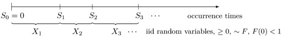
Figure 1. Renewal process.

When we inspect a renewal process at some fixed time $t>0$, exactly $N\left(t\right)$ renewals have already taken place. The last renewal prior to t was at time $S_{N\left(t\right)}$ and the subsequent renewal will occur at time $S_{N\left(t\right)+1}$. The renewal interval covering t is referred to as the “inspection interval” and its length is given by $X_{N\left(t\right)+1}=S_{N\left(t\right)+1}-S_{N\left(t\right)}$ (see Figure 2). Representations for the survival function and the expected value of the inspection interval length $X_{N\left(t\right)+1}$ can be found in the literature (see, e.g., Gakis and Sivazlian [7], pp. 44–45).

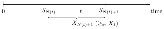
Figure 2. Inspection interval.

The inspection paradox of renewal theory then states that

$$P(X_{N\left(t\right)+1}>x)\ge P(X_1>x)\mathrm{for}\mathrm{all}x\ge 0\mathrm{and}t\ge 0$$

(1)

(cf. Angus [8], Ross [3]), which means that the inspection interval is stochastically larger than a common renewal interval, i.e., $X_{N\left(t\right)+1}{\ge }_{\mathrm{st}}{X}_1$. Consequently, in terms of expected values, the mean inspection interval length exceeds the mean length of any regular renewal interval, in the sense that

$$E{X}_{N\left(t\right)+1}\ge E{X}_1\mathrm{for}\mathrm{all}t\ge 0.$$

(2)

No paradoxical effect occurs in the trivial case where the interarrival times have a degenerate distribution, i.e., $X_i\sim {ϵ}_a$, $i\in \mathbb{N}$, for some $a>0$, as equality holds in the inspection paradox, i.e., $P(X_{N\left(t\right)+1}>x)={\mathbb{1}}_{(a,\infty ]}\left(x\right)=P(X_1>x)$ for all $x\ge 0$, and all events in the corresponding renewal process take place perfectly on time. In other words, all time intervals (including the inspected interval) have precisely the same length. Up to this point, it has remained open whether this is the only example in which equality holds for fixed t. The answer will be provided in the following sections by means of a generalization to a random inspection time T, for which the equality in (1) and (2) is characterized.

3. The Inspection Paradox with a Random Inspection Time

Instead of a fixed point in time $t\ge 0$, we can also consider a random variable to model the time of inspection. Let T be such a random inspection time, i.e., a non-negative random variable that is independent of the renewal process and has a left-continuous distribution function G given by $G\left(t\right)=P(T<t)$, $t\in \mathbb{R}$.

Then, (1) implies that the paradoxical effect occurs as in the classical inspection paradox with

$$P(X_{N\left(T\right)+1}>x)\ge P(X_1>x)\mathrm{for}\mathrm{all}x\ge 0,$$

(3)

i.e., $X_{N\left(T\right)+1}{\ge }_{\mathrm{st}}{X}_1$, and from (2) we conclude

$$E\left(X_{N\left(T\right)+1}\right)\ge E\left(X_1\right)$$

(4)

for the inspection paradox in terms of expectations.

In Section 2, we saw that equality in (1) in the fixed time case, i.e., for the choice $T\sim {ϵ}_t$, happens when the interarrival times have a degenerate distribution. The following example shows that, in a trivial case but for non-degenerate distributions of $X_1$ and T, equality in (3) and (4) holds true. Thus, introducing a random inspection time can lead to other cases with equality in (3) and (4).

Example 1.

Consider a Binomial renewal process with interarrival times having a geometric distribution on $\mathbb{N}$, i.e.,

$$P(X_i=k)=p{(1-p)}^{k-1},k\in \mathbb{N},i\in \mathbb{N},$$

and a random inspection time T with a two-point distribution, i.e., with $P(T=0)=P(T=1/2)=1/2$. Since $N\left(t\right)=0$ for $t<1$, we have $X_{N\left(t\right)+1}=X_1$, and thus $X_{N\left(T\right)+1}=X_1$ holds. The situation is trivial in the sense that the inspection is made prior to $X_1$. In particular, the distribution function G is constant on the support of the interarrival times with $G\left(k\right)=P(T<k)=1$ for all $k\in \mathbb{N}$.

On the other hand, in many well-known examples, Inequality (1) is strict for $t>0$ and so is (3); e.g., this is the case for a Poisson process with exponentially distributed interarrival times. The same holds true in connection with random inspection times; we refer to Liu and Peña [13] who discussed the choice of an exponentially distributed random inspection time.

In fact, the gap between the expected inspection interval length and a common expected interval length can be quantified for any choice of distribution. Rauwolf and Kamps [12] derived the following representation

$$E\phi \left(X_{N\left(T\right)+1}\right)=E\phi \left(X_1\right)+\sum _{n=1}^{\infty }\mathrm{Cov}(\phi \left(X_n\right),G\left(S_n\right)),$$

(5)

where $\phi :[0,\infty )\to [0,\infty )$ is a measurable function such that all expected values and integrals are well-defined and exist finitely. If $\phi$ is monotone non-decreasing, then all covariance terms are non-negative. In particular, this leads to a representation for the expected inspection interval length by choosing $\phi \left(x\right)=x$, $x\ge 0$,

$$E{X}_{N\left(T\right)+1}=E{X}_1+\sum _{n=1}^{\infty }\mathrm{Cov}(X_n,G\left(S_n\right)),$$

(6)

and to a representation for $P(X_{N\left(T\right)+1}>z)$ by choosing $\phi \left(x\right)={\mathbb{1}}_{(z,\infty )}\left(x\right)$, $x\ge 0$, $z\ge 0$. Thus, Inequalities (3) and (4) can be derived from (5), and choosing $T\sim {ϵ}_t$ leads to formulae in the classical case from Section 2.

As in Example 1, the introduction of a random inspection time T leads to various other possible and non-degenerate cases with non-occurrence of the inspection paradox. Concerning the identification of these respective situations, Formula (5) offers the option to examine cases where all covariance terms are equal to zero. On the other hand, Formula (5) also facilitates the study of situations with possible large gaps between $E{X}_{N\left(T\right)+1}$ and $E{X}_1$, say. For examples, we refer to [12].

In the following discussion, we will need the left and right endpoints of the support of the interarrival times, the formal introduction of which is given in Notation 1.

Notation 1.

Let X be a random variable with right-continuous distribution function F. Let $F^{-1}$ be the quantile function defined by $F^{-1}\left(y\right):=inf\{x:F\left(x\right)\ge y\}$, $y\in (0,1)$. Then, the left and right endpoints α and ω of the support of X are denoted by

$$\alpha :\mathrm{=}\underset{x\to 0^{+}}{lim}{F}^{-1}\left(x\right)\mathit{and}\omega :\mathrm{=}\underset{x\to 1^{-}}{lim}{F}^{-1}\left(x\right).$$

The support of X then lies in the interval $[\alpha ,\omega ]$ if $\omega <\infty$ or in $[\alpha ,\infty )$, otherwise, and will be denoted by $\mathrm{supp}\left(X\right)$.

The following result by Behboodian [18] given in Lemma 1 can be utilized to determine whether a covariance of two functions of a random variable is zero. In particular, this will be applied to determine whether the covariance terms in (5) are positive or zero. An alternative proof can be found in Rauwolf [19].

Lemma 1

(cf. [18], Theorem 2). Let X be a non-negative and non-degenerate random variable with support $\mathcal{S}:\mathrm{=}\mathrm{supp}\left(X\right)$ and probability distribution P. Let $h_1:[0,\infty )\to \mathbb{R}$ and $h_2:[0,\infty )\to \mathbb{R}$ be two monotone non-decreasing, measurable functions such that $\mathrm{Cov}(h_1\left(X\right),h_2\left(X\right))$ exists finitely. Then,

$$\begin{array}{c}\hfill h_1{{|}_{\mathcal{S}}\equiv c_1\mathit{or}{h}_2|}_{\mathcal{S}}\equiv c_2\left[P^X\right]\mathit{for}\mathit{some}{c}_1,c_2\in \mathbb{R}⟺\mathrm{Cov}(h_1\left(X\right),h_2\left(X\right))=0.\end{array}$$

If none of the functions $h_1$ and $h_2$ in Lemma 1 are constant on $\mathcal{S}$, then the covariance of $h_1\left(X\right)$ and $h_2\left(X\right)$ is strictly positive.

Based on the representation with the covariance terms, we present an example of a renewal process with absolutely continuous interarrival times and a particular choice for the distribution function G of the random inspection time such that $E{X}_{N\left(T\right)+1}=E{X}_1$ holds.

Example 2.

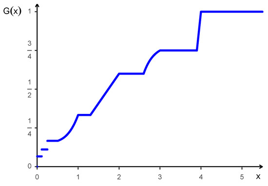
Let the interarrival times $X_i$, $i\in \mathbb{N}$, have a uniform distribution on the interval $[1,1.3]$ with a density function f given by $f\left(x\right)=\frac{10}{3}{\mathbb{1}}_{[1,1.3]}\left(x\right)$, $x\in \mathbb{R}$. Furthermore, let the random inspection time T have the left-continuous distribution function G given in Figure 3. The function G is constant on the interval $[1,1.3]$, i.e., on the support of $X_1$, and therefore, an application of Lemma 1 yields covariance $\mathrm{Cov}(X_1,G\left(X_1\right))=0$. Similarly, G is constant on the support of the occurrence times $S_2$, $S_3$, … from which equality in Equation (5) follows for any choice of φ. In between the supports of $S_n$ and $S_{n+1}$, $n\in \mathbb{N}$, the form of the distribution function G (left-continuous version) is arbitrary.

Figure 3. A distribution function G with non-occurrence of the inspection paradox.

The equality in Example 1 can also be derived by applying Lemma 1. This approach facilitates finding new explicit examples with equality—especially in the case of random inspection times which allow for other possibilities than in the classical inspection paradox with a degenerate time $T\sim {ϵ}_t$.

4. Non-Occurrence of the Inspection Paradox

A general result regarding non-occurrence of the inspection paradox can be derived on the basis of Representation (5) with a random inspection time. This is realised in Theorem 1 and the result is applied to the special cases of equality in (3) and (4); see SubSection 4.2 and Remark 3, respectively. Either result can be used to decide whether a strict inequality holds for specific choices of distribution functions F and G. In particular, the condition for equality is easy to check and can therefore be utilized without calculating, e.g., the expected value of $X_{N\left(T\right)+1}$ explicitly.

4.1. General Results

This subsection is concerned with determining distributions for $X_1$ and T with distribution functions F and G, respectively, such that $E\phi \left(X_{N\left(T\right)+1}\right)=E\phi \left(X_1\right)$ holds, given that $\phi$ is not a constant function. Lemma 2 serves as a key component in the discussion and states that given the support endpoints of the interarrival times, we can explicitly calculate the smallest index n for which the succeeding occurrence times $S_n$ have overlapping supports.

Throughout, $\alpha$ is called an atom of (the distribution of) $X_1$ if $P(X_1=\alpha )>0$.

Lemma 2.

Let the interarrival times have a left support endpoint $\alpha >0$ and right support endpoint $\omega >\alpha$. Then, there exists a natural number $\kappa \in {\mathbb{N}}_0$ at which the supports of two consecutive occurrence times $S_n$ and $S_{n+1}$, $n\ge \kappa +1$, overlap in the sense that $P\left(\right[n\alpha ,n\omega ]\cap [(n+1)\alpha ,(n+1)\omega \left]\right)>0$. In particular, κ is given by

$$\kappa \left\{\begin{array}{cc}{\displaystyle ⌊\frac{\alpha }{\omega -\alpha }⌋,}\hfill & \mathit{if}\omega \ne \frac{k+1}{k}\alpha ,k\in \mathbb{N},\hfill \\ k,\hfill & \mathit{if}\omega =\frac{k+1}{k}\alpha \mathit{for}\mathit{some}k\in \mathbb{N}\mathit{and}\alpha \mathit{and}\mathit{\omega }\mathit{are}\mathit{no}\mathit{atoms}\mathit{of}{X}_1,\hfill \\ k-1,\hfill & \mathit{if}\omega =\frac{k+1}{k}\alpha \mathit{for}\mathit{some}\mathit{k}\in \mathbb{N}\mathit{and}\alpha \mathit{or}\omega \mathit{are}\mathit{atoms}\mathit{of}{X}_1.\hfill \end{array}\right.$$

Proof. 

Assuming that there is no point of overlap for any $n\in \mathbb{N}$, i.e., that

$$n\omega <(n+1)\alpha \mathrm{for}\mathrm{all}n\in \mathbb{N}$$

leads to $\omega \le \underset{n\to \infty }{lim}\frac{n+1}{n}\alpha =\alpha$ which is a contradiction to the assumption that $\alpha <\omega$. Therefore, there exists a natural number for which the supports of successive occurrence times with large enough indices overlap. If $\omega \ne \frac{k+1}{k}\alpha$ for some $k\in \mathbb{N}$, then

$$n\omega -(n+1)\alpha >0⟺n\ge ⌊\frac{\alpha }{\omega -\alpha }⌋+1.$$

If the right support endpoint $\omega$ is of the form $\omega =\frac{k+1}{k}\alpha$ for some $k\in \mathbb{N}$ and $\alpha$ or $\omega$ is an atom of $X_1$, then the first point of overlap is at $(k+1)\alpha =k\omega$, i.e., the supports of $S_k$ and $S_{k+1}$ touch ($\kappa =k-1$). If neither $\alpha$ nor $\omega$ are atoms of $X_1$, then the first overlap happens for the supports of $S_{k+1}$ and $S_{k+2}$ (i.e., $\kappa =k$). □

The trivial case $\alpha =0$ is excluded in Lemma 2 as the support of $X_1$, covered by the interval $[0,\omega ]$ (or $[0,\infty )$), is a subset of the support of $S_n$, covered by $[0,n\omega ]$ (or $[0,\infty )$), for all $n\in \mathbb{N}$. In this case, the supports of all occurrence times overlap.

We will now determine cases with equality of the expected values in (5), i.e., non-occurrence of the inspection paradox, under the general assumption that G is a left-continuous distribution function.

Theorem 1.

Let the interarrival times ${\left(X_i\right)}_{i\in \mathbb{N}}$ have left support endpoint $\alpha >0$, finite right support endpoint $\omega >\alpha$ and let κ be defined as in Lemma 2.

Let $\phi :[0,\infty )\to [0,\infty )$ be a measurable, monotone non-decreasing function such that all expected values and integrals are well-defined and exist finitely. Furthermore, assume that φ is not constant on $\mathcal{S}$$P^{X_1}$-almost surely.

Let T be a non-negative random variable with left-continuous distribution function G that is independent of the interarrival times ${\left(X_i\right)}_{i\in \mathbb{N}}$.

Then, $E\phi \left(X_{N\left(T\right)+1}\right)=E\phi \left(X_1\right)$ is equivalent to

$$\begin{array}{cccc}\hfill \left(i\right)& G\left(x\right)=\sum _{j=0}^{\kappa }{g}_j\left(x\right){\mathbb{1}}_{(j\omega ,(j+1\left)\alpha \right]}\left(x\right)+\sum _{j=1}^{\kappa }{c}_j{\mathbb{1}}_{(j\alpha ,j\omega ]}\left(x\right)+{\mathbb{1}}_{\left(\right(\kappa +1)\alpha ,\infty )}\left(x\right),x\in \mathbb{R},\hfill & \hfill & \\ \hfill & \mathit{if}\alpha \mathit{is}\mathit{no}\mathit{atom}\mathit{of}{X}_1,\hfill & \hfill & \\ \hfill \left(\mathit{ii}\right)& G\left(x\right)=\sum _{j=0}^{\kappa }{g}_j\left(x\right){\mathbb{1}}_{(j\omega ,(j+1\left)\alpha \right]}\left(x\right)+\sum _{j=1}^{\kappa }{c}_j{\mathbb{1}}_{[j\alpha ,j\omega ]}\left(x\right)+{\mathbb{1}}_{\left[\right(\kappa +1)\alpha ,\infty )}\left(x\right),x\in \mathbb{R},\hfill & \hfill & \\ \hfill & \mathit{if}\alpha \mathit{is}\mathit{an}\mathit{atom}\mathit{of}{X}_1,\hfill & \hfill \end{array}$$

(7)

where $0\le c_1\le \dots \le c_{\kappa }\le 1$ are constants and $g_j:(j\omega ,(j+1)\alpha ]\to [0,1]$, $j=0,\dots ,\kappa$, are functions such that G is a left-continuous distribution function.

If $\omega =\infty$, then $E\phi \left(X_{N\left(T\right)+1}\right)=E\phi \left(X_1\right)$ is equivalent to $G\left(x\right)=g_0\left(x\right){\mathbb{1}}_{(0,\alpha ]}\left(x\right)+{\mathbb{1}}_{(\alpha ,\infty )}\left(x\right)$, $x\in \mathbb{R}$, if α is not an atom of $X_1$, and to $G\left(x\right)=g_0\left(x\right){\mathbb{1}}_{(0,\alpha ]}\left(x\right)+{\mathbb{1}}_{[\alpha ,\infty )}\left(x\right)$, $x\in \mathbb{R}$, $g_0\left(\alpha \right)=1$, if α is an atom of $X_1$.

Proof. 

With Equation (5), $E\phi \left(X_{N\left(T\right)+1}\right)=E\phi \left(X_1\right)$ is equivalent to

$$\sum _{n=1}^{\infty }\mathrm{Cov}(\phi \left(X_n\right),G\left(S_n\right))=0⟺\mathrm{Cov}(\phi \left(X_n\right),G\left(S_n\right))=0\mathrm{for}\mathrm{all}n\in \mathbb{N},$$

since $\phi$ and G are both monotone non-decreasing, and thus all covariances are non-negative. For $n=1$, applying Lemma 1 yields

$$\begin{array}{c}\hfill \mathrm{Cov}(\phi \left(X_1\right),G\left(X_1\right))=0⟺G\left(x\right)=c_1\mathrm{for}{P}^{X_1}-\mathrm{almost}\mathrm{all}x\in \mathcal{S}\end{array}$$

for some constant $c_1\in [0,1]$ due to the assumption that $\phi$ is not constant on $\mathcal{S}$$P^{X_1}$-almost surely. First, assume that $P(X_1=\alpha )=0$, i.e., $\alpha$ is not an atom of $X_1$. Since G as a distribution function is monotone non-decreasing and assumed to be left-continuous, we have $G\left(x\right)=c_1$ for all $\alpha <x\le \omega$. With the same arguments, we obtain for a general $n\ge 2$

$$\begin{array}{cc}\hfill \mathrm{Cov}(\phi \left(X_n\right),G\left(S_n\right))=0& ⟺{\int }_0^{\infty }\underset{\ge 0}{\underbrace{\mathrm{Cov}(\phi \left(X_n\right),G(x+X_n))}}d{F}^{*(n-1)}\left(x\right)=0\hfill \\ \hfill & ⟺\mathrm{Cov}(\phi \left(X_n\right),G(x+X_n))=0\mathrm{for}{P}^{S_{n-1}}-\mathrm{almost}\mathrm{all}\hfill \\ \hfill & x\in \mathrm{supp}\left(S_{n-1}\right)\hfill \\ \hfill & ⟺G(x+y)=c_n\mathrm{for}{P}^{X_n}-\mathrm{almost}\mathrm{all}y\in \mathcal{S}\mathrm{and}\hfill \\ \hfill & \mathrm{for}{P}^{S_{n-1}}-\mathrm{almost}\mathrm{all}x\in \mathrm{supp}\left(S_{n-1}\right),\hfill \end{array}$$

for a constant $c_n\in [0,1]$ by using Lemma 1. This implies $G(x+y)=c_n$ for all $n\alpha <x+y\le n\omega$, due to the monotonicity and continuity of the distribution function G. Furthermore, the sequence of constants ${\left(c_n\right)}_{n\in \mathbb{N}}$ needs to satisfy $c_1\le \dots \le c_n$ for all $n\in \mathbb{N}$ (since G is monotone non-decreasing) and $\underset{n\to \infty }{lim}{c}_n=1$ (since $\underset{x\to \infty }{lim}G\left(x\right)=1$).

With Lemma 2, $\kappa +1\in \mathbb{N}$ is the index where the supports overlap, and thus $c_{n+1}=c_{n+2}=\dots =1$ for all $n\ge \kappa$. If $\omega =\infty$, then $\kappa =0$, and thus the distribution function G has to be of the form $G\left(x\right)=g_0\left(x\right){\mathbb{1}}_{(0,\alpha ]}\left(x\right)+{\mathbb{1}}_{(\alpha ,\infty )}\left(x\right)$, $x\in \mathbb{R}$. Otherwise, the distribution function G has to be of the form

$$G\left(x\right)=\left\{\begin{array}{cc}0,\hfill & x\le 0,\hfill \\ g_0\left(x\right),\hfill & 0<x\le \alpha ,\hfill \\ c_1,\hfill & \alpha <x\le \omega ,\hfill \\ g_1\left(x\right),\hfill & \omega <x\le 2\alpha ,\hfill \\ c_2,\hfill & 2\alpha <x\le 2\omega ,\hfill \\ ⋮\hfill & ⋮\hfill \\ c_{\kappa },\hfill & \kappa \alpha <x\le \kappa \omega ,\hfill \\ g_{\kappa }\left(x\right),\hfill & \kappa \omega <x\le (\kappa +1)\alpha ,\hfill \\ 1,\hfill & x>(\kappa +1)\alpha ,\hfill \end{array}\right.$$

where $0=:c_0\le c_1\le \dots \le c_{\kappa }\le c_{\kappa +1}:=1$ and $g_j:(j\omega ,(j+1)\alpha ]\to [0,1]$, $j=0,\dots ,\kappa$, are functions such that $c_j\le g_j\left(x\right)\le c_{j+1}$ for all $j\omega <x\le (j+1)\alpha$, $j=0,\dots ,\kappa$, and such that $g_0,\dots ,g_{\kappa }$ are monotone non-decreasing and left-continuous.

If $P(X_1=\alpha )>0$, then $G\left(x\right)=c_n$ necessarily has to hold for all $n\alpha \le x\le n\omega$, $n\in \mathbb{N}$. Thus, for G as in (7) to be left-continuous at the points $\alpha ,\dots ,(\kappa +1)\alpha$, the additional assumption $g_j\left((j+1)\alpha \right)=c_{j+1}$, $j=0,\dots ,\kappa$, is needed.

For the opposite implication, noticing that G as in (7) is constant on the support of all occurrence times and applying Lemma 1, we see that the covariances $\mathrm{Cov}(\phi \left(X_n\right),G\left(S_n\right))$ are all equal to zero. This leads to equality of the expected values. □

We note that the constant $\kappa$ as introduced in Lemma 2 indicates the kind of support the interarrival times have. For example, $\kappa =0$ can correspond to the case $0<2\alpha <\omega$, where $\omega$ may be infinite. In this case, the distribution of the random inspection time T can be chosen as $T\sim {ϵ}_0$, $T\sim {ϵ}_{\alpha }$ or $T\sim \mathrm{twopoint}\{0,\alpha \}$ among others. On the other hand, $\omega$ must be finite for $\kappa \ge 1$.

Remark 1.

The case $X_1\sim {ϵ}_{\alpha }$ for $\alpha >0$ (which would correspond to $\alpha =\omega$ in Theorem 1) is excluded, because it is already well-known from the literature (cf. Section 2) that $X_{N\left(t\right)+1}\sim X_1$ and that the expected values are always equal, i.e.,

$$E\phi \left(X_{N\left(t\right)+1}\right)=E\phi \left(X_1\right)\mathit{for}\mathit{all}t\ge 0.$$

The equality remains when introducing a random variable T. This can also be derived with the following argument: If $X_1\sim {ϵ}_{\alpha }$, then $S_n\sim {ϵ}_{n\alpha }$ for all $n\in \mathbb{N}$ implies $\mathrm{Cov}(\phi \left(X_n\right),G\left(S_n\right))=0$ for all $n\in \mathbb{N}$ and for any choice of the distribution function G, leading to equality for any φ.

Theorem 1 can be applied to any interarrival distribution. In particular, only the left support endpoint $\alpha$ and the right support endpoint $\omega$ of the interarrival times are of interest. Given a specific interarrival distribution and a distribution function G, Theorem 1 establishes whether or not the inspection paradox occurs.

Example 3.

The case $\omega =2\alpha$ is a particular one (see Lemma 2 with $k=1$). According to Theorem 1 where α is supposed to not be an atom of $X_1$, i.e., $\kappa =1$, the inspection paradox does not occur if G is given by

$$G\left(x\right)=g_0\left(x\right){\mathbb{1}}_{(0,\alpha ]}\left(x\right)+c_1{\mathbb{1}}_{(\alpha ,2\alpha ]}\left(x\right)+{\mathbb{1}}_{(2\alpha ,\infty )}\left(x\right),x\ge 0,$$

with $g_0$ and $c_1$ chosen such that G is left-continuous.

Here, for $\alpha =1$, T may have a two-point distribution on $\mathcal{S}=\{1,2\}$ and $X_1$ may be uniformly distributed on the interval $(1,2)$.

In the case of α being an atom of $X_1$, i.e., $\kappa =0$, G is given by

$$G\left(x\right)=g_0\left(x\right){\mathbb{1}}_{(0,\alpha ]}\left(x\right)+{\mathbb{1}}_{[\alpha ,\infty )}\left(x\right),x\ge 0,$$

and $g_0\left(\alpha \right)=1$ has to be fulfilled.

Furthermore, the following example derived from the results of Theorem 1 shows that, in the degenerate time case with $T\sim {ϵ}_t$, equality in (1) or (2) can also take place for non-degenerate interarrival times. Nevertheless, this situation is irrelevant, since the inspection time coincides with the lower bound of the support of $X_1$.

Example 4.

For absolutely continuous interarrival times with a left endpoint $\alpha :=t>0$ (i.e., α is not an atom of $X_1$) and right endpoint $\omega >2t$, which corresponds to the case $\kappa =0$, we have equality $E\phi \left(X_{N\left(t\right)+1}\right)=E\phi \left(X_1\right)$ for any φ satisfying the assumptions of Theorem 1, since $G\left(x\right)={\mathbb{1}}_{(t,\infty )}\left(x\right)$, $x\ge 0$, is of the form (7) with $g_0\equiv 0$.

Therefore, choosing $\phi \left(x\right)={\mathbb{1}}_{(z,\infty )}\left(x\right)$ and $\phi \left(x\right)=x$ for $x\ge 0$ in Theorem 1, we obtain an example for which

$$\begin{array}{c}\hfill P(X_{N\left(t\right)+1}>z)=P(X_1>z),z\ge 0,\mathit{and}E{X}_{N\left(t\right)+1}=E{X}_1,\mathit{respectively},\end{array}$$

holds even though the interarrival times have a distribution other than the degenerate distribution. Consequently, requiring equality for a single z and t is not sufficient in general to derive a characterization for the distribution of the interarrival times. This case will be considered in detail in Section 5.

The case $\alpha =0$ that was not included in Theorem 1 is studied separately in the following theorem.

Theorem 2.

Let the non-degenerate interarrival times have a left support endpoint $\alpha =0$, where $P(X_1=0)=0$. Let $\phi :[0,\infty )\to [0,\infty )$ be a measurable, monotone non-decreasing function such that all expected values and integrals are well-defined and exist finitely. Furthermore, assume that φ is not constant on $\mathcal{S}:=\mathrm{supp}\left(X_1\right)$$P^{X_1}$-almost surely.

Let T be a non-negative random variable with a left-continuous distribution function G that is independent of the interarrival times ${\left(X_i\right)}_{i\in \mathbb{N}}$.

Then, $E\phi \left(X_{N\left(T\right)+1}\right)=E\phi \left(X_1\right)$ holds if and only if T has a degenerate distribution in 0 for every $\omega >0$.

Proof. 

Analogously to the proof of Theorem 1, $G\left(x\right)=c_n$ must hold for all $0<x\le n\omega$ and for all $n\in \mathbb{N}$, wherefore we obtain $c_1=\dots =c_n=1$ for all $n\in \mathbb{N}$. Thus, G is a distribution function of the degenerate distribution in 0. The opposite direction follows directly from an application of Lemma 1. □

Remark 2.

If $pP(X_1=0)>0$ in Theorem 2 and $G\left(x\right)={\mathbb{1}}_{(0,\infty )}\left(x\right)$ is the left-continuous version of the distribution function of the degenerate distribution in 0, then the first covariance $\mathrm{Cov}(\phi \left(X_1\right),G\left(X_1\right))$ is positive and an inspection paradox occurs. This is the case as G is not constant $P^{X_1}$-almost surely on the support of the interarrival times.

In the above situation with $\phi \left(x\right)=x$ and $P(X_1=1)=1-p$, we find

$$P(N\left(0\right)=k)=p^k,k\in \mathbb{N},\mathit{and}P(N\left(0\right)=0)=1-p,$$

and thus $E{X}_{N\left(0\right)+1}=1-p+p^2>1-p=E{X}_1$.

4.2. Equality of the Survival Functions

Choosing $\phi \left(x\right)={\mathbb{1}}_{(z,\infty )}\left(x\right)$, $x\ge 0$, $z\ge 0$, in Theorem 1 yields distributions with equality in the inspection paradox, in the sense that $P(X_{N\left(T\right)+1}>z)=P(X_1>z)$. In general, a random inspection time T having a distribution function of the particular form (7) is sufficient for equality in the inspection paradox. More precisely, the inspection paradox does not appear in this case and both random variables $X_{N\left(T\right)+1}$ and $X_1$ are identically distributed, as stated in the following corollary.

Corollary 1.

Let the interarrival times have a left support endpoint $\alpha >0$ and right support endpoint $\omega >\alpha$. If T has a distribution function of the form (7), then

$$P(X_{N\left(T\right)+1}>z)=P(X_1>z)\mathit{for}\mathit{all}z\ge 0,$$

i.e., $X_{N\left(T\right)+1}{=}_{\mathrm{st}}{X}_1$.

Proof. 

Since the G given in (7) is constant on the supports of $X_n$ and of $S_n$ for all $n\in \mathbb{N}$, applying Lemma 1 yields $\mathrm{Cov}({\mathbb{1}}_{(z,\infty )}\left(X_n\right),G\left(S_n\right))=0$ for all $n\in \mathbb{N}$ and for all $z\ge 0$ as in the proof of Theorem 1. Therefore, with

$$P(X_{N\left(T\right)+1}>z)=P(X_1>z)+\underset{=0}{\underbrace{\sum _{n=1}^{\infty }\mathrm{Cov}({\mathbb{1}}_{(z,\infty )}\left(X_n\right),G\left(S_n\right))}}\mathrm{for}\mathrm{all}z\ge 0,$$

$X_{N\left(T\right)+1}$ and $X_1$ are identically distributed. □

In the characterization of Theorem 1, the function $\phi$ is assumed to be non-constant on $\mathcal{S}$$P^{X_1}$-almost surely. Therefore, for the function ${\mathbb{1}}_{(z,\infty )}(·)$ to take both values 0 and 1 on the support of $X_1$ with positive probability, we require $z\in \mathrm{supp}\left(X_1\right)$.

Corollary 2.

Let the interarrival times have a left support endpoint $\alpha >0$, right support endpoint $\omega >\alpha$ and let $\mathcal{S}:=\mathrm{supp}\left(X_1\right)$. Let T be a non-negative random variable with left-continuous distribution function G that is independent of the interarrival times ${\left(X_i\right)}_{i\in \mathbb{N}}$. If there is a $z\in \mathcal{S}$ such that ${\mathbb{1}}_{(z,\infty )}(·)$ takes both values 0 and 1 on $\mathcal{S}$ with positive probability and

$$P(X_{N\left(T\right)+1}>z)=P(X_1>z),$$

then G is of the form (7).

Proof. 

This follows from Theorem 1 for the choice $\phi \left(x\right)={\mathbb{1}}_{(z,\infty )}\left(x\right)$, $x\ge 0$. □

Corollary 2 shows that equality for an appropriate value of z is enough to determine the general form of the distribution function G (on finite intervals). Thus, if we have equality of the survival functions of $X_{N\left(T\right)+1}$ and $X_1$ for this $z\in \mathcal{S}$, then T is of the form (7) and Corollary 1 yields $X_{N\left(T\right)+1}{=}_{\mathrm{st}}{X}_1$.

Remark 3.

The inspection paradox is also discussed in terms of expected values, as we have seen in Section 2 and Section 3. With the choice $\phi \left(x\right)=x$, $x\ge 0$, it follows under the assumptions of Theorem 1 that equality of the expected values $E{X}_{N\left(T\right)+1}=E{X}_1$ holds if and only if G is of the form (7).

Similarly, equality of the moments, i.e., $E\left(X_{N\left(T\right)+1}^m\right)=E\left(X_1^m\right)$, also determines the distribution of T. This can be obtained from Theorem 1 via the choice $\phi \left(x\right)=x^m$, $x\ge 0$, $m>0$.

5. Equality in the Degenerate Time Case

As discussed in Section 2 and in Remark 1, no paradoxical effect appears for the inspection interval length given degenerate interarrival times, regardless of whether the inspection time is random or deterministic. On the other hand, degenerate interarrival times are not the only example with this property (cf. Example 4). In this section, we further study equality in the inspection paradox by means of a fixed sequence of inspection times.

The following Theorem 3 states that having such a sequence of fixed times for which equality holds is sufficient for the interarrival times to have a degenerate distribution.

Theorem 3.

Let the interarrival times ${\left(X_i\right)}_{i\in \mathbb{N}}$ have a distribution function F with $F\left(0\right)<1$. Let ${\left(t_i\right)}_{i\in \mathbb{N}}\subseteq (0,\infty )$ be a sequence of monotone increasing times ($t_i<t_{i+1}$, $i\in \mathbb{N}$) with $\underset{i\to \infty }{lim}{t}_i=\infty$, such that

$$E{X}_{N\left(t_i\right)+1}=E{X}_1\mathit{for}\mathit{all}i\in \mathbb{N}.$$

Then, $X_1=\alpha$ almost surely for some $\alpha >0$, i.e., $F\left(x\right)={\mathbb{1}}_{[\alpha ,\infty )}\left(x\right)$, $x\ge 0$.

Proof. 

We assume that the interarrival times have a left support endpoint $\alpha \ge 0$ and right support endpoint $\omega >\alpha$ and define $\mathcal{S}:=[\alpha ,\omega ]$ if $\omega <\infty$ and $\mathcal{S}=[\alpha ,\infty )$ if $\omega =\infty$. Thus, it is assumed that the support contains at least two values and this is shown to lead to a contradiction in the following. Due to Representation (6) with $T\sim {ϵ}_{t_i}$, equality holds if and only if

$$\begin{array}{c}\hfill \mathrm{Cov}(X_n,{\mathbb{1}}_{(t_i,\infty )}\left(S_n\right))=0\mathrm{for}\mathrm{all}n\in \mathbb{N}\mathrm{and}\mathrm{for}\mathrm{all}i\in \mathbb{N}.\end{array}$$

In the case $n=1$, an application of Lemma 1 yields

$$\begin{array}{cc}\hfill & \mathrm{Cov}(X_1,{\mathbb{1}}_{(t_i,\infty )}\left(X_1\right))=0\mathrm{for}\mathrm{all}n\in \mathbb{N}\mathrm{and}\mathrm{for}\mathrm{all}i\in \mathbb{N}\hfill \\ \hfill ⟺& {\mathbb{1}}_{(t_i,\infty )}\left(x\right)=\mathit{const}\mathrm{for}{P}^{X_1}-\mathrm{almost}\mathrm{all}x\in \mathcal{S}\mathrm{and}\mathrm{for}\mathrm{all}i\in \mathbb{N}.\hfill \end{array}$$

(8)

From (8), we obtain that $\mathcal{S}$ necessarily has to lie in a bounded interval, i.e., $\omega <\infty$. Let ${\mathcal{S}}_n[n\alpha ,n\omega ]$, $n\in \mathbb{N}$. As in the proof of Theorem 1, the case $n\ge 2$ leads to

$$\begin{array}{cc}\hfill {\mathbb{1}}_{(t_i,\infty )}(x+y)=\mathit{const}& \mathrm{for}{P}^{X_n}-\mathrm{almost}\mathrm{all}x\in \mathcal{S},\hfill \\ \hfill & \mathrm{for}{P}^{S_{n-1}}-\mathrm{almost}\mathrm{all}y\in {\mathcal{S}}_{n-1}\mathrm{and}\mathrm{for}\mathrm{all}i\in \mathbb{N}.\hfill \end{array}$$

Due to Lemma 2, there exists a $\kappa \in {\mathbb{N}}_0$ such that $P\left(\right[n\alpha ,n\omega ]\cap [(n+1)\alpha ,(n+1)\omega \left]\right)>0$ for all $n\ge \kappa +1$. This implies

$$\bigcup _{n\ge \kappa +1}[n\alpha ,n\omega ]=[(\kappa +1)\alpha ,\infty ),$$

i.e., the supports of $S_{\kappa +1}$, $S_{\kappa +2}$, … cover all real numbers greater than or equal to $(\kappa +1)\alpha$. Since the unbounded sequence ${\left(t_i\right)}_{i\in \mathbb{N}}$ consists of monotone increasing real numbers, there exists a smallest $k\in \mathbb{N}$ with $t_k>(\kappa +1)\alpha$ and an $n\in \mathbb{N}$ with $n\ge \kappa +2$ such that $t_k\in [n\alpha ,n\omega ]$.

If $n\alpha <t_k<n\omega$, then the indicator function

$${\mathbb{1}}_{(t_k,\infty )}(x+y)=\left\{\begin{array}{cc}0,\hfill & x\in \mathcal{S}\mathrm{and}y\in (n\alpha -x,t_k-x],\hfill \\ 1,\hfill & x\in \mathcal{S}\mathrm{and}y\in (t_k-x,n\omega -x],\hfill \end{array}\right.,\mathrm{i}.\mathrm{e}.,x+y\in {\mathcal{S}}_n,$$

has a jump and is not constant for $P^{X_n}$-almost all $x\in \mathcal{S}$ and $P^{S_{n-1}}$-almost all $y\in {\mathcal{S}}_{n-1}$. Concerning the occurrence time $S_n$, we obtain $\mathrm{Cov}(X_n,{\mathbb{1}}_{(t_k,\infty )}\left(S_n\right))>0$, which is in contradiction to the assumed equality.

If $t_k=n\alpha$, then $t_k$ lies in the preceding interval with $(n-1)\alpha <t_k<(n-1)\omega$, since this interval overlaps with the interval $[n\alpha ,n\omega ]$ due to $n-1\ge \kappa +1$. Again, the indicator function ${\mathbb{1}}_{(t_k,\infty )}(·)$ is not constant for $P^{X_{n-1}}$-almost all $x\in \mathcal{S}$ and $P^{S_{n-2}}$-almost all $y\in {\mathcal{S}}_{n-2}$. In consequence, $\mathrm{Cov}(X_{n-1},{\mathbb{1}}_{(t_k,\infty )}\left(S_{n-1}\right))>0$ is a contradiction to the equality.

If $t_k=n\omega$, then $t_k$ lies in the subsequent interval $(n+1)\alpha <t_k<(n+1)\omega$, which implies $\mathrm{Cov}(X_{n+1},{\mathbb{1}}_{(t_k,\infty )}\left(S_{n+1}\right))>0$, leading to a contradiction.

In conclusion, $\left|\mathcal{S}\right|=1$ must hold $P^{X_1}$-almost surely and there exists an $\alpha >0$ with $X_1=\alpha$ almost surely and $F\left(x\right)={\mathbb{1}}_{[\alpha ,\infty )}\left(x\right)$, $x\ge 0$. The constant $\alpha$ has to be positive due to $F\left(0\right)<1$. □

Note that having only a finite number of times $t_i$ with equality in Theorem 3 does not suffice to derive that the interarrival times have a degenerate distribution. If there was a largest $t_N<\infty$, then $X_1$ could have a support lying to the right of $t_N$ and consisting of more than one number and we would still have equality.

The same arguments as in Theorem 3 lead to an analogous result in case of the classical inspection paradox inequality for a sequence of time points. In a similar way to the main result in Section 4, Theorem 3 and the following Corollary 3 can be combined by using a function $\phi$ that is assumed to be not constant almost surely on the support of the interarrival times.

Corollary 3.

Let the interarrival times ${\left(X_i\right)}_{i\in \mathbb{N}}$ have the distribution function F with $F\left(0\right)<1$. Let ${\left(t_i\right)}_{i\in \mathbb{N}}\subseteq (0,\infty )$ be a sequence of monotone increasing times ($t_i<t_{i+1}$, $i\in \mathbb{N}$) with $\underset{i\to \infty }{lim}{t}_i=\infty$. Let $z\in \mathcal{S}:=\mathrm{supp}\left(X_1\right)$ such that ${\mathbb{1}}_{(z,\infty )}(·)$ takes values 0 and 1 on $\mathcal{S}$ with positive probability and

$$P(X_{N\left(t_i\right)+1}>z)=P(X_1>z)\mathit{for}\mathit{all}i\in \mathbb{N}.$$

Then, $X_1=\alpha$ almost surely for some $\alpha >0$, i.e., $F\left(x\right)={\mathbb{1}}_{[\alpha ,\infty )}\left(x\right)$, $x\ge 0$.

We note that in both Theorem 3 and Corollary 3, we did not assume that any particular point $t_i$ lies in the support of an occurrence time, as this assumption alone does not suffice (in Example 4, the time t lies in the support of $X_1$). In order to infer that the interarrival times have a degenerate distribution based on only one time point t, it is necessary to assume that t lies in the support of an occurrence time whose support overlaps with both the support of the preceding and the succeeding occurrence time. This is formally stated in Corollary 4.

Corollary 4.

Let the interarrival times ${\left(X_i\right)}_{i\in \mathbb{N}}$ have a distribution function F with $F\left(0\right)<1$. Assume that there exists a $k\in \mathbb{N}$ with $k\ge \kappa +2$ and a $t>0$ such that $t\in \mathrm{supp}\left(S_k\right)$. Then,

$$E{X}_{N\left(t\right)+1}=E{X}_1$$

implies $X_1=t/k$ almost surely, i.e., $F\left(x\right)={\mathbb{1}}_{[t/k,\infty )}\left(x\right)$, $x\ge 0$.

Proof. 

Due to the equality of the expected values and to Representation (6), the covariances $\mathrm{Cov}(X_n,{\mathbb{1}}_{(t,\infty )}\left(S_n\right))$ must be equal to zero for all $n\in \mathbb{N}$. Assume that the support of $S_k$ contains at least two different points, then $P(\mathrm{supp}\left(S_{k-1}\right)\cap \mathrm{supp}\left(S_k\right))>0$ and $P(\mathrm{supp}\left(S_k\right)\cap \mathrm{supp}\left(S_{k+1}\right))>0$ holds due to Lemma 2. As in the proof of Theorem 3, we can infer that t lies in the inner of either the support of $S_k$, of $S_{k-1}$ or of $S_{k+1}$, respectively, which leads to a contradiction. Thus, $\mathrm{supp}\left(S_k\right)=t$ implies $P(S_k\le x)={\mathbb{1}}_{[t,\infty )}\left(x\right)$; i.e., $S_k$ has a degenerate distribution in t. Since $S_k$ is the sum of k iid interarrival times, we then have $X_1=t/k$ almost surely. □

6. Conclusions

By considering a random inspection time in a renewal counting process, interesting effects come into play and new insights are gained regarding the distribution of the random time. With respect to the well-known inspection paradox, non-trivial choices of this distribution and the distribution of the interarrival times lead to non-occurrence of the paradox in contrast to the situations for a deterministic time. In the general case, a complete characterization of the (non-)occurrence of the inspection paradox with respect to G is given.

References

- Feller, W. An Introduction to Probability Theory and Its Applications, 2nd ed.; John Wiley & Sons Inc.: New York, NY, USA, 1971; Volume II. [Google Scholar]
- Masuda, N.; Porter, M.A. The waiting-time paradox. Front. Young Minds Math. 2021, 8, 582433. [Google Scholar] [CrossRef]
- Ross, S.M. Introduction to Probability Models, 10th ed.; Academic Press: London, UK, 2010. [Google Scholar]
- Stein, W.E.; Dattero, R. Sampling bias and the inspection paradox. Math. Mag. 1985, 58, 96–99. [Google Scholar] [CrossRef]
- Pal, A.; Kostinski, S.; Reuveni, S. The inspection paradox in stochastic resetting. J. Phys. A Math. Theor. 2022, 55, 021001. [Google Scholar] [CrossRef]
- Jenkins, E.V.; Dharmaprani, D.; Schopp, M.; Quah, J.X.; Tiver, K.; Mitchell, L.; Xiong, F.; Aguilar, M.; Pope, K.; Akar, F.G.; et al. The inspection paradox: An important consideration in the evaluation of rotor lifetimes in cardiac fibrillation. Front. Physiol. 2022, 13, 920788. [Google Scholar] [CrossRef] [PubMed]
- Gakis, K.G.; Sivazlian, B.D. A generalization of the inspection paradox in an ordinary renewal process. Stoch. Anal. Appl. 1993, 11, 43–48. [Google Scholar] [CrossRef]
- Angus, J.E. The inspection paradox inequality. SIAM Rev. Soc. Ind. Appl. Math. 1997, 39, 95–97. [Google Scholar]
- Ross, S.M. The inspection paradox. Probab. Eng. Inf. Sci. 2003, 17, 47–51. [Google Scholar] [CrossRef]
- Kamps, U. Inspection paradox. In Encyclopedia of Statistical Sciences, 3(Update); Kotz, S., Read, C.B., Banks, D.L., Eds.; John Wiley & Sons Inc.: New York, NY, USA, 1999; pp. 364–366. [Google Scholar]
- Herff, W.; Jochems, B.; Kamps, U. The inspection paradox with random time. Stat. Pap. 1997, 38, 103–110. [Google Scholar] [CrossRef]
- Rauwolf, D.; Kamps, U. Quantifying the inspection paradox with random time. Am. Stat. 2023, 77, 274–282. [Google Scholar] [CrossRef]
- Liu, P.; Peña, E.A. Sojourning with the homogeneous Poisson process. Am. Stat. 2016, 70, 413–423. [Google Scholar] [CrossRef] [PubMed]
- Cox, D.R. Renewal Theory; Methuen & Co.: London, UK, 1962. [Google Scholar]
- Pinsky, M.A.; Karlin, S. An Introduction to Stochastic Modeling, 4th ed.; Academic Press: Burlington, VT, USA, 2011. [Google Scholar]
- Mitov, K.V.; Omey, E. Renewal Processes; Springer: Cham, Switzerland, 2014. [Google Scholar]
- Kulkarni, V.G. Modeling and Analysis of Stochastic Systems, 3rd ed.; CRC Press: Boca Raton, FL, USA, 2017. [Google Scholar]
- Behboodian, J. Covariance inequality and its applications. Int. J. Math. Educ. Sci. Technol. 1994, 25, 643–647. [Google Scholar] [CrossRef]
- Rauwolf, D. Renewal Processes with Random Time. Ph.D. Thesis, RWTH Aachen University, Aachen, Germany, 2023. [Google Scholar]
Disclaimer/Publisher’s Note: The statements, opinions and data contained in all publications are solely those of the individual author(s) and contributor(s) and not of MDPI and/or the editor(s). MDPI and/or the editor(s) disclaim responsibility for any injury to people or property resulting from any ideas, methods, instructions or products referred to in the content. |
© 2024 by the authors. Licensee MDPI, Basel, Switzerland. This article is an open access article distributed under the terms and conditions of the Creative Commons Attribution (CC BY) license (https://creativecommons.org/licenses/by/4.0/).