Article

Contrastive Learning Framework for Bitcoin Crash Prediction

1
Department of Applied Mathematics and Statistics, Stony Brook University, Stony Brook, NY 11794, USA
2
Department of Statistics, Actuarial and Data Sciences, Central Michigan University, Mt Pleasant, MI 48859, USA
*
Author to whom correspondence should be addressed.
Stats 2024, 7(2), 402-433; https://doi.org/10.3390/stats7020025
Submission received: 14 January 2024 / Revised: 15 April 2024 / Accepted: 30 April 2024 / Published: 8 May 2024

Abstract

:
Due to spectacular gains during periods of rapid price increase and unpredictably large drops, Bitcoin has become a popular emergent asset class over the past few years. In this paper, we are interested in predicting the crashes of Bitcoin market. To tackle this task, we propose a framework for deep learning time series classification based on contrastive learning. The proposed framework is evaluated against six machine learning (ML) and deep learning (DL) baseline models, and outperforms them by 15.8% in balanced accuracy. Thus, we conclude that the contrastive learning strategy significantly enhance the model’s ability of extracting informative representations, and our proposed framework performs well in predicting Bitcoin crashes.

1. Introduction

Digital coins known as cryptocurrencies have gained popularity over the past ten years due to their enormous return potential during periods of rapid price increase and unanticipated sharp falls. Cryptocurrencies are decentralized using a distributed ledger technology known as blockchain that serves as a public record of financial transactions, in contrast to centralized digital money and central banking systems. The 2008 global financial crisis and the 2010–2013 European sovereign debt crisis were caused by failures of governments and central banks, which led to a surge interest in cryptocurrencies from investors. The most well-known cryptocurrency is Bitcoin, and many private investors’ “fear of losing out” may have contributed to its price climb to about USD 20,000 per coin in December 2017. This raises the question of whether the price behavior of Bitcoin has characteristics of financial bubbles. Hence, there is a rapidly expanding body of research on Bitcoin bubble [1,2,3,4,5], but the topic of bubble behavior is still far from being fully understood.
In the last few years, Deep Learning (DL) has strongly emerged as the best performing predictor class within the Machine Learning (ML) field across various implementation areas. Financial time series forecasting is no exception, and as such, an increasing number of prediction models based on various DL techniques have been introduced in the appropriate conferences and journals in recent years. Sezer et al. [6] systematically reviewed the literature on financial forecasting with deep learning during the period 2005–2019 and concluded that models based on recurrent neural networks (RNNs), such as Long Short-Term Memory (LSTM) and gated recurrent unit (GRU) networks, are the most commonly accepted models because they dominate in price and trend predictions and are easily adapted to a variety of forecasting problems. However, DL models always require large scale labeled dataset for achieving such remarkable performance. It is thus very challenging to apply them to time series data, because generally time series data do not have human recognizable patterns, which make it much harder to label time series data than images, and little time series data have been labeled for practical applications.
To overcome the challenge of limited labeled data, self-supervised learning has recently gained more attention recently to extract effective representations for downstream tasks. Compared with models trained on full labeled data (i.e., supervised models), self-supervised pre-trained models can achieve comparable performance with limited labeled data [7]. Various self-supervised approaches rely on different pretext tasks [8] to train the models and learn representations from unlabeled data. A common pretext task for time series analysis is to train an Autoencoder for reconstruction, and use the final hidden representation as an input for the downstream task of classification or regression, as shown in [9]. As a self-supervised training technique, Contrastive Learning (CL) has recently shown its powerful ability for representation learning because of its ability to learn invariant representation from augmented data [7,10,11]. However, most of the works and applications on Contrastive Learning are in the domain of computer vision, and few are applied to time series data, especially financial data.
In this work, we propose a framework for time series classification framework based on contrastive learning via SimCLR [7]. In order to extract better representations for time series data, we make some modifications—our framework employs simple yet efficient data augmentations that are suitable for time series data, we substitute the encoder of it with a temporal convolutional network (TCN). For the downstream crashes detection task, we employ Epsilon Drawdown Method [12,13] to label the data, and make prediction by using the extracted representations as input and a multilayer perceptron (MLP) as classifier. We test the proposed framework on Bitcoin daily price data, and compare it performance with various ML/DL baseline models. The main contributions of this work are as follows:
  • We propose a deep learning framework based on contrastive learning for extracting latent representations for time series data and tackle downstream time series classification task.
  • We apply the proposed framework to predict crashes of Bitcoin. To the best of our knowledge, we are the first to employ contrastive learning in analyzing cryptocurrencies.
  • We investigate the performance of multiple time series augmentation methods in contrastive learning based model, and the effect of some augmentation parameters.
  • We compare our proposed framework against six state-of-the-art classification models, which include both ML and DL models.
  • We explore the efficacy of ensemble techniques in an effort to improve the overall classification performance.
  • We compare and combine the CL framework with the Log Periodic Power Law Singularity (LPPLS) model, which is also unprecedented, to the best of our knowledge.
The paper is structured as follows. Section 2 reviews several research areas closely related to this paper, providing background information and highlighting Contrastive Learning-based models and their extensions on time series data. Section 3 presents the architecture of our framework and detailed methodologies and procedures employed. Section 4 provides the data in experiments, model implementation, and performance evaluation. Section 5 concludes the paper by summarizing the key findings and contributions of our study.

2. Related Work and Background

In this section, we discuss several research areas that are closely related to our paper, showing not only the background of the fields but also the recent works that make great achievements. These includes the commonly used test for detecting financial bubble, contrastive learning based DL models and their extension on time series data.

2.1. Financial Crashes

Crashes in financial markets are of extreme importance as they may have great impact on the lives and livelihoods of most people all over the world, directly or indirectly. There have been seven distinct crashes in the U.S. financial markets over the past 30 years, including the 1987 stock market crash, the collapse of long-term capital management following the Russian debt crisis and the subsequent market crash of 1998, the bursting of the dotcom bubble during the period of 1999–2001, the financial meltdown following the subprime mortgage crisis during the period from 2007 to 2009, and 2020 stock market crash. In addition, in the past 30 years there are approximately 100 financial crises worldwide [14]. Each crash of bubbles resulted in permanent impairment of wealth, at least for some investors [15]. Because of their great impact, researchers and economists have studied on financial bubbles for many decades, investigating the underlying mechanisms and looking for better ways to predict them.
In the broadest sense, financial bubbles are generally defined as the abnormal accelerating ascent of an asset price above the fundamental value of the asset [16]. When a bubble goes burst, i.e., crash occurs, investors with very little experience of managing risks usually hold the asset at the late phase and thus are damaged by the bubbles excessively [17]. This intuitive description is, however, quite hard to conceptualize and full of traps, as it requires the implicit definition of both ‘abnormal price growth’ and ‘crash’. To measure abnormal price increases, a reference frame or process against which deviations can be gauged, must be defined. However, when employing such a reference process, a bubble may be incorrectly diagnosed due to an inaccurate underlying benchmark model, an issue that makes the diagnostic of a bubble a joint-hypothesis problem. Similarly, a crash is also not easy to define. It can be vaguely described as a mixture of a large loss over some relatively short duration that seems abnormal compared to regular asset price movements.

2.2. Contrastive Learning

The basic concept for contrastive learning was proposed in [18,19], which looked at the comparison of distinct samples without labels. There have been a number of studies since then using a similar principle, which have been surveyed in [20]. In recent years, contrastive learning has risen to prominence as a technique for learning representations from augmented data. Specifically, it uses a set of training instances made up of positive sample pairs (samples that are similar in some way) and negative sample pairs (samples that are different). Within the embedding space, a representation is learned to bring positive sample pairs closer together while also separating negative sample pairs. For instance, MoCo [10] utilized a momentum encoder to learn representations of negative pairs obtained from a memory bank. SimCLR [7] replaced the momentum encoder by using a larger batch of negative pairs. Also, BYOL [11] learned representations by bootstrapping representations even without using negative samples. Last, SimSiam [21] supported the idea of neglecting the negative samples, and relied only on a Siamese network and stop-gradient operation to achieve the state-of-the-art performance. While all of these methods have enhanced representation learning for visual data, they may not function as well on time series data with unique traits such as temporal dependency.

2.3. Contrastive Learning for Time Series

Representation learning for time series is becoming increasingly popular, and few works have recently leveraged contrastive learning for time series data. For example, model CPC [22] learned representations by predicting the future in the latent space and showed great advances in various speech recognition tasks. Also, Ref. [23] designed electroencephalogram (EEG) related augmentations and extended SimCLR model to EEG data. In addition, other works [24,25,26,27,28] applied contrastive learning to improve performance of deep learning models on time series forecasting, classification, or change point detection tasks. They are summarized in Table 1.
From Table 1, we can see that very few studies have applied contrastive learning to financial time series data. One of the first few is [29], which exploited the different efficacy of heterogeneous multigranularity information to construct non-end-to- end multigranularity models for stock price prediction, which can adaptively fuse multigranularity features at each time step and maximize the mutual information between local segments and their global contexts (Context-Instance). Wang et al. [30] applied copula-based CPC architecture to learn a better stock representation with less uncertainty by considering hierarchical couplings from the macro-level to the sector-and micro-level, and used the proposed model for stock movement prediction. Feng et al. [31] utilized contrastive learning to exploit the correlation between intra-day data and enhance stock representation in order to improve the accuracy of stock movement prediction.
However, to the best of our knowledge, there has been no study working on taking advantage of CL to predict bubbles and crashes in assets’ price. Forecasting financial bubbles and crashes has always been a tough but attractive task for researchers in machine learning and data mining. We believe it is worth investigating the CL on various challenging tasks, including bubbles prediction, because it will definitely give researchers a deeper understanding and a wider view on this emerging technique, thus providing chances to improve it and make a better use of it.

3. Methods

In this section, we define the problem we aim to address using the language of machine learning domain, outline the methodology for generating the target labels in the problem, and provide a detailed overview of the proposed framework.

3.1. Problem Definition

For forecasting crashes, we aim to predict if there will be a large crash in the next few days. So, in machine learning field, it can be categorized as a binary classification problems. Formally, the prediction model learns a function y ^ t = F θ ( X t ) , which maps a sequence of the historical stock prices to the label space. Specifically, for current time t, X t T + 1 = [ x t T + 1 , , x t ] R T represents a sequence of stock prices in the lag of past T time-steps. The target label y t has two classes—there is a crash in the next M days or there is not a crash in the next M days. To generate the target label, we apply Epsilon Drawdown Method for identifying crashes in the entire time series.

3.2. The Epsilon Drawdown Method

The Epsilon Drawdown Method is a peak detection algorithm developed by Johansen and Sornette [12,13] and further used in [34,35]. The main goal of Epsilon-drawdown method is to systematically segment a price trajectory into a series of alternating and consecutive price drawup and drawdown phases that are subsequently translated into bubbles and crashes. A drawdown (drawup) is defined as a succession of negative (positive) returns ( ( p t p t 1 ) / ( p t 1 ) ) that may only be interrupted by a positive (negative) return which is larger than the pre-specified tolerance level ϵ . Consequently, the start time of a drawdown is called peak time—when a succession of positive returns followed by a negative return whose amplitude exceeds ϵ . Parameter ϵ controls the degree to which counter-movements in a drawup or drawdown phase are tolerated.
Let parameter ϵ be a function of time t
ε ( t ) = ε 0 σ t ( ω )
where σ t ( ω ) denotes the standard deviation of returns over the past ω days from time t and ε 0 is a constant multiplier. Thus, the counter-movement tolerance dynamically changes over time, instead of being fixed. Once ε 0 and ω is given, a set of the start times of drawdowns (peak times) among the time series data can be obtained.
To collect a robust set of peak times, it is better to run the algorithm with numerous pairs of ( ε 0 , ω ) , and then select the time points that are highly frequently determined as peak time by different pair of parameters. The process can be expressed as that given a set of parameter pairs { ( ε 0 , ω ) i | i = 1 , , N ε } , for each pair ( ε 0 , ω ) i , a set of peak times among the time series (with length of T) can be obtained by the algorithm and denoted it as
I i = { I i , 1 , I i , 2 , , I i , T } , i = 1 , , N ε .
where I i , t is an indicator function
I i , t = 1 , if time t is a peak time determined by ( ε 0 , ω ) i 0 , otherwise .
The frequency of time t being selected as a peak time over all pairs of parameters can be expressed as
n t = i = 1 N ε I i , t
The fraction of occurrence of time t with respect to the total number of trials is
P = { p t = n t N ε | t = 1 , , T } .
This fraction is finally used to filter peaks.

3.3. Model Architecture

We adopt a similar approach to the SimCLR model [7] to extract compact latent representations that maximizes the similarity between positive pairs, however there are variations as we deal with time series data instead of images:
  • for sampling, we apply the augmentations that are not only commonly used for images but also reasonable for time series sequences, maintaining the overall trend of the sequence so as not to change the original input too much;
  • instead of a ResNet-50 [36] architecture, we use a temporal convolutional network (TCN) [37], which is more suitable for time series data;
  • we remain the projection head for the downstream task
The architecture of our approach is depicted in Figure 1. It starts from an input time series window of length T, denoted as X i = [ x i , , x i + T 1 ] R T , from which a positive pair is composed of two equal-length sequences ( I h and I f as shown in Figure 1) that are transformed by augmentation methods from the same original window. The two augmentation methods we take into consideration are transformation functions commonly used for time series [38], including jittering, scaling, magnitude-warping, time-warping, crop-and-resize and Gaussian smoothing. Details of these methods are shown in Section 3.4. Thus, the two augmented sequences of input window X i can be denoted as
h i = Aug h ( [ x i , , x i + T 1 ] ) , f i = Aug f ( [ x i , , x i + T 1 ] )
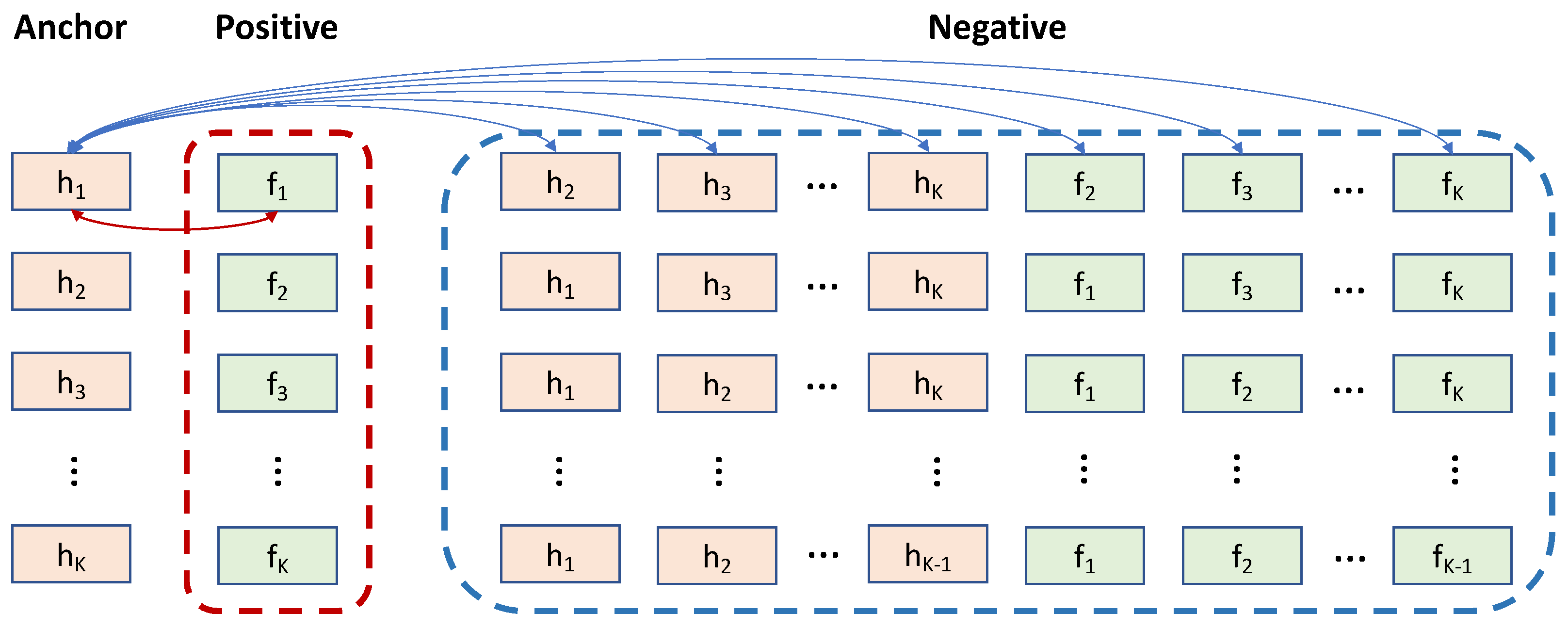
where Aug h and Aug f denote two augmentation methods, therefore h i and f i form a positive pair of samples. In training process, each batch of samples contains K randomly selected positive pairs of windows { ( h i , f i ) | i = 1 , 2 , , K } . To construct negative pairs for the batch, for each anchor sample h i in the batch, we set the remaining 2 K 2 windows as its negative samples, so all the negative pairs can be written as { ( h i , h j ) , ( h i , f j ) | i , j [ 1 , K ] , i j } . The intuition of this sampling procedure is that time series are typically non-stationary, hence samples that are augmented from temporally separated windows are likely to have lower statistical dependencies than those from the same window. Figure 2 visualizes the construction of a batch in our model. A red two-way arrow represents a positive pair of samples, and a blue two-way arrow represents a negative pair of samples.
Given it has been shown in some works [39,40,41,42] that TCN can typically outperform Recurrent Neural Network (RNN)-based Long Short-Term Memory (LSTM) with temporal data on a vast range of tasks and is generally easier and faster in training, we employ TCN as the encoder to compress time windows into embedding representations.
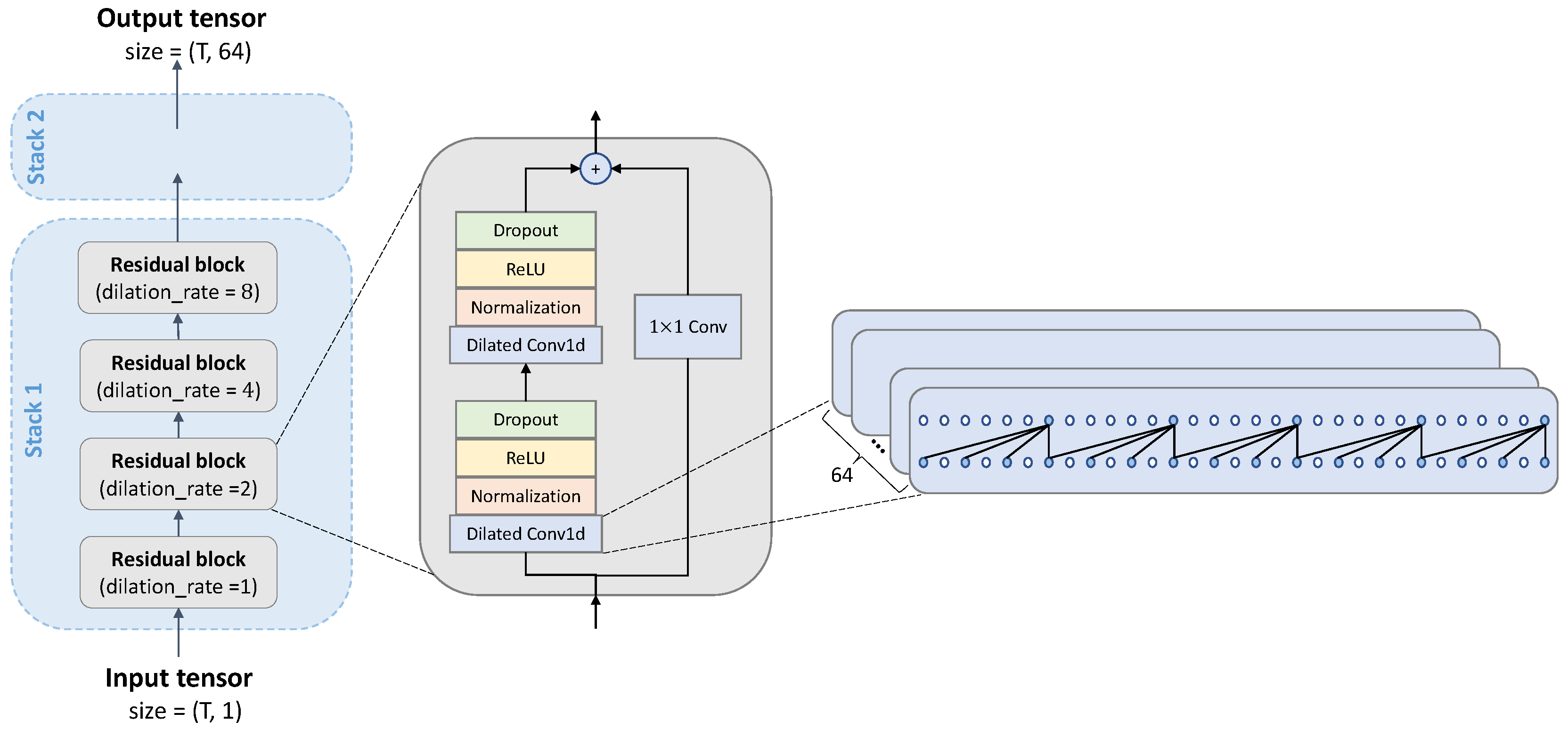
Figure 3 illustrates the encoder architecture we use. It consists of two stacks of TCN (we acknowledge the main illustration and TCN implementation: https://github.com/philipperemy/keras-tcn, accessed on 13 January 2024), each containing 4 residual blocks with respective dilation rates of 1, 2, 4 and 8. Each residual block consists of two dilated causal convolutions with 64 kernel filters of size 4. Batch normalization and Rectified Linear Unit (ReLU) activation function are performed for every convolution layer. According to the architecture, the shape of input data is (N, T, c), where N is the number of windows, T is the length of window, and c denotes the number of channels. Through the entire encoder, the intermediate data has shape (N, T, 64)—the number of channel is increased from 1 to 64, because each dilated convolution layer has 64 filters inside, and each filter generates a single output tensor. In order to match the output shape of encoder to the input of the following projection head, a flatten layer is added between these two parts.
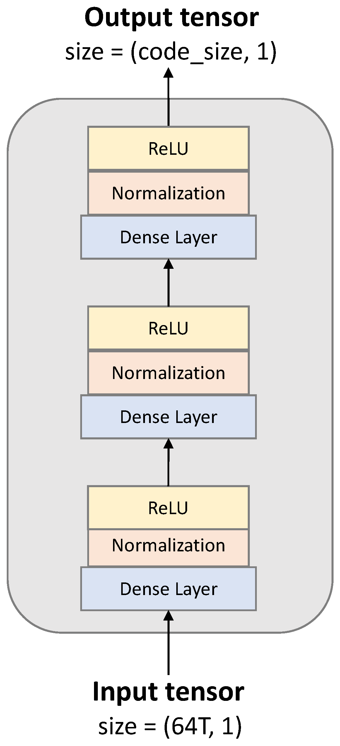
The projection head is used to reduce the encoder’s output dimension to the pre-specified size of desired representation ( c o d e _ s i z e ). To achieve this goal, the projection head is set up as a simple three-layer of multi-layer perceptron (MLP) with ReLU activation function, and output shapes of T, T / 2 and c o d e _ s i z e , respectively. The architecture of projection head is shown in Figure 4.
After passing the augmented tensor through the encoder and the projection head, each positive pair ( h i , f i ) can be converted to its final representation ( h i ˜ , f i ˜ ) , and their similarity is calculated by cosine similarity and written as
sim ( h i ˜ , f i ˜ ) = h i ˜ · f i ˜ | | h i ˜ | | | | f i ˜ | | .
To maximize the similarity of positive pairs and simultaneously minimize the similarity of negative pairs, a Normalized Temperature-scaled Cross Entropy Loss (NT-Xent) [43] is used in the contrastive learning process. The final loss function can be computed as:
L = 1 2 K i = 1 K log exp ( sim ( h i ˜ , f i ˜ ) / τ ) j = 1 K 1 j i { exp ( sim ( h i ˜ , f j ˜ ) / τ ) + exp ( sim ( h i ˜ , h j ˜ ) / τ ) } .
After training the CL model, the downstream classification task will proceed. We use a simple linear layer with sigmoid activation function as the downstream classifier, which is trained in a fully supervised manner. Specifically, the raw time series windows in training set are input into the pre-trained CL model, which outputs the representations of windows, and then these representations and labels of windows are used to train the classifier.

3.4. Data Augmentation

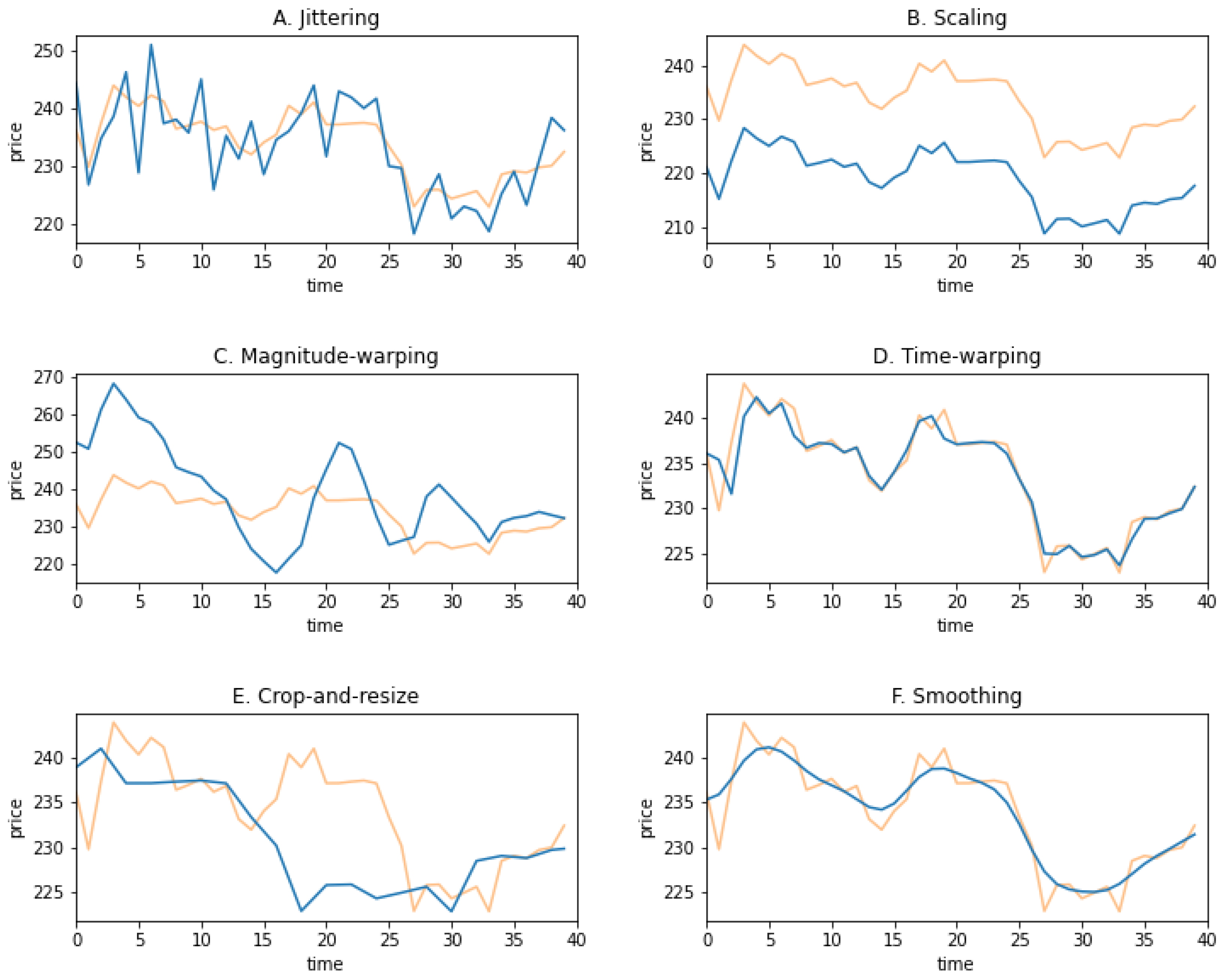
The performance of various data augmentation methods for time series have been investigated in some works [25,27,38,44], but not all make much sense for financial time series data. Therefore, we selected six different methods that are both commonly used and reasonable for our data. An example of the six augmentations is shown in Figure 5.
Jittering is to apply different noise to each data point. To implement it, we add to each window of time series a window-length vector ϵ with random values independently sampled from a normal distribution N ( 0 , σ 2 ) . The default value of standard deviation σ is set to 5. This yields to
X ˜ = X + ϵ , ϵ = [ ϵ 1 , ϵ 2 , , ϵ T ] , ϵ i N ( 0 , σ 2 )
where X represents the original window of data, and X ˜ represents the augmented data.
Scaling can be considered as multiplying each window by a factor λ , which is the absolute value of a random number sampled from a normal distribution N ( 1 , σ 2 ) . We set 0.6 as the default value of the standard deviation σ . This can be written as:
X ˜ = λ X , λ N ( 0 , σ 2 )
where X represents the original window of data and X ˜ the augmented data.
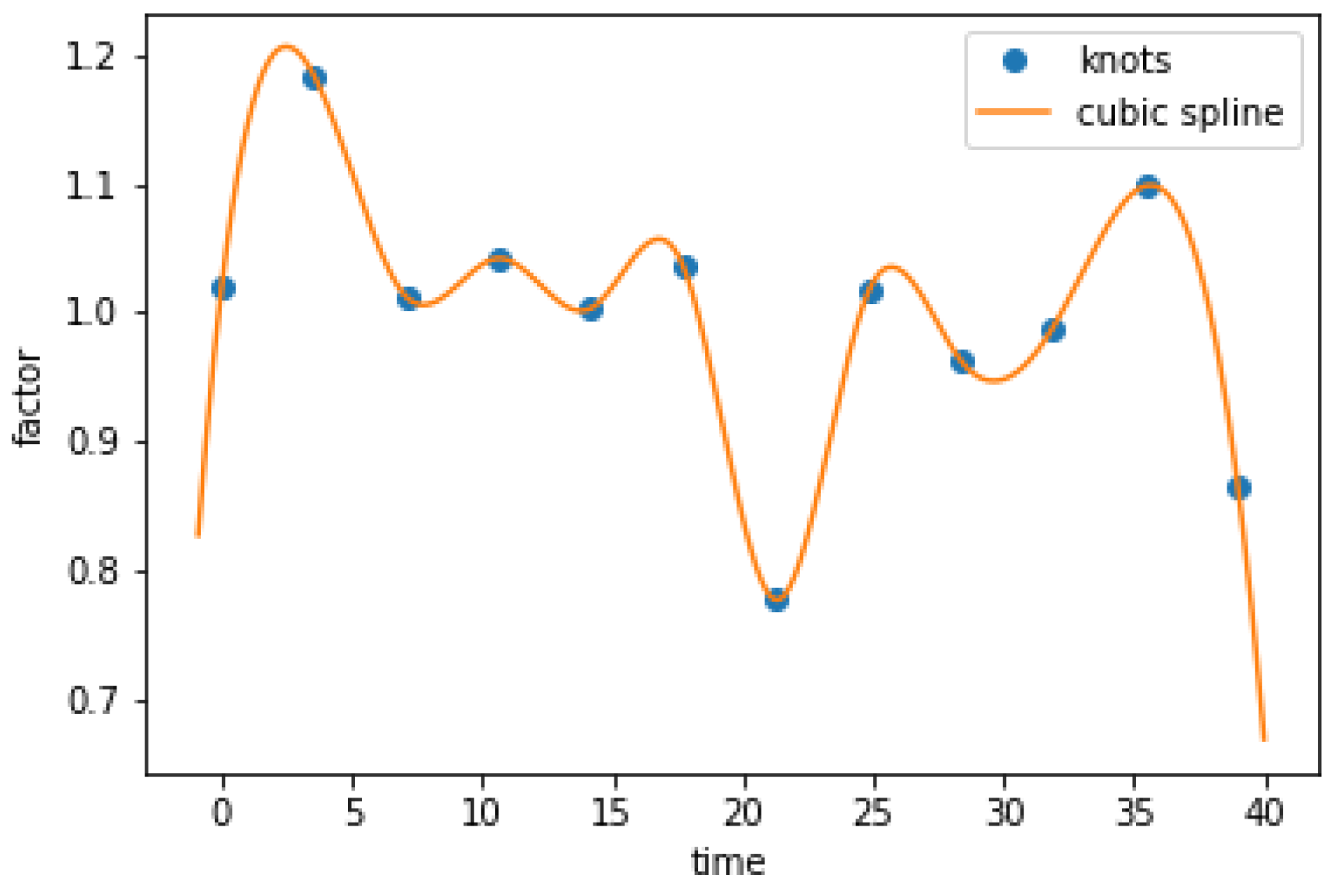
Magnitude-warping also scales data along the y-axis, but instead of applying a consistent factor, it multiplies different factors to different data points in a window. In addition, magnitude-warping requires the factors to be smoothly-varying. Specifically, we take k + 2 time points { 0 , ( T 1 ) / ( k + 1 ) , 2 ( T 1 ) / ( k + 1 ) , 3 ( T 1 ) / ( k + 1 ) , , k ( T 1 ) / ( k + 1 ) , T 1 } to divide the window of length T into k + 1 equal parts, and randomly draw k + 2 values { y 0 , y 1 , , y k , y k + 1 } from a normal distribution N ( 1 , σ 2 ) . With the k + 2 knots { ( i T / ( k + 1 ) , y i ) | i = 0 , 1 , , k + 1 } , a cubic spline can be fitted, as shown in Figure 6. The scaling factor corresponding to each time point can be obtained from the curve, and then we multiply the data by the factors. The whole process can be expressed as
X ˜ = λ X , λ = [ S ( 0 ) , S ( 1 ) , S ( 2 ) , , S ( T 1 ) ] R T
where X represents the original window of data, X ˜ the augmented data, S is the cubic spline. The default value of k is set to 10, and σ is set to 0.6.
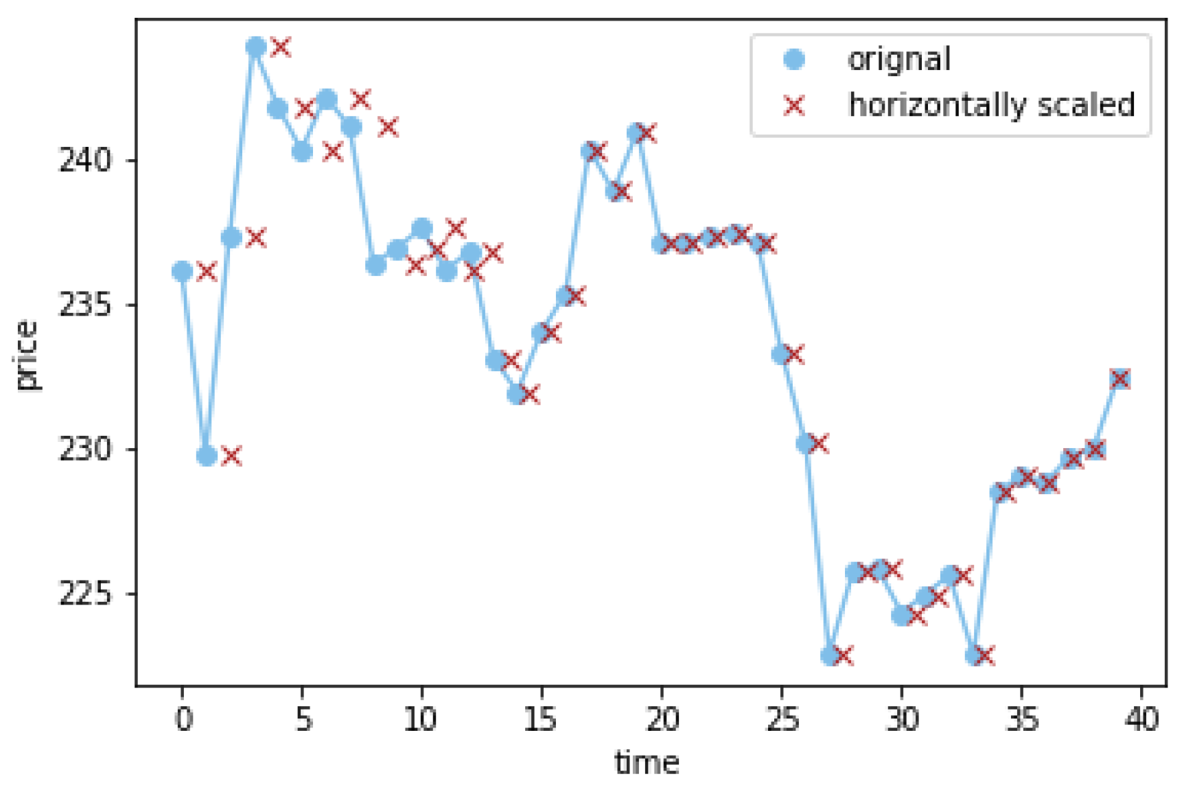
Time-warping is similar to magnitude-warping, but it scales data points along the time direction (x-axis). Specifically, we first generate a vector of factors λ = [ λ 0 , λ 1 , , λ T 1 ] in the same way as for magnitude-warping, then calculate the scaled cumulative sums of factors and obtain a vector λ = [ s λ 0 , s ( λ 0 + λ 1 ) , s ( λ 0 + λ 1 + λ 2 ) , , s ( λ 0 + λ 1 + + λ T 1 ) ] , where s = ( T 1 ) / ( λ 0 + λ 1 + + λ T 1 ) . By using λ (as timestamps) and original prices, new (horizontally scaled) data points can be generated, as shown in red in Figure 7. The final augmented prices are evaluated by applying linear interpolation at the original timestamps [ 0 , 1 , , T 1 ] . The introduced procedure is formulated as:
X ˜ = [ L ( 0 ) , L ( 1 ) , , L ( T 1 ) ] , L ( i ) = x i + ( i λ i ) x i + 1 x i λ i + 1 λ i , i = 0 , 1 , , T 2 , λ = [ λ 0 , λ 1 , , λ T 1 ]
where X ˜ represents the augmented data, x i is the original data of time i of the window, and L indicates the linear interpolation function formed by the scaled timestamps λ and the original data X = [ x 0 , x 1 , , x T 1 ] .
Crop-and-resize method cuts the original window to a shorter one and then makes it as long as before by interpolating new data points in it. To implement this, we first linearly interpolate between every pair of adjacent data points in the original window with length T, resulting in T 1 intermediate values and a new window with length 2 T 1 . Then we randomly select a sub-sequence with length T from the new window, and use it as the augmented data. This yields to
X ˜ = [ w i , w i + 1 , , w i + T 1 ] , i U ( 0 , T 1 ) w j = x j 2 if j is even 1 2 ( x j 1 + x j ) if j is odd , j = 0 , 1 , 2 , , 2 T 2
where X ˜ represents the augmented data, x i is the original data of time i of the window, and w i indicates the ith data points in the new window.
Smoothing is a method to remove noise and shows trends in the data. For each point in a window, we calculate the Gaussian kernel function values of it and its −2/+2 neighbors, and then take the weighted average of those data points. The process can be described by
X ˜ = [ z 0 , z 1 , , z T 1 ] , z i = r 2 x i 2 + r 1 x i 1 + r 0 x i + r 1 x i + 1 + r 2 x i + 2 , r j = pdf ( j ) pdf ( 0 ) + 2 pdf ( 1 ) + 2 pdf ( 2 ) , pdf ( j ) = 1 2 π σ 2 exp ( 1 2 σ 2 j 2 ) , σ U ( 1 , 2 )
where X ˜ represents the augmented data, x i is the original data of time i of the window. When calculating z’s, if there are not enough neighbors at left (or right), then we extend the input by replicating the existing leftmost (or rightmost) neighbor.

4. Experiments

In this section, we provide the details of data collection and models implementation and also evaluate our proposed model on Bitcoin bubble forecasting, and compare its performance with other machine learning and deep learning models.

4.1. Data

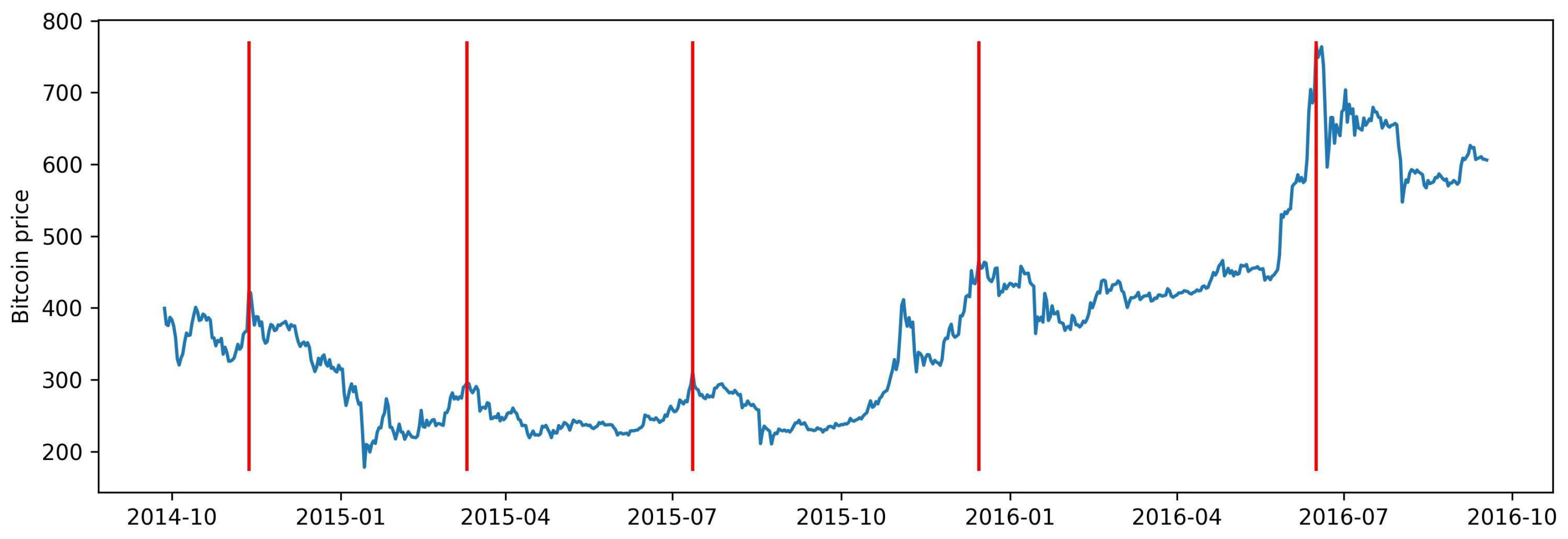
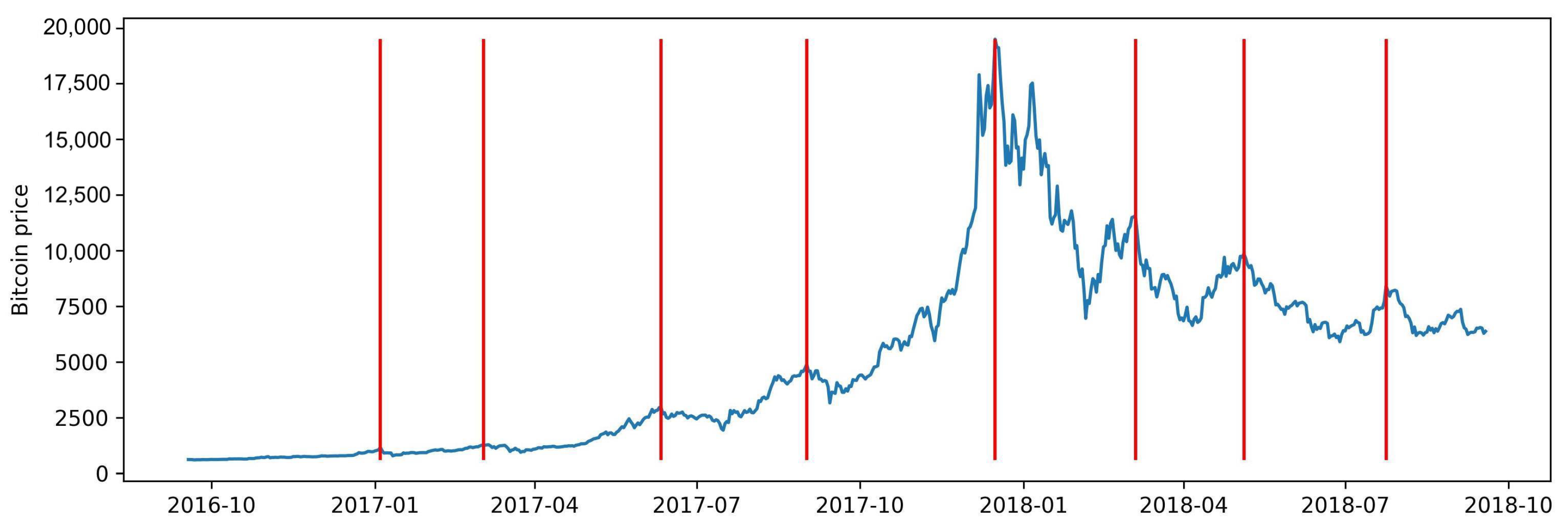
The data contains Bitcoin daily closing prices covering the period from 17 September 2014 to 17 September 2022 totally including 2923 time points, downloaded from Yahoo Finance. The target labels of drawdowns are determined by applying the Epsilon Drawdown Method with the expression ϵ = ϵ 0 σ ( ω ) , where ϵ 0 controls the number of standard deviations up to which counter-movements are tolerated, and ω determines the time scale on which the standard deviation is estimated. We perform a grid search over a predefined search space of ( ϵ 0 , w ) -pairs, scanning ϵ 0 with a step size of 0.1 from 0.1 to 5 and ω with a step size of 5 days from 10 to 60 days. Thus, there are in total 550 grid points. For each ( ϵ 0 , w ) -pair, a set of peak dates t p is recorded. After obtaining the 550 set of peak dates, we count the number of times that each date was identified as a peak day, and divide the count by 550 to obtain a fraction p t . By filtering peaks with p t > 0.65 and drop percentage > 20%, we obtain a total of 21 peaks, summarized in Table 2. The bitcoin historical prices of the whole selected period are visualized by the Figure A1,Figure A2,Figure A3 and Figure A4 in Appendix A.
We set the size of each window T = 30 and the prediction horizon M = 14 , and split the data by time, forming the training sets (80%) and the test sets (20%). The details of the two sets are listed in Table 3.

4.2. Contrastive Model Setup

For our experiments, we use the TensorFlow [45] deep learning framework. During the training of the CL models, we employ a sliding window with size of 30 and a moving step of 5. This yields 460 windows for training the CL encoder, which can be denoted as { X i } i { 1 , 6 , 11 , , 2296 } , where X i = [ x i , , x i + 30 1 ] . The dimension of the output space of projection head is specified at c o d e _ s i z e = 12 . The training process is done by using a batch-size of 16, 200 epochs and the ADAM optimizer [46] with learning rate of 1 × 10 4 . For contrastive loss calculating, the temperature parameter τ is set to 0.1. The downstream classifier is a linear layer with the sigmoid activation function, taking the representations extracted from CL encoder as input. To train the classifier, all windows in the training set are input, with batch of 32,200 epochs and class weights of {0:0.2, 1:0.8}. Model are trained 5 times with different random seed, and the averaged evaluation metrics are calculated. Hardware configuration: CPU of 2.6 GHz 6-Core Intel Core i7, RAM of 16 GB.
During the experiments, we calculate several metrics to evaluate the performance of models on the binary classification task; these are the following:
Balanced Accuracy: The balanced accuracy (BA) metric is the average of sensitivity and specificity. It can be written as:
BA = 1 2 ( sensitivity + specificity )
It is a performance metric that takes into equal consideration the accuracy obtained by the evaluated model in the both the majority class and minority class.
F2-score: F score measures the accuracy of a model using recall and precision. F2-score weights recall higher than precision, which is suitable for the situation where the tolerance for false negative samples is low. It is defined as:
F 2 = ( 1 + 2 2 ) precision · recall 2 2 · precision + recall
G-mean: The geometric mean (GM) is the product of sensitivity and specificity. It measures the balance between classification performances on the majority and minority class. It holds:
GM = sensitivity · specificity
Under this metric, poor performance in prediction of the positive cases will lead to a low G-mean value, even if the negative cases are correctly classified by the evaluated algorithm.
FM: The Fowlkes–Mallows (FM) index is the product of precision and recall. It measures the similarity between the predicted clustering and the true clustering. The value range of FM is [0,1], and the higher value means the better classification.

4.3. Baseline Models

The proposed contrastive model is compared with the following three categories of models:
  • Machine learning models include Random Forests (RF) [47], Support Vector Machine (SVM) [48], Gradient Boosting Machine [49] and XGBoost [50]. We used scikit-learn and XGBoost Python libraries to implement these models. Models are trained by using the extracted features from each window, instead of raw time series sequence data. Specifically, for each window, the average/standard deviation (std) of daily price ( p i )/return ( r i = ( p i p i 1 ) / p i 1 )/volatility ( v i = std ( [ r i 9 , r i 8 , , r i 1 , r i ] ) ) of the last 5 days, 10 days, 15 days,…, 30 days are calculated. In addition, tsfeatures Python library is applied to extract more advanced time series properties (see Table 4).
    In the training process, grid-search and 5-fold time-split cross-validation are employed. The configuration parameters of grid-search for each classification model are shown in Table 5.
  • Deep learning models contain LSTM [51] and the same TCN architecture used for contrastive learning but trained in a fully supervised manner. We used Both baseline models take the same input as the downstream classifier of the proposed contrastive learning framework. The LSTM model have two layers of a LSTM-ReLU-BatchNorm combination, followed by the projection head as CL and a dense layer with sigmoid activation function. For the TCN baseline model, two stacks of TCN followed by the projection head and a dense layer classifier are trained to directly predict the two desired classes for windows. We use batch of 32,200 epochs and class weights of {0:0.2, 1:0.8} to train the two DL models. Python library Tensorflow is also employed to implement the models.
  • Contrastive learning model uses the same architecture of the proposed framework but replacing the TCN encoder to an LSTM, which is consist of two layers of a LSTM-ReLU-BatchNorm combination. We denote this competitor as CL-LSTM. Similarly, the encoder is trained in self-supervised manner, using the same input and same experimental setup with CL-TCN.
  • LPPLS Confidence Indicator is constructed by using the shrinking windows whose length is decreased from 360 days to 30 days. For each fixed end point t 2 , we shift start point t 1 in steps of 30 days, hence totally 12 of fittings are generated. To estimate parameters and filter fittings, we apply the following search space and filtering condition in Table 6.

4.4. Augmentation Comparison and Analysis

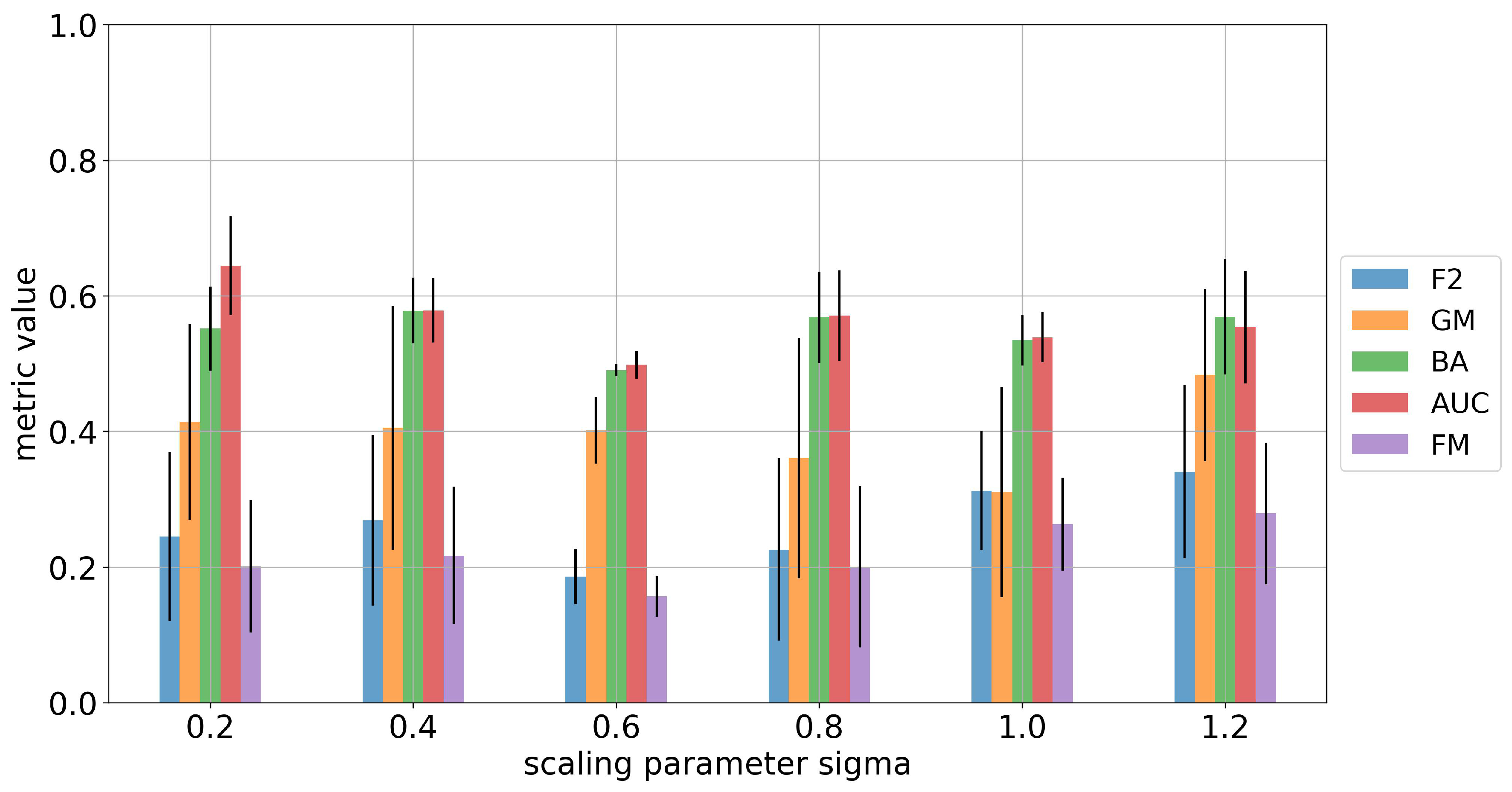
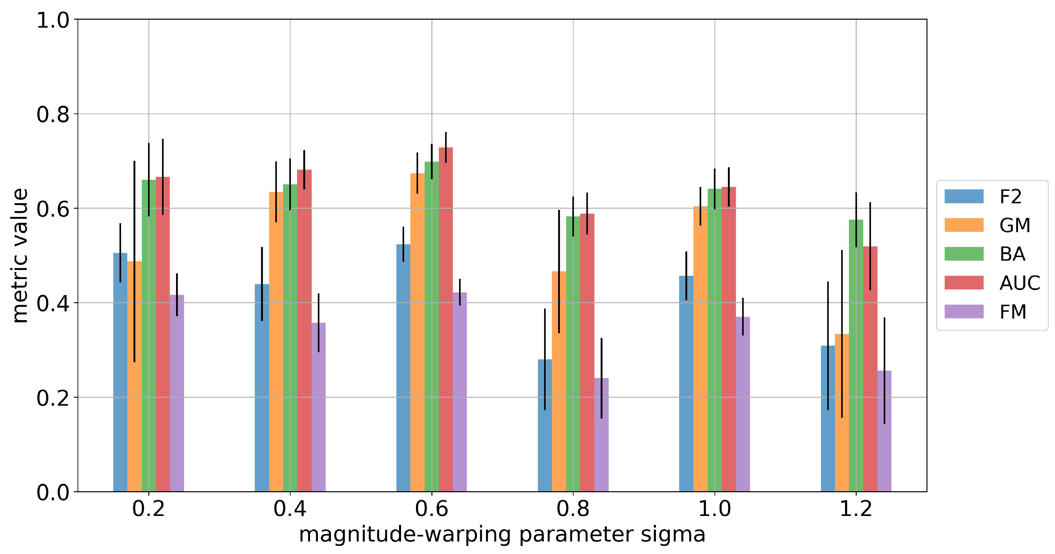
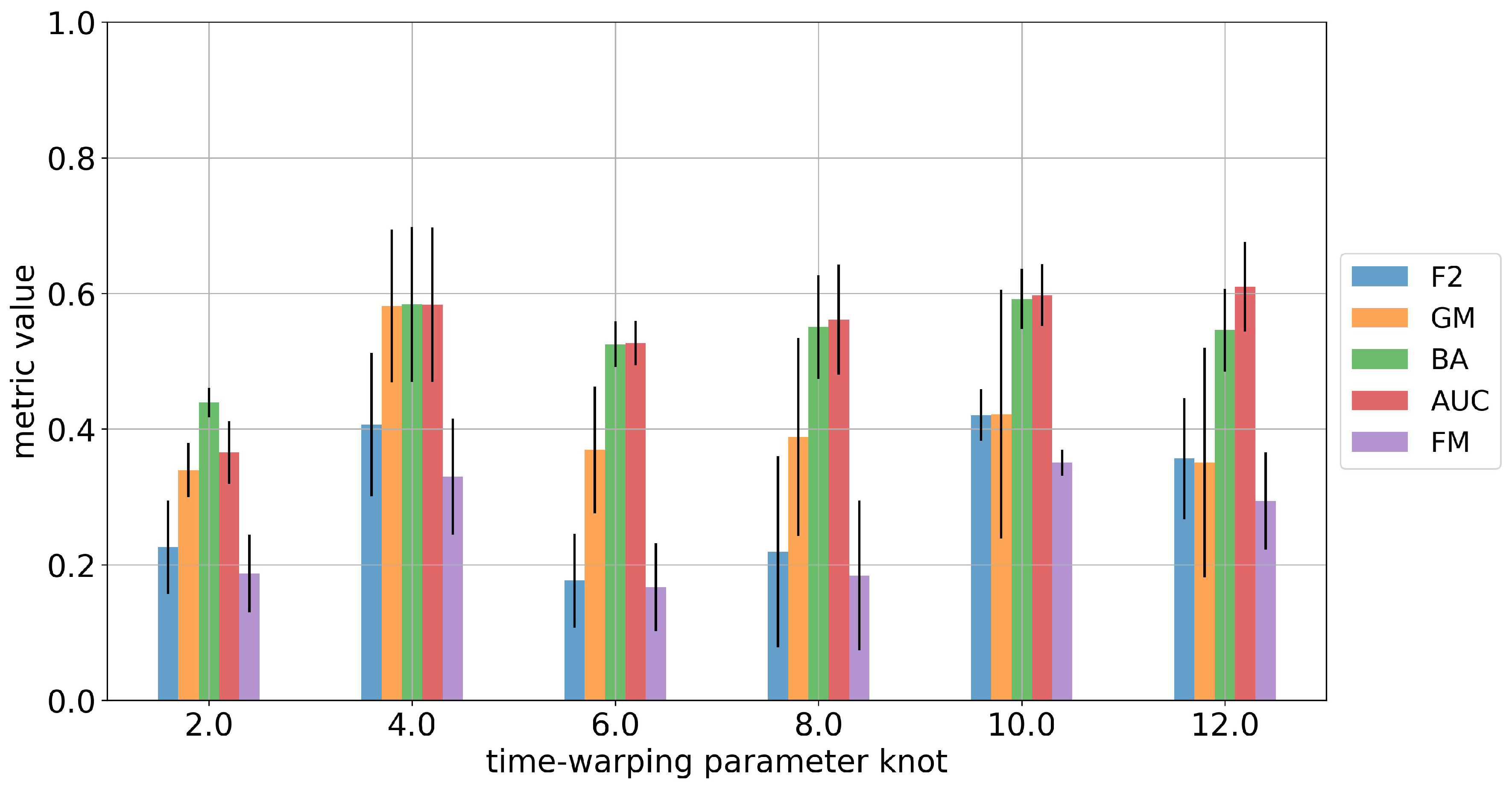
First, to investigate how the values of augmentation parameters would affect the model performance, we conduct a hyperparameter sweep by testing over a parameter space on four augmentation approaches—jittering, scaling, magnitude-warping and time-warping. For jittering and scaling, we test their scale parameters σ , while for magnitude-warping and time-warping, both knot parameter k and scale parameter σ are investigated. The results are visualized by bar plots, shown in Figure A5, Figure A6, Figure A7, Figure A8, Figure A9 and Figure A10 in Appendix A. We find that the impact of most augmentation approaches appears to be relatively affected by adjusting the parameters in a certain range. Therefore, in the following experiments, each augmentation method is applied with the parameters that have the best performance across all the evaluation metrics. Specifically, for jittering, σ = 1.0 ; for scaling, σ = 1.2 ; for time-warping σ = 0.6 , k n o t = 8 , and magnitude-warping σ = 0.6 , k n o t = 10 .
Then, we conduct an one-head experiment—throughout the whole training loop, we apply one fixed augmentation on one head while the other head executes an identity function, and compare the model performance with different augmentation in order to identify the most promising augmentations from the introduced function pool while excluding the least promising ones. The results are summarized via the evaluation metrics given in Table 7.
As a result, augmentations like crop-and-resize and smoothing can be discarded, because they perform worse than the baseline under all the metrics as they appear to hinder rather than to improve the training process. Scaling has worse performance when evaluated by G-mean, and therefore we will not consider it in the later experiments either. In contrast, time-warping, jittering and magnitude-warping appear to be the front-runners, yielding significant increases in all measured metrics compared to the baseline without augmentation.
Furthermore, by only considering the three best methods in the one-head experiment, we test the effect of two-head augmentation strategy. Specifically, we select two augmentation methods, and use one on the first head and the other on the second head, with default values of augmentation parameters. The results are shown in Table 8. We find that only the combination of jittering and magnitude-warping achieves significant increases of all evaluation metrics when compared to applying no augmentation at all; while the other two combinations do not show strong effect on improving the model performance. Compared with the results from the one-head strategy (Table 7), it is obvious that jittering can be improved by collaborating with other augmentations, but both time-warping and magnitude-warping perform worse in combination with other methods than alone.
To verify if using only one augmented head is better than applying augmentations on two head, we run experiments for augmentation combinations using by the three front-runners. Specifically, here we apply one method followed by another on the first head and identity on the second head. The performances of different combinations are summarized in Table 9. It shows that the combination of time-warping and magnitude-warping far outperforms not only the baseline, but other combinations as well. By comparing with the two-head experiment (Table 8), we find that time-warping tends to have greater performance in the one-head setting.

4.5. Fine-Tuning and Sensitivity Analysis

To investigate the sensitivity of the proposed model, we conduct additional experiments by adjusting the following parameters:
  • Window size is the length of original time series sequence input. We think that different window sizes contain different information, so it should be large enough to contain the most useful information for prediction but not too long to make the model hard to catch the key properties of the sequence. We select window sizes of 30, 90, 180 and 360 days for the experiment.
  • Batch size specifies the number of positive pairs (K) of augmented windows that are processed before the model is updated, so in our case there are 2 K training samples in each batch. In the experiment, the batch size is chosen to be 16, 32, 64 and 128.
  • Code size indicates the length of the embedding vector (representations) that is extracted from the encoder network. The code size is tested to range between 8 and 24.
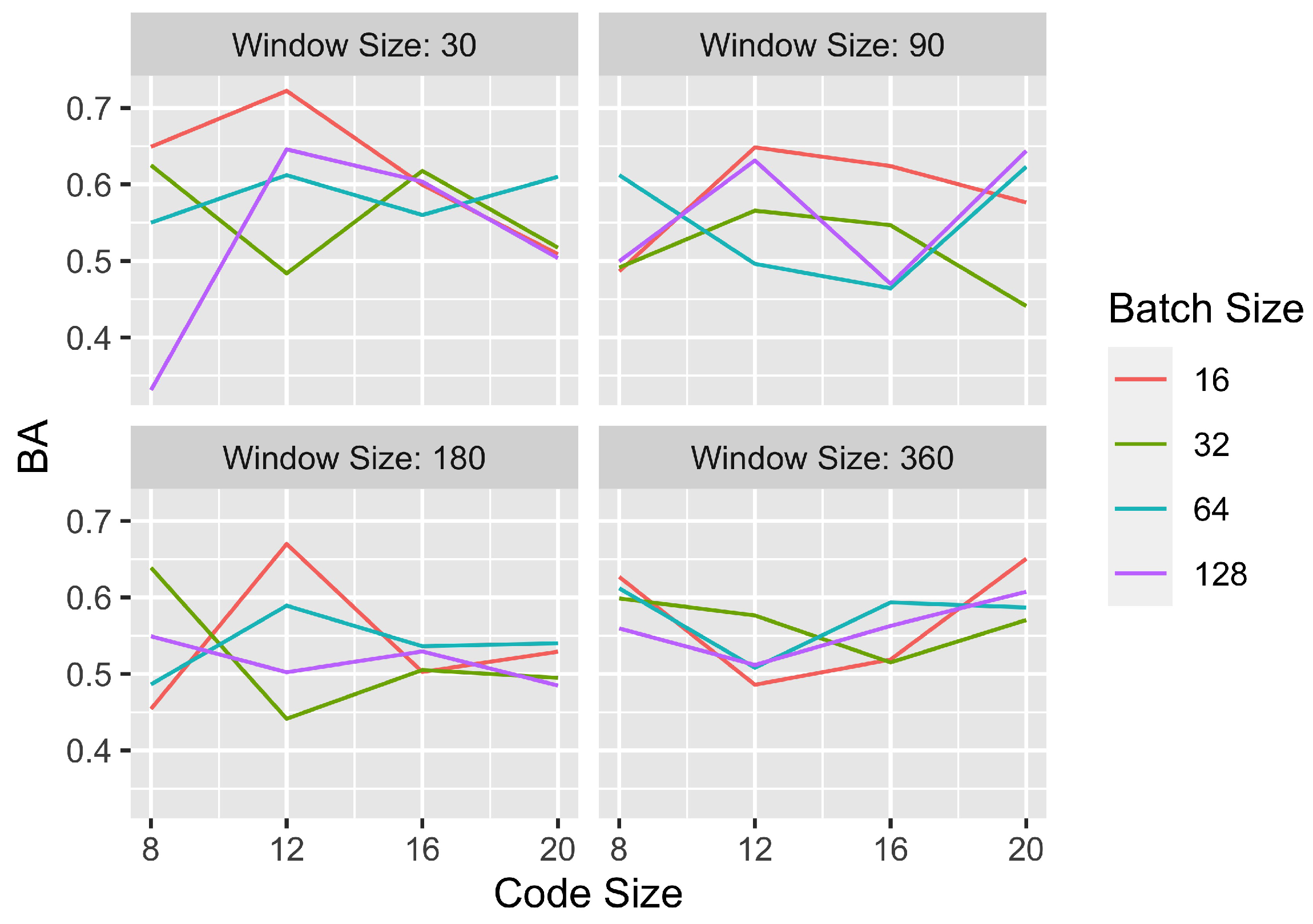
Figure 8 visualizes the results of comparing the performance of the proposed framework (with respect to BA) across the different parameter settings. It demonstrates that averaged over the code size and batch size, the model has relatively same performance with different window size, but the model tends to have slightly variable performance when training with smaller size of windows. It is expected that 30 days is an effective length of window, and windows too long may render it difficult for the model to extract more predictive information.
For the batch size with respect to the set of { 16 , 32 , 64 , 128 } , we find that the proposed model has robust performance, when taking average across the code size and window size (Figure 9). With window size 30 and 90, the models with batch 16 obviously outperform the ones with other batch sizes. We believe this situation occurs because small batch size makes it less likely that a sample will be similar to other samples in the same batch, which enables the model to better distinguish negative pair of samples. But as the window size increases, the probability of a negative pair of samples being very similar decreases, so changing batch size does not have a large impact on the model performance.
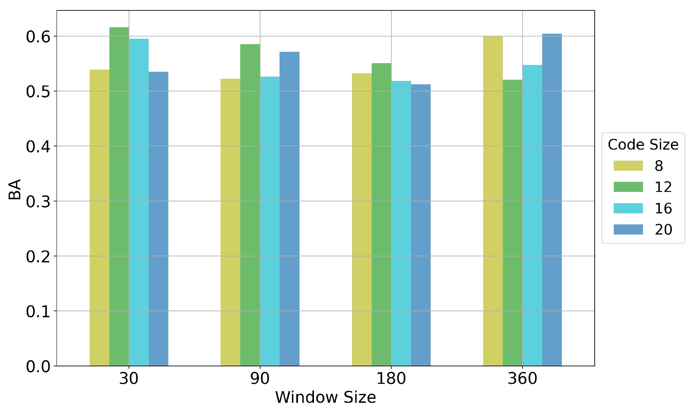
As shown in Figure 10, at the window size of 30, 90 and 180, the model performance, averaged over the batch size, has the best BA at a code size of 12, while for longest window of 360, a larger code size is needed to contain enough information in their representations.

4.6. Baseline Comparison

To demonstrate the effectiveness of our model, we compare its performance to the seven baseline ML/DL models. Table 10 gives an overview of the comparison results. For each measurement, the highest value is highlighted in bold, the second highest one is marked by underline, and the third highest is presented in italic.
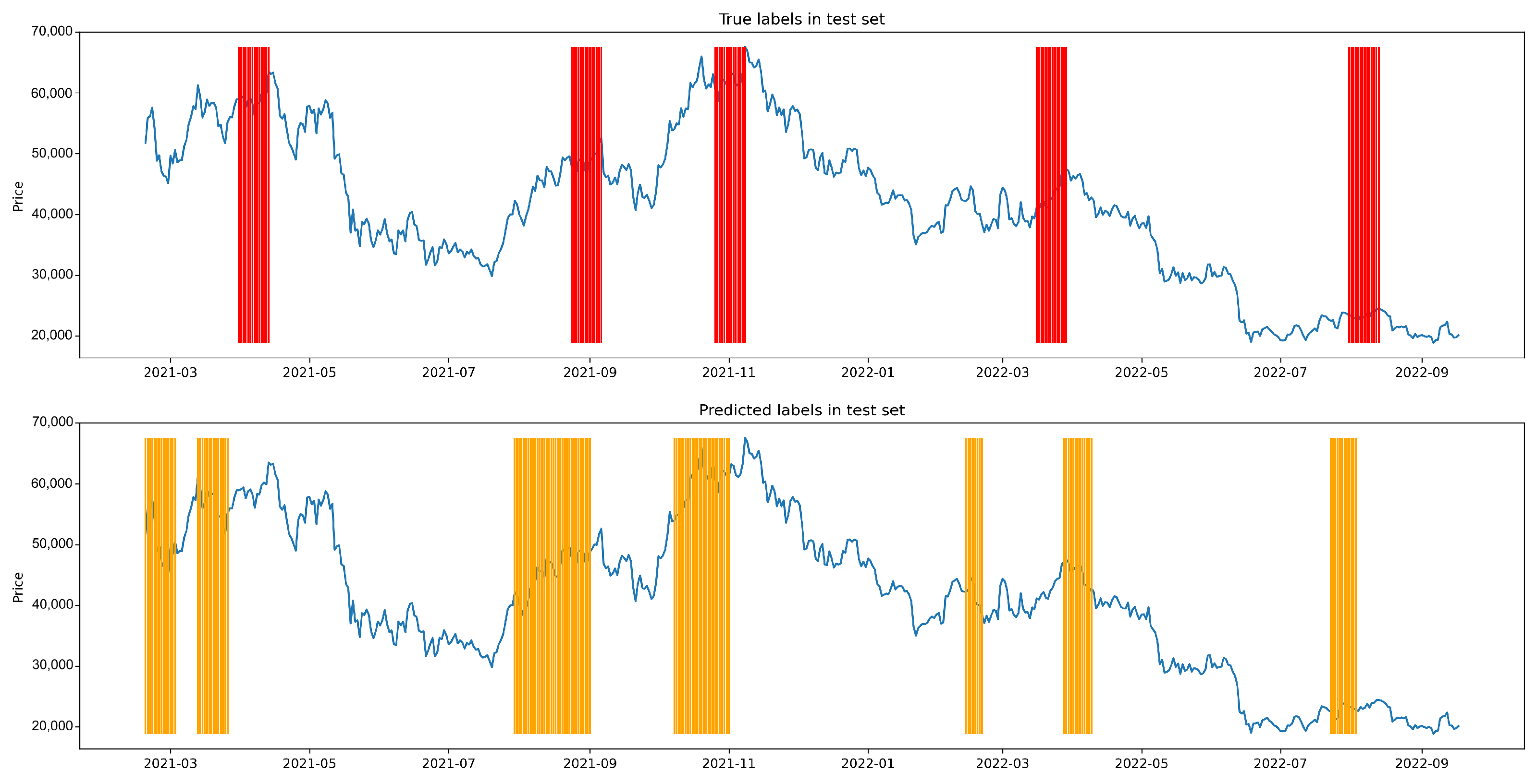
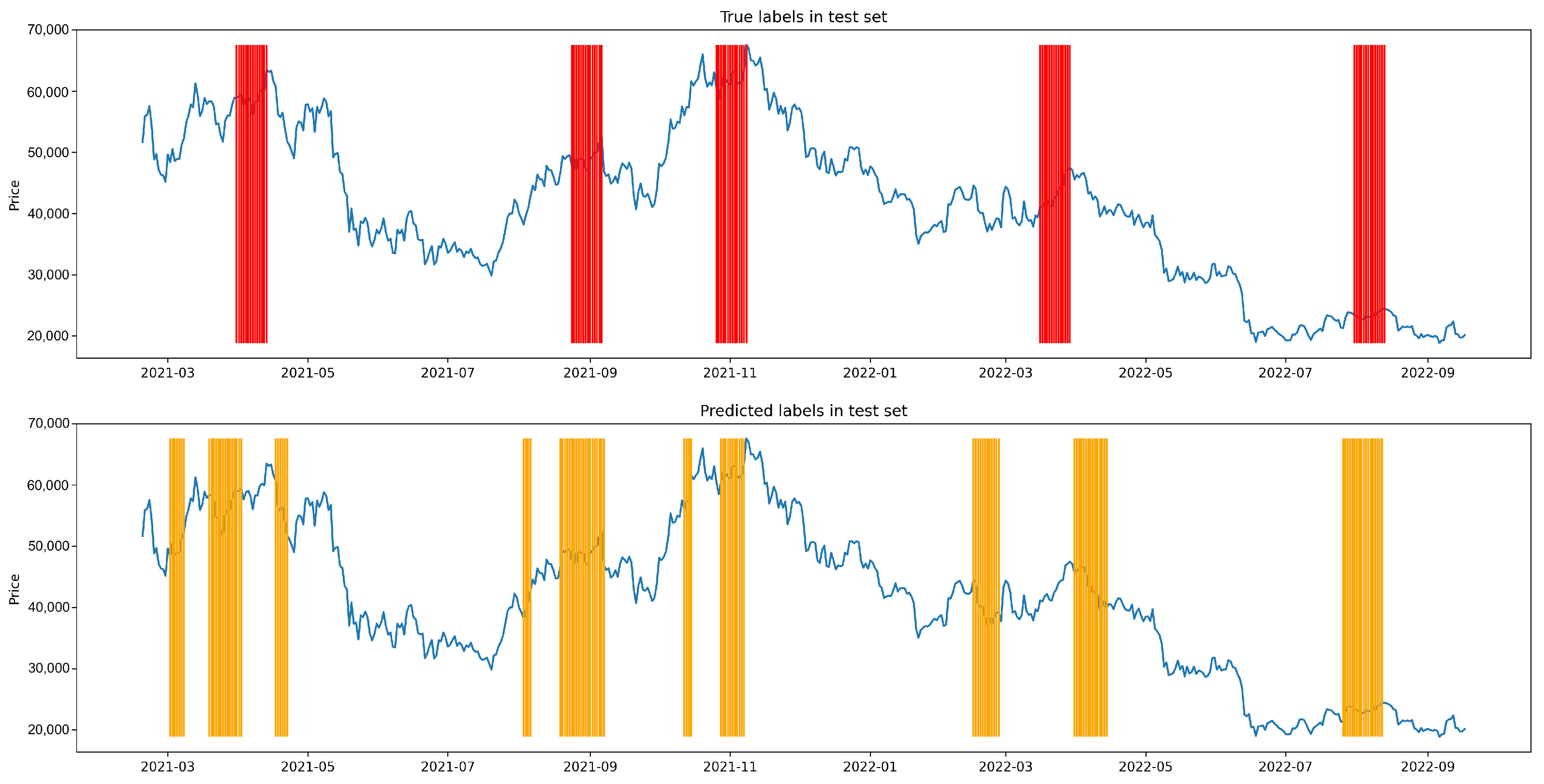
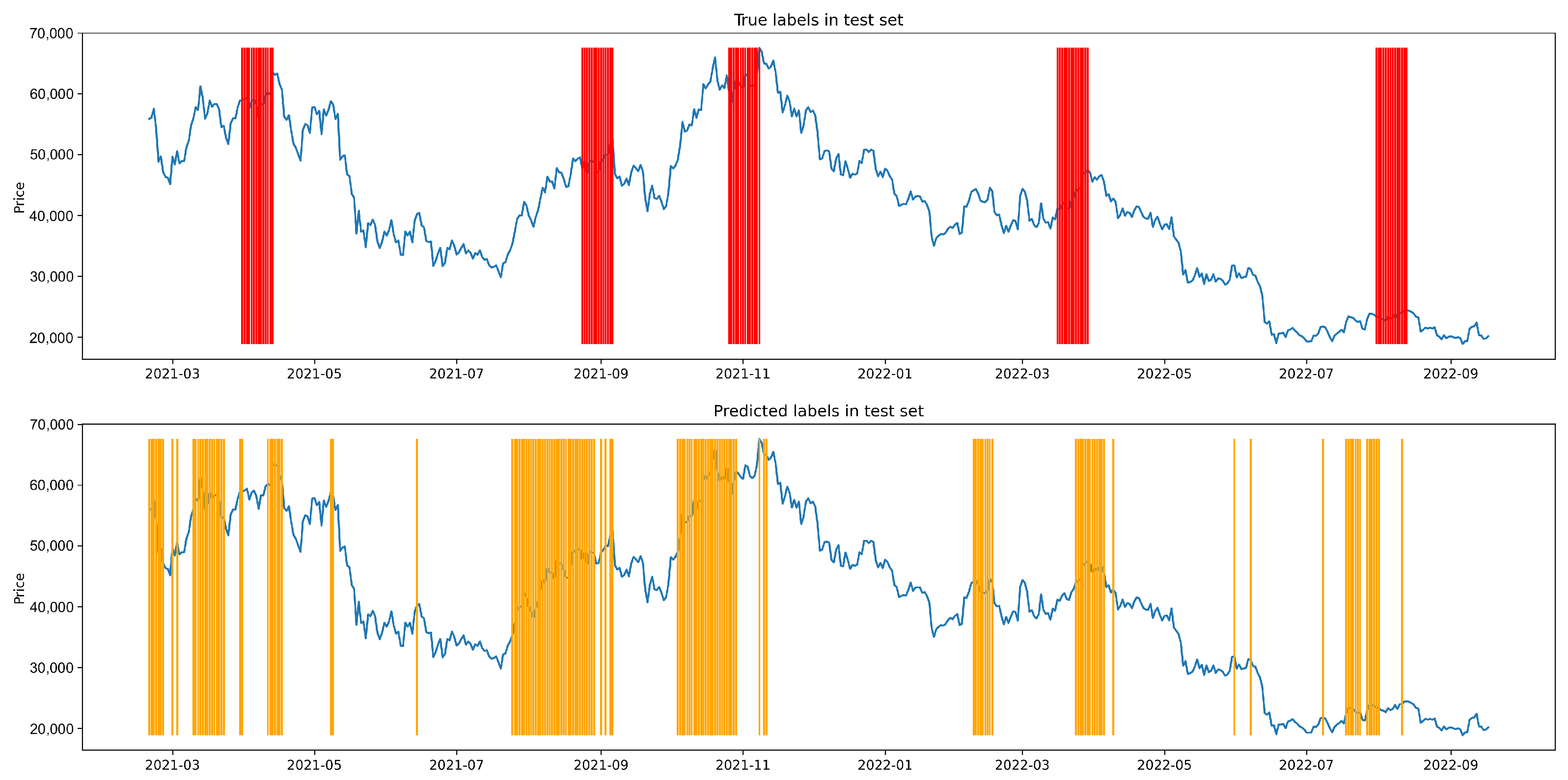
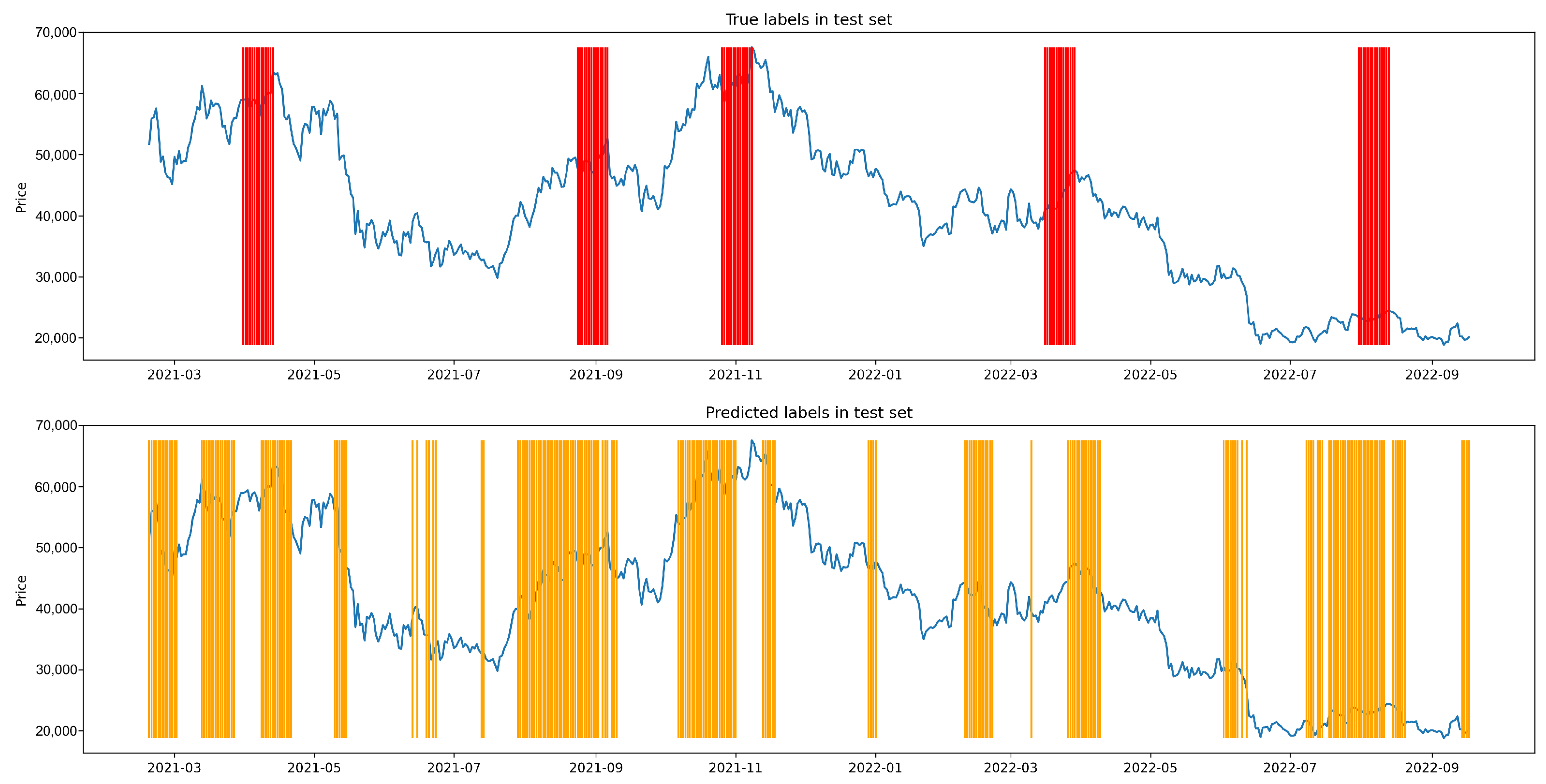
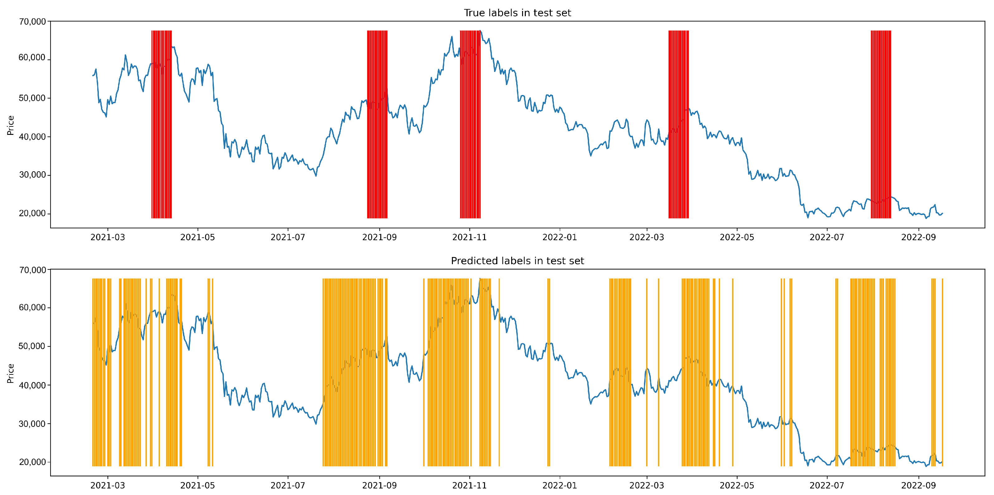
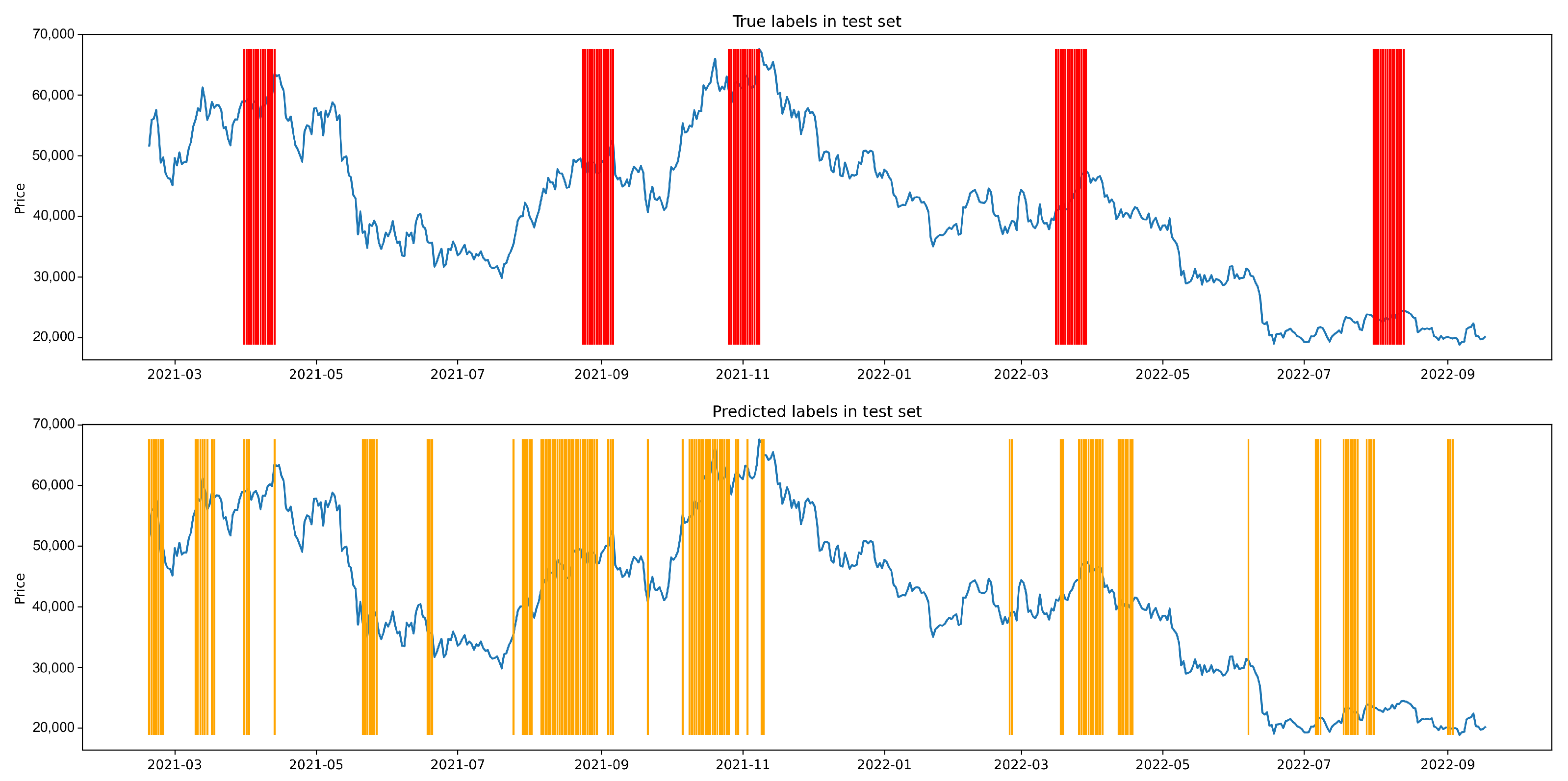
We can see that our proposed framework could achieve the best performance over all the selected evaluation metrics, higher BA and GM indicates that our proposed framework has better accuracy on classifying both majority class (non-bubble periods) and minority class (bubble periods), while the larger F2-score and FM index implies that it is less likely to incorrectly predicts bubbles as non-bubbles. In addition, TCN and XGB, the second best and the third best models, outperform others by an obvious margin. The visualization of eight models prediction results on test set are shown in Appendix A Figure A11, Figure A12, Figure A13, Figure A14, Figure A15, Figure A16, Figure A17 and Figure A18.
Through not only the comparison between LSTM and TCN but also the comparison between CL-LSTM and CL-TCN, it is shown that TCN outperforms LSTM on extracting effective representations for time series. This result aligns with the conclusions make in works [39,40,41,42], so that it provides a strong support for our choice of TCN as the encoder rather than LSTM.
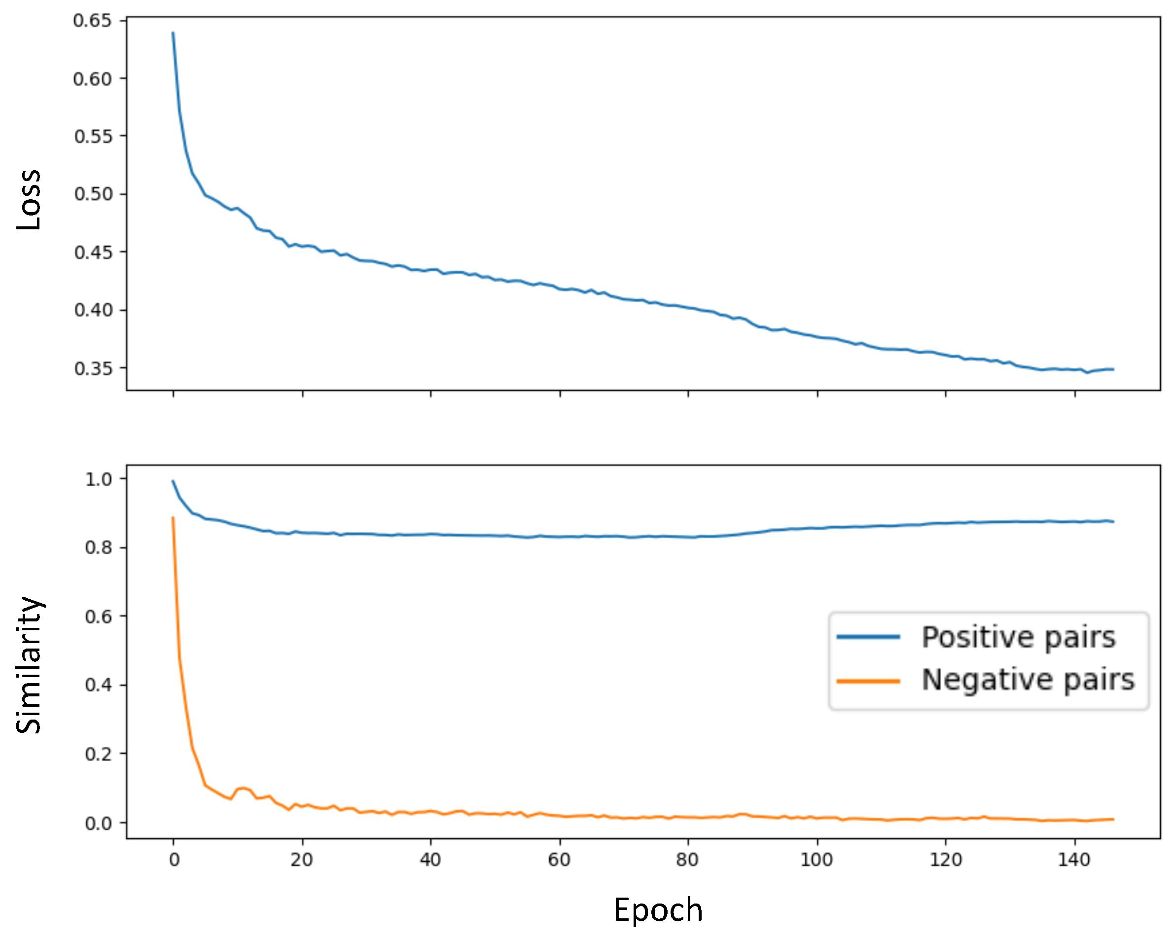
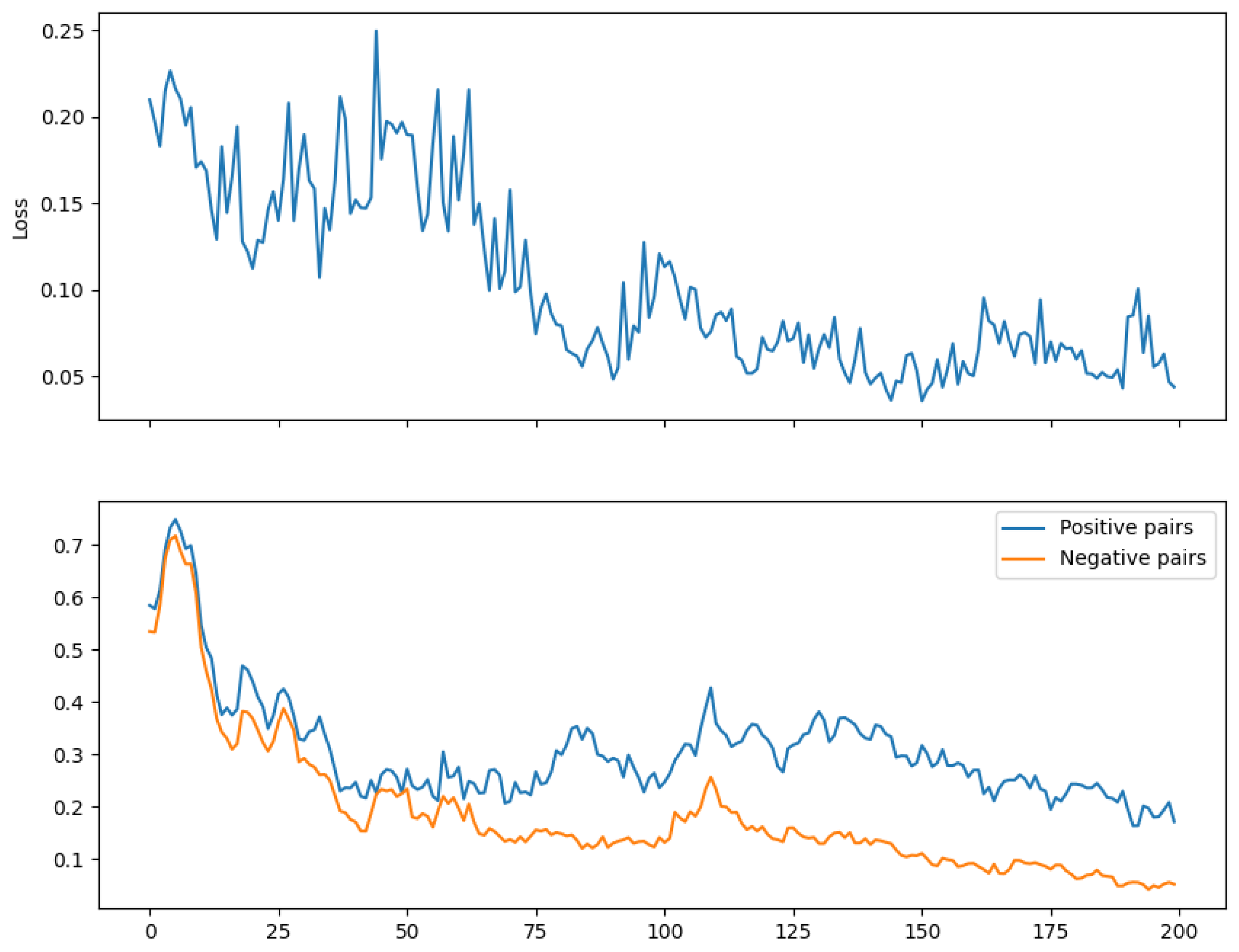
The pre-training loss and similarity trajectory of CL-TCN and CL-LSTM are shown in Figure 11 and Figure 12. We can find that TCN encoder learns to distinguish similar samples from different samples in very less epochs, and keeps making the similarity between positive pairs extremely high, while the similarity between negative pairs is near to zero. However, in the first 50 epochs, the epoch-wise averaged similarity for positive pairs is close tightly to that for negative pairs, which indicates that CL-LSTM has a difficulty in distinguishing samples. Although at the end, CL-LSTM make the similarity of negative pairs near to zero, the similarity for positive pair is too low.

4.7. Ensemble Model

Due to the inherently challenging nature of forecasting stock market crisis events on the global scale, it is well-expected that all postulated models are rather weak learners. Some may achieve better modeling performance under specific observed patterns, others under different ones, but we do not expect any single one to capture best all the existing latent patterns. Hence, exploiting forecast combinations that allow us to assign different weights to each of the obtained predictions is expected to boost the overall attainable predictive performance.
Specifically, ensemble modeling is the act of executing two or more related but distinct analytical models and then combining the results into a single score or spread. Empirically, ensembles tend to yield better results when there is a significant diversity among the models. For ML/DL models, we combine the three best performers (CL-TCN, TCN, XGB) together as a ensemble model in three ways—hard vote, soft vote with simple average, and soft vote with weighted average. Since the LPPLS indicator cannot be regarded as predicted probability, logistic regression is conducted by taking the indicator as a input feature. Also, to construct an ensemble CL that is more comparable to LPPLS indicator, we follow the construction logic of LPPLS indicator to implement a CL-indicator.
  • Hard Vote
    In hard voting (also known as majority voting), every individual classifier votes for a class, and the majority wins. The ensemble’s anticipated target label is, statistically speaking, the mode of the distribution of the labels’ individual predictions. In this case, the selected three base models generate binary predictions separately. If more than 2 models infer positive output then the ensemble model output is marked as positive, otherwise marked as negative.
  • Soft Vote (Simple Average and Weighted Average)
    In soft voting, every individual classifier provides a probability value that a specific data point belongs to a particular target class. A simple average strategy is firstly applied and converted to binary predictions for evaluation. For weighted average, the evaluation metric value of each base classifier is used to weight and then average the predictions. As multiple metrics are adopted in evaluation above (F2, GM, BA, FM), the weight can be calculated by looping through them. Different weighted average output can be generated, and consequently the final binary label by metric is gathered.
  • Logistic Regression
    Logistic regression is conducted by using the predicted probabilities of the 3 selected and the LPPLS indicator as 4 features to fit on the train set, then predict on the test set.
  • CL Indicator
    Same as constructing LPPLS indicator, we recursively train CL-TCN with shrinking window of 360 days to 30 days with a step size of 30 days, hence the 12 CL models are obtained. For each time point, we use 12 models to make prediction and then calculate the fraction of models that classify it as class 1.
The comparison of performance between ensemble models and CL-TCN are shown in Table 11. We can find that Simple Average Soft Vote outperforms other ensemble models and has comparable performance with CL-TCN. The logistic regression has a significant decrease for all the evaluation metrics.
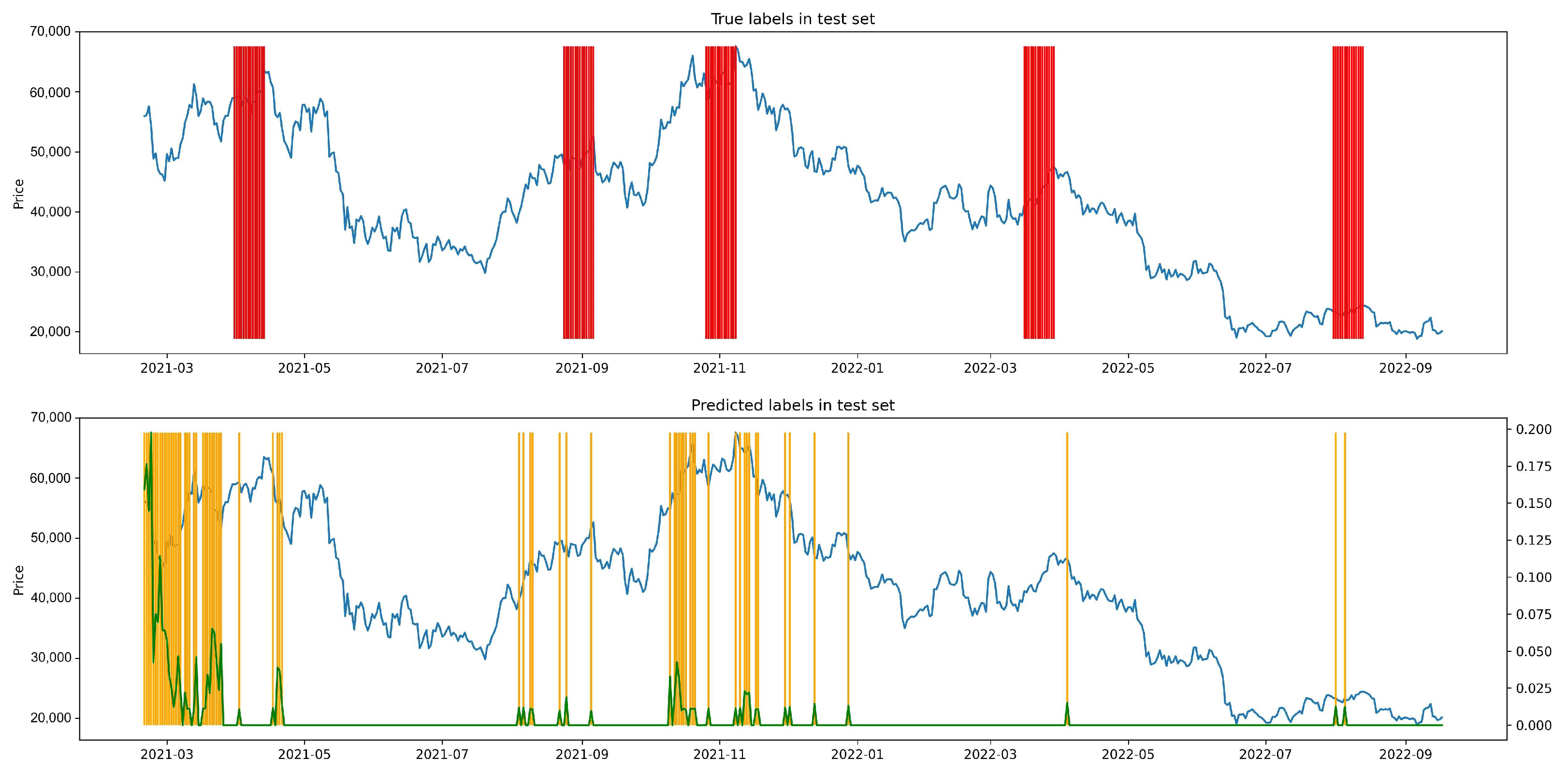
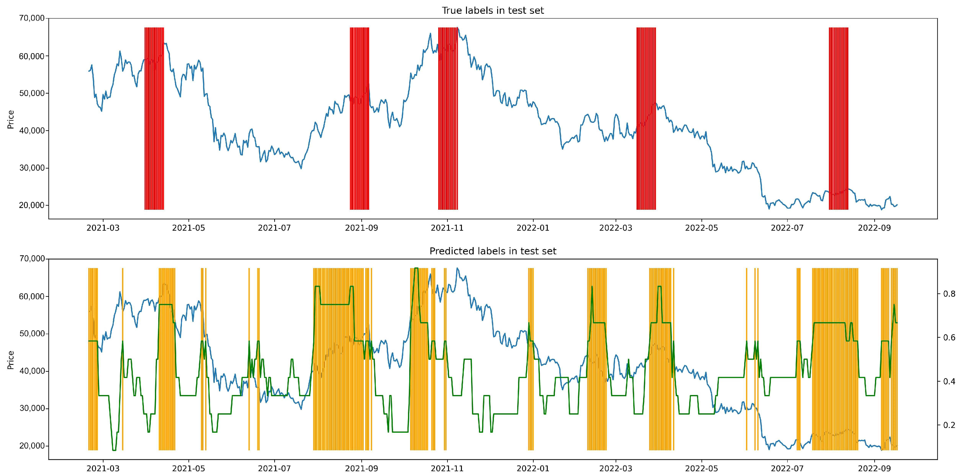
The comparison results of LPPLS-indicator and CL-indicator is summarized in Table 12 and visualized in Figure 13 and Figure 14.
From Figure 13 and Figure 14, we can see the indicators result (in green) on test set in the lower panel, and its corresponding y-axis is on the right side of the panel. It is obvious that the indicators of most time point are 0, so we set the threshold to 0 for converting it into binary classes. We find that LPPLS indicator makes alert for all the drawdowns on the test set and have not too much false positive result, although for some drawdowns it is very weak. Compared to CL-indicator, it makes long-time alert for every drawdowns, and also correctly predicted other small drawdowns that are not selected as true label.

5. Conclusions

In conclusion, our study introduces a contrastive learning-based classification framework for predicting financial bubbles and crashes, with a focus on Bitcoin price data. By leveraging the SimCLR and making modifications, we achieve improvements in prediction performance compared to various ML/DL models. Moreover, we introduce a CL-indicator and make comparison between it with LPPLS-indicator, which is unprecedented, to the best of our knowledge. Our results demonstrate the effectiveness of CL in extracting meaningful representations from time series data, paving the way for better understanding and forecasting of financial market dynamics.
The success of our approach suggests its potential applicability to other financial indicators and markets, opening up opportunities for further research in diverse areas such as stock price prediction, regime change detection, and price movement forecasting. Additionally, the scalability of our framework allows for the incorporation of macroeconomic variables, enhancing its predictive power and practical utility in real-world applications.
In future work, we plan to explore the integration of additional features and advanced data augmentation techniques to further improve the performance of our model. Moreover, we aim to extend our analysis to other time series datasets and tasks, while also exploring the use of more sophisticated classifiers to enhance the robustness and generalizability of our framework. Overall, our study contributes to the growing body of research on predictive analytics in finance and highlights the potential of CL as a valuable tool for financial forecasting and risk management.

Author Contributions

Conceptualization, Z.L., M.S. and W.Z.; Methodology, Z.L. and M.S.; Software, Z.L.; Validation, Z.L.; Formal analysis, Z.L.; Investigation, Z.L. and M.S.; Resources, M.S. and W.Z.; Data curation, Z.L.; Writing—original draft, Z.L.; Writing—review & editing, Z.L., M.S. and W.Z.; Visualization, Z.L.; Supervision, W.Z. All authors have read and agreed to the published version of the manuscript.

Funding

This research received no external funding.

Institutional Review Board Statement

Not applicable.

Informed Consent Statement

Not applicable.

Data Availability Statement

Bitcoin daily closing prices were downloaded from https://finance.yahoo.com/.

Conflicts of Interest

The authors declare no conflicts of interest.

Appendix A

Appendix A.1. Features from Tsfeatures

Autocorrelation function (ACF) and partial autocorrelation function (PACF) features are used to measure the correlation among the values in each window. Feature acf_1 is the first autocorrelation coefficient. The features acf_10 is the sum of squares of the first ten autocorrelation coefficients. Moreover, autocorrelations of the changes provide a window without temporal changes (e.g., trend and seasonality). Thus, differentiating is first calculated to compute the differences between consecutive observations within a window, and then the ACF parameters are computed. Feature dacf_1 obtains the first autocorrelation coefficient from the differenced data. The features dacf_10 measures the sum of squares of the first ten autocorrelation coefficients from the differenced series. The first derivative of windows derives velocity of deformation. Additionally, d2acf_1 and d2acf_10 provide similar values corresponding to the twice-differenced series (i.e., the second-order differencing operation from the consecutive differences). In fact, the second derivative obtains the displacement acceleration in windows. Similarly, three features (see Table 4) are computed by the Partial Autocorrelation Function (PACF) of the first five partial autocorrelation coefficients, including pacf_5, dpacf_5, and d2pacf_5. The partial autocorrelation assesses the relationship of observations with shorter lags.
Seasonal and Trend Decomposition Using the LOESS (STL) method decomposes a time series window into a trend (i.e., trend-cycle), seasonal, and residual components. Trend shows the strength of a cyclic trend inside a window from 0 to 1. Spike represents the prevalence of spikiness in the remainder component of the STL decomposition. Linearity and curvature features estimate the linearity and curvature of the trend component by applied linear and orthogonal regressions, respectively. Features stl_1 and stl_10 represent the first autocorrelation coefficient and the sum of squares of the first ten autocorrelation coefficients of the remainder series, respectively.
Other features are extracted to develop further properties on deformation of windows. Nonlinearity determines the log of a ratio consisting of the sum of squared residuals from a nonlinear and linear autoregression by Teräsvirta’s nonlinearity test [52], respectively. The entropy metric measures the spectral density of a window, quantifying the complexity or the amount of regularity. Lumpiness and stability features measure the variance of the means and the variances on nonoverlapping windows, which provide information on how a window is free of trends, outliers, and shifts. Finally, the last three features, max_level_shift, max_var_shift, and max_kl_shift, denote the largest shifts in mean, variance, and Kullback–Leibler divergence of a window based on overlapping windows, respectively. These features may distinguish valuable structures regarding the window with jumps.

Appendix A.2. Figures

Figure A1. Identified bitcoin bubble peaks between 2014 and 2016.
Stats 07 00025 g0a1
Figure A2. Identified bitcoin bubble peaks between 2016 and 2018.
Stats 07 00025 g0a2
Figure A3. Identified bitcoin bubble peaks between 2018 and 2021.
Stats 07 00025 g0a3
Figure A4. Identified bitcoin bubble peaks between 2021 and 2022.
Stats 07 00025 g0a4
Figure A5. Effect of varying the scale parameter on jittering.
Stats 07 00025 g0a5
Figure A6. Effect of varying the scale parameter on scaling.
Stats 07 00025 g0a6
Figure A7. Effect of varying the scale parameter on magnitude-warping.
Stats 07 00025 g0a7
Figure A8. Effect of varying the knot parameter on magnitude-warping.
Stats 07 00025 g0a8
Figure A9. Effect of varying the scale parameter on time-warping.
Stats 07 00025 g0a9
Figure A10. Effect of varying the knot parameter on time-warping.
Stats 07 00025 g0a10
Figure A11. Visualization of prediction of CL-TCN on test set.
Stats 07 00025 g0a11
Figure A12. Visualization of prediction of TCN on test set.
Stats 07 00025 g0a12
Figure A13. Visualization of prediction of XGB on test set.
Stats 07 00025 g0a13
Figure A14. Visualization of prediction of GBM on test set.
Stats 07 00025 g0a14
Figure A15. Visualization of prediction of CL-LSTM on test set.
Stats 07 00025 g0a15
Figure A16. Visualization of prediction of RF on test set.
Stats 07 00025 g0a16
Figure A17. Visualization of prediction of LSTM on test set.
Stats 07 00025 g0a17
Figure A18. Visualization of prediction of SVM on test set.
Stats 07 00025 g0a18

Appendix A.3. Shuffle Experiment

For the original Bitcoin daily price time series, we randomly shuffle it to create 10 new time series sequences. Then, we apply the same Epsilon Drawdown Method and grid search setting introduced in Section 4.1 to obtain target labels for each new sequence. Under the same pre-processing steps and model configurations, we train our model, make prediction and get corresponding evaluation metrics. The results obtained with the original time series and those obtained with the shuffled time series are summarized below.
Table A1. Comparison of models performance between original Bitcoin daily price data and shuffled data.
F2GMBAFM
original0.54 ± 0.06 0.71 ± 0.04 0.72 ± 0.04 0.44 ± 0.04
shuffle0.31 ± 0.18 0.40 ± 0.18 0.47 ± 0.16 0.26 ± 0.14
Since our model relies on the assumption that the sequential order of observations contains valuable predictive information, the degradation in performance on shuffled data suggests that this assumption is valid. It highlights the complexity of the temporal dynamics underlying Bitcoin price movements, and indicates that simply shuffling the order of observations disrupts the underlying patterns and dependencies in the data, making it more challenging for our proposed framework to capture and exploit meaningful information for drawdown prediction.

Appendix A.4. Drawdowns in Bitcoin Hourly Price Data

To make more comprehensive comparison between our proposed framework and baseline models, we incorporate hourly prices of Bitcoin from 10 April 2022 10 a.m. UTC to 19 September 2023 11 p.m. UTC, which includes 12,401 time points. The target labels of drawdown are also generated by applying the Epsilon Drawdown Method, scanning ϵ 0 with a step size of 0.1 from 0.1 to 5 and ω with a step size of 12 h from 24 to 168 h. By filtering peaks with p t > 0.5 and drop percentage > 2%, we obtain a total of 84 peaks, summarized in Table A2.
Table A2. Summary of all selected peaks.
Peak TimePeak PriceEnd TimeEnd PriceDropDuration
4/21/22 12:0042,709.74/26/22 20:0038,084.510.8%128
4/28/22 17:0040,187.55/5/22 15:0036,914.78.1%166
5/5/22 16:0037,056.95/12/22 6:0026,759.827.8%158
5/12/22 16:0029,695.55/12/22 18:0028,267.14.8%2
5/13/22 14:0030,759.55/14/22 15:0028,796.26.4%25
5/15/22 23:0031,308.25/18/22 23:0028,734.28.2%72
5/20/22 11:0030,453.15/20/22 16:0028,884.45.2%5
5/23/22 6:0030,483.25/27/22 17:0028,380.76.9%107
5/31/22 16:0032,194.66/7/22 2:0029,395.28.7%154
6/7/22 21:0031,424.56/14/22 1:0021,049.533.0%148
6/14/22 7:0022,881.06/18/22 20:0017,744.922.4%109
6/18/22 22:0019,072.56/19/22 5:0018,128.84.9%7
6/19/22 22:0020,638.76/20/22 1:0019,730.84.4%3
6/20/22 10:0020,843.56/20/22 18:0020,018.04.0%8
6/21/22 14:0021,569.96/22/22 20:0019,985.27.3%30
6/26/22 11:0021,700.16/30/22 20:0018,741.213.6%105
7/1/22 1:0020,385.37/3/22 13:0018,986.66.9%60
7/5/22 0:0020,398.17/5/22 13:0019,401.64.9%13
7/8/22 3:0022,097.07/13/22 12:0019,134.013.4%129
7/17/22 6:0021,543.67/17/22 23:0020,788.43.5%17
7/18/22 15:0022,533.77/18/22 20:0021,542.24.4%5
7/18/22 23:0022,441.37/19/22 6:0021,723.63.2%7
7/20/22 15:0024,169.77/26/22 15:0020,787.214.0%144
7/30/22 15:0024,562.48/4/22 19:0022,499.18.4%124
8/8/22 13:0024,174.58/10/22 0:0022,798.85.7%35
8/11/22 12:0024,768.68/12/22 11:0023,695.44.3%23
8/15/22 2:0024,887.28/19/22 23:0020,875.016.1%117
8/26/22 13:0021,730.78/28/22 23:0019,628.09.7%58
8/30/22 4:0020,463.38/30/22 16:0019,649.44.0%12
8/31/22 3:0020,390.89/7/22 2:0018,661.68.5%167
9/13/22 11:0022,539.49/19/22 8:0018,454.618.1%141
9/19/22 22:0019,633.89/20/22 17:0018,852.44.0%19
9/21/22 18:0019,644.29/22/22 0:0018,418.06.2%6
9/23/22 4:0019,456.39/23/22 18:0018,672.04.0%14
9/27/22 12:0020,296.49/28/22 2:0018,626.58.2%14
9/30/22 14:0019,956.710/2/22 23:0019,042.94.6%57
10/6/22 4:0020,376.810/11/22 18:0018,976.96.9%134
10/12/22 21:0019,178.110/13/22 12:0018,403.64.0%15
10/14/22 1:0019,885.410/20/22 0:0018,993.04.5%143
10/26/22 15:0020,840.710/28/22 7:0020,099.43.6%40
10/29/22 9:0020,934.511/2/22 22:0020,102.94.0%109
11/5/22 3:0021,427.911/9/22 21:0015,841.826.1%114
11/10/22 16:0017,797.311/10/22 17:0017,202.93.3%1
11/10/22 20:0017,990.011/14/22 5:0015,876.611.7%81
11/14/22 12:0016,791.811/14/22 20:0016,270.63.1%8
11/15/22 17:0016,996.911/21/22 21:0015,652.87.9%148
11/24/22 1:0016,748.611/28/22 2:0016,133.03.7%97
12/5/22 8:0017,361.812/7/22 7:0016,774.43.4%47
12/14/22 18:0018,314.612/19/22 22:0016,403.110.4%124
1/18/23 14:0021,422.41/18/23 16:0020,619.53.7%2
1/21/23 19:0023,268.61/22/23 20:0022,459.93.5%25
1/25/23 21:0023,569.81/27/23 1:0022,672.63.8%28
1/29/23 19:0023,900.71/30/23 20:0022,723.14.9%25
2/2/23 0:0024,158.62/6/23 23:0022,759.45.8%119
2/8/23 0:0023,320.02/13/23 17:0021,471.77.9%137
2/16/23 16:0024,967.32/16/23 23:0023,611.85.4%7
2/21/23 6:0025,014.82/25/23 21:0022,916.18.4%111
3/1/23 8:0023,875.83/8/23 5:0021,988.67.9%165
3/8/23 15:0022,157.63/10/23 10:0019,673.711.2%43
3/11/23 5:0020,792.53/11/23 12:0020,069.23.5%7
3/14/23 16:0025,954.73/15/23 16:0024,157.16.9%24
3/19/23 18:0028,338.23/20/23 3:0027,350.73.5%9
3/22/23 16:0028,680.73/28/23 10:0026,735.96.8%138
3/30/23 2:0028,989.14/3/23 20:0027,610.04.8%114
4/14/23 6:0030,962.34/20/23 19:0028,124.39.2%157
4/21/23 3:0028,331.14/24/23 16:0027,156.04.1%85
4/26/23 12:0029,995.85/1/23 20:0027,680.87.7%128
5/6/23 0:0029,695.95/12/23 6:0026,294.311.5%150
5/15/23 17:0027,512.65/18/23 17:0026,469.63.8%72
5/23/23 5:0027,407.95/25/23 1:0026,096.44.8%44
5/29/23 0:0028,232.06/1/23 2:0026,721.25.4%74
6/3/23 15:0027,309.66/6/23 12:0025,513.66.6%69
6/6/23 23:0027,241.06/10/23 5:0025,520.56.3%78
6/13/23 11:0026,186.16/15/23 8:0024,865.15.0%45
6/23/23 17:0031,256.16/30/23 13:0030,002.44.0%164
7/6/23 8:0031,303.97/6/23 23:0029,931.94.4%15
7/13/23 19:0031,663.57/20/23 18:0029,687.36.2%167
7/23/23 18:0030,259.97/24/23 17:0029,033.64.1%23
8/2/23 1:0029,855.18/7/23 15:0028,820.43.5%134
8/9/23 12:0030,043.58/16/23 5:0029,110.53.1%161
8/16/23 7:0029,167.88/22/23 21:0025,620.412.2%158
8/23/23 19:0026,639.88/25/23 14:0025,831.13.0%43
8/29/23 18:0027,975.19/1/23 17:0025,452.69.0%71
9/8/23 0:0026,392.09/11/23 19:0025,001.45.3%91
We set the size of each window T = 168 (hours) and the prediction horizon M = 24 (hours), and split the data by time, forming the training sets (80%) and the test sets (20%). The details of the two sets are listed in Table A3.
Table A3. Details of training set and test set for daily price data.
TrainingTest
Period2022-04-27 9:00:00 ∼ 2023-06-10 00:00:002023-06-10 1:00:00 ∼ 2023-09-19 23:00:00
# Windows97872447
# Label = 11677264
We compare our proposed CL framework performance to the seven baseline ML/DL models. Table A4 gives an overview of the comparison results.
Table A4. Comparison of models performance on drawdowns prediction for hourly data.
F2GMBAFM
RF 0.15 ± 0.01 0.34 ± 0.01 0.52 ± 0.004 0.15 ± 0.01
SVM 0.17 ± 0.02 0.37 ± 0.03 0.49 ± 0.05 0.18 ± 0.05
GBM 0.14 ± 0.03 0.35 ± 0.03 0.54 ± 0.01 0.17 ± 0.03
XGB 0.04 ± 0.00 0.19 ± 0.11 0.50 ± 0.07 0.06 ± 0.00
LSTM 0.23 ± 0.09 0.45 ± 0.09 0 . 56 ± 0.05 0.21 ± 0.07
TCN 0.21 ± 0.07 0.44 ± 0.08 0.52 ± 0.05 0.18 ± 0.06
CL-LSTM 0.28 ± 0.11 0.29 ± 0.18 0.49 ± 0.04 0.24 ± 0.09
CL-TCN 0 . 33 ± 0.07 0 . 50 ± 0.05 0.52 ± 0.06 0 . 27 ± 0.06

References

  1. Bouri, E.; Gil-Alana, L.A.; Gupta, R.; Roubaud, D. Modelling long memory volatility in the Bitcoin market: Evidence of persistence and structural breaks. Int. J. Financ. Econ. 2019, 24, 412–426. [Google Scholar] [CrossRef]
  2. Gradojevic, N.; Kukolj, D.; Adcock, R.; Djakovic, V. Forecasting Bitcoin with technical analysis: A not-so-random forest? Int. J. Forecast. 2021, 39, 1–17. [Google Scholar] [CrossRef]
  3. Wheatley, S.; Sornette, D.; Huber, T.; Reppen, M.; Gantner, R.N. Are Bitcoin bubbles predictable? Combining a generalized Metcalfe’s Law and the Log-Periodic Power Law Singularity model. R. Soc. Open Sci. 2019, 6, 180538. [Google Scholar] [CrossRef]
  4. Geuder, J.; Kinateder, H.; Wagner, N.F. Cryptocurrencies as financial bubbles: The case of Bitcoin. Financ. Res. Lett. 2019, 31, S1544612318306846. [Google Scholar] [CrossRef]
  5. Shu, M.; Zhu, W. Real-time prediction of Bitcoin bubble crashes. Phys. A Stat. Mech. Its Appl. 2020, 548, 124477. [Google Scholar] [CrossRef]
  6. Sezer, O.B.; Gudelek, M.U.; Ozbayoglu, A.M. Financial time series forecasting with deep learning: A systematic literature review: 2005–2019. Appl. Soft Comput. 2020, 90, 106181. [Google Scholar] [CrossRef]
  7. Chen, T.; Kornblith, S.; Norouzi, M.; Hinton, G. A Simple Framework for Contrastive Learning of Visual Representations. arXiv 2020, arXiv:2002.05709. [Google Scholar]
  8. Jing, L.; Tian, Y. Self-Supervised Visual Feature Learning With Deep Neural Networks: A Survey. IEEE Trans. Pattern Anal. Mach. Intell. 2021, 43, 4037–4058. [Google Scholar] [CrossRef] [PubMed]
  9. Laptev, N.; Yosinski, J.; Li, L.E.; Smyl, S. Time-series Extreme Event Forecasting with Neural Networks at Uber. In Proceedings of the ICML 2017 TimeSeries Workshop, Sydney, Australia, 6–11 August 2017. [Google Scholar]
  10. He, K.; Fan, H.; Wu, Y.; Xie, S.; Girshick, R. Momentum Contrast for Unsupervised Visual Representation Learning. In Proceedings of the 2020 IEEE/CVF Conference on Computer Vision and Pattern Recognition (CVPR), Seattle, WA, USA, 13–19 June 2020; pp. 9729–9738. [Google Scholar] [CrossRef]
  11. Grill, J.B.; Strub, F.; Altché, F.; Tallec, C.; Richemond, P.H.; Buchatskaya, E.; Doersch, C.; Pires, B.A.; Guo, Z.D.; Azar, M.G.; et al. Bootstrap Your Own Latent: A New Approach to Self-Supervised Learning. NeurIPS 2020, 33, 21271–21284. [Google Scholar]
  12. Johansen, A.; Sornette, D. Stock market crashes are outliers. Eur. Phys. J. B 1998, 1, 141–143. [Google Scholar] [CrossRef]
  13. Johansen, A.; Sornette, D. Large Stock Market Price Drawdowns Are Outliers. J. Risk 2001, 4, 69–110. [Google Scholar] [CrossRef]
  14. Stiglitz, J.E. The Lessons of the North Atlantic Crisis for Economic Theory and Policy; MIT Press: 2014; pp. 335–347. [CrossRef]
  15. Focardi, S.M.; Fabozzi, F.J. Can We Predict Stock Market Crashes. J. Portf. Manag. 2014, 40, 183–195. [Google Scholar] [CrossRef]
  16. Sornette, D. Why Stock Markets Crash: Critical Events in Complex Financial Systems. J. Risk Insur. 2002, 72, 190. [Google Scholar]
  17. Galbraith, J.K. The Great Crash 1929; Harper Business: New York, NY, USA, 2009. [Google Scholar]
  18. Becker, S.; Hinton, G.E. Self-organizing neural network that discovers surfaces in random-dot stereograms. Nature 1992, 355, 161–163. [Google Scholar] [CrossRef] [PubMed]
  19. Bromley, J.; Bentz, J.W.; Bottou, L.; Guyon, I.; LeCun, Y.; Moore, C.; Sackinger, E.; Shah, R. Signature verification using a “Siamese” time delay neural network. Int. J. Pattern Recognit. Artif. Intell. 1993, 7, 669–688. [Google Scholar] [CrossRef]
  20. Le-Khac, P.H.; Healy, G.; Smeaton, A.F. Contrastive Representation Learning: A Framework and Review. IEEE Access 2020, 8, 193907–193934. [Google Scholar] [CrossRef]
  21. Chen, X.; He, K. Exploring Simple Siamese Representation Learning. arXiv 2020. [Google Scholar] [CrossRef]
  22. Oord, A.v.d.; Li, Y.; Vinyals, O. Representation Learning with Contrastive Predictive Coding. arXiv 2018, arXiv:1807.03748. [Google Scholar]
  23. Mohsenvand, M.; Izadi, M.; Maes, P. Contrastive Representation Learning for Electroencephalogram Classification. In Proceedings of the Machine Learning for Health NeurIPS Workshop, Virtual, 11 December 2020; pp. 238–253. Available online: https://proceedings.mlr.press/v136/mohsenvand20a.html (accessed on 13 January 2024).
  24. Franceschi, J.Y.; Dieuleveut, A.; Jaggi, M.; Jaggi, M. Unsupervised Scalable Representation Learning for Multivariate Time Series. arXiv 2019, arXiv:1901.10738. [Google Scholar]
  25. Eldele, E.; Ragab, M.; Chen, Z.; Wu, M.; Kwoh, C.K.; Li, X.; Guan, C. Time-Series Representation Learning via Temporal and Contextual Contrasting. arXiv 2022, arXiv:2208.06616. [Google Scholar] [CrossRef] [PubMed]
  26. Yue, Z.; Wang, Y.; Duan, J.; Yang, T.; Huang, C.; Tong, Y.; Xu, B. TS2Vec: Towards Universal Representation of Time Series. arXiv 2022, arXiv:2106.10466. [Google Scholar] [CrossRef]
  27. Pöppelbaum, J.; Chadha, G.S.; Schwung, A. Contrastive learning based self-supervised time-series analysis. Appl. Soft Comput. 2022, 117, 108397. [Google Scholar] [CrossRef]
  28. Deldari, S.; Smith, D.V.; Xue, H.; Salim, F.D. Time Series Change Point Detection with Self-Supervised Contrastive Predictive Coding. In Proceedings of the Web Conference 2021, Ljubljana, Slovenia, 19–23 April 2021; pp. 3124–3135. [Google Scholar] [CrossRef]
  29. Hou, M.; Xu, C.; Liu, Y.; Liu, W.; Bian, J.; Wu, L.; Li, Z.; Chen, E.; Liu, T.Y. Stock Trend Prediction with Multi-granularity Data: A Contrastive Learning Approach with Adaptive Fusion. In Proceedings of the 30th ACM International Conference on Information & Knowledge Management, Virtual Event, QLD, Australia, 1–5 November 2021; pp. 700–709. [Google Scholar] [CrossRef]
  30. Wang, G. Coupling Macro-Sector-Micro Financial Indicators for Learning Stock Representations with Less Uncertainty. Proc. AAAI Conf. Artif. Intell. 2021, 35, 4418–4426. [Google Scholar]
  31. Feng, W.; Ma, X.; Li, X.; Zhang, C. A Representation Learning Framework for Stock Movement Prediction. SSRN Electron. J. 2022, 144, 110409. [Google Scholar] [CrossRef]
  32. Zhan, D.; Dai, Y.; Dong, Y.; He, J.; Wang, Z.; Anderson, J. Meta-Adaptive Stock Movement Prediction with Two-Stage Representation Learning. In Proceedings of the NeurIPS 2022 Workshop on Distribution Shifts: Connecting Methods and Applications, New Orleans, LA, USA, 3 December 2022. [Google Scholar]
  33. Zhang, X.; Zhao, Z.; Tsiligkaridis, T.; Zitnik, M. Self-Supervised Contrastive Pre-Training For Time Series via Time-Frequency Consistency. arXiv 2022, arXiv:2206.08496. [Google Scholar] [CrossRef]
  34. Johansen, A.; Sornette, D. Shocks, Crashes and Bubbles in Financial Markets. Bruss. Econ. Rev. 2010, 53, 201–253. [Google Scholar]
  35. Filimonov, V.; Sornette, D. Power Law Scaling and ’Dragon-Kings’ in Distributions of Intraday Financial Drawdowns. Chaos Solitons Fractals 2015, 74, 27–45. [Google Scholar] [CrossRef]
  36. He, K.; Zhang, X.; Ren, S.; Sun, J. Deep Residual Learning for Image Recognition. arXiv 2015, arXiv:1512.03385. [Google Scholar]
  37. Oord, A.v.d.; Dieleman, S.; Zen, H.; Simonyan, K.; Vinyals, O.; Graves, A.; Kalchbrenner, N.; Senior, A.; Kavukcuoglu, K. WaveNet: A Generative Model for Raw Audio. arXiv 2016, arXiv:1609.03499. [Google Scholar]
  38. Iwana, B.K.; Uchida, S. An empirical survey of data augmentation for time series classification with neural networks. PLoS ONE 2021, 16, e0254841. [Google Scholar] [CrossRef] [PubMed]
  39. Nan, M.; Trascau, M.; Florea, A.M.; Iacob, C.C. Comparison between Recurrent Networks and Temporal Convolutional Networks Approaches for Skeleton-Based Action Recognition. Sensors 2021, 21, 2051. [Google Scholar] [CrossRef] [PubMed]
  40. Lara-Benítez, P.; Carranza-García, M.; Luna-Romera, J.M.; Riquelme, J.C. Temporal Convolutional Networks Applied to Energy-Related Time Series Forecasting. Appl. Sci. 2020, 10, 2322. [Google Scholar] [CrossRef]
  41. Hewage, P.R.P.G.; Behera, A.; Trovati, M.; Pereira, E.; Pereira, E.; Ghahremani, M.; Palmieri, F.; Liu, Y. Temporal convolutional neural (TCN) network for an effective weather forecasting using time-series data from the local weather station. Soft Comput. Fusion Found. Methodol. Appl. 2020, 24, 16453–16482. [Google Scholar] [CrossRef]
  42. Gopali, S.; Abri, F.; Siami-Namini, S. A Comparison of TCN and LSTM Models in Detecting Anomalies in Time Series Data. In Proceedings of the 2021 IEEE International Conference on Big Data (Big Data), Orlando, FL, USA, 15–18 December 2021; pp. 2415–2420. [Google Scholar] [CrossRef]
  43. Sohn, K. Improved Deep Metric Learning with Multi-Class N-Pair Loss Objective; Curran Associates, Inc.: Red Hook, NY, USA, 2016; Volume 29, pp. 1857–1865. [Google Scholar]
  44. Rashid, K.M.; Louis, J. Times-series data augmentation and deep learning for construction equipment activity recognition. Adv. Eng. Inform. 2019, 42, 100944. [Google Scholar] [CrossRef]
  45. Abadi, M.; Barham, P.; Chen, J.; Chen, Z.; Davis, A.; Dean, J.; Devin, M.; Ghemawat, S.; Irving, G.; Isard, M.; et al. TensorFlow: A system for large-scale machine learning. In Proceedings of the USENIX Symposium on Operating Systems Design and Implementation, Savannah, GA, USA, 2–4 November 2016; pp. 265–283. [Google Scholar]
  46. Kingma, D.P.; Ba, J. Adam: A Method for Stochastic Optimization. arXiv 2017, arXiv:1412.6980. [Google Scholar]
  47. Breiman, L. Random Forests. Mach. Learn. 2001, 45, 5–32. [Google Scholar] [CrossRef]
  48. Vapnik, V. Statistical Learning Theory; Wiley-Interscience: Hoboken, NJ, USA, 1998. [Google Scholar]
  49. Friedman, J.H. Greedy function approximation: A gradient boosting machine. Ann. Stat. 2001, 29, 1189–1232. [Google Scholar] [CrossRef]
  50. Chen, T.; Guestrin, C. XGBoost: A Scalable Tree Boosting System. In Proceedings of the KDD’16: The 22nd ACM SIGKDD International Conference on Knowledge Discovery and Data Mining, San Francisco, CA, USA, 13–17 August 2016; pp. 785–794. [Google Scholar] [CrossRef]
  51. Hochreiter, S.; Schmidhuber, J. Long short-term memory. Neural Comput. 1997, 9, 1735–1780. [Google Scholar] [CrossRef]
  52. Teräsvirta, T.; Lin, C.F.; Granger, C.W.J. Power of the neural network linearity test. J. Time Ser. Anal. 1993, 14, 209–220. [Google Scholar] [CrossRef]
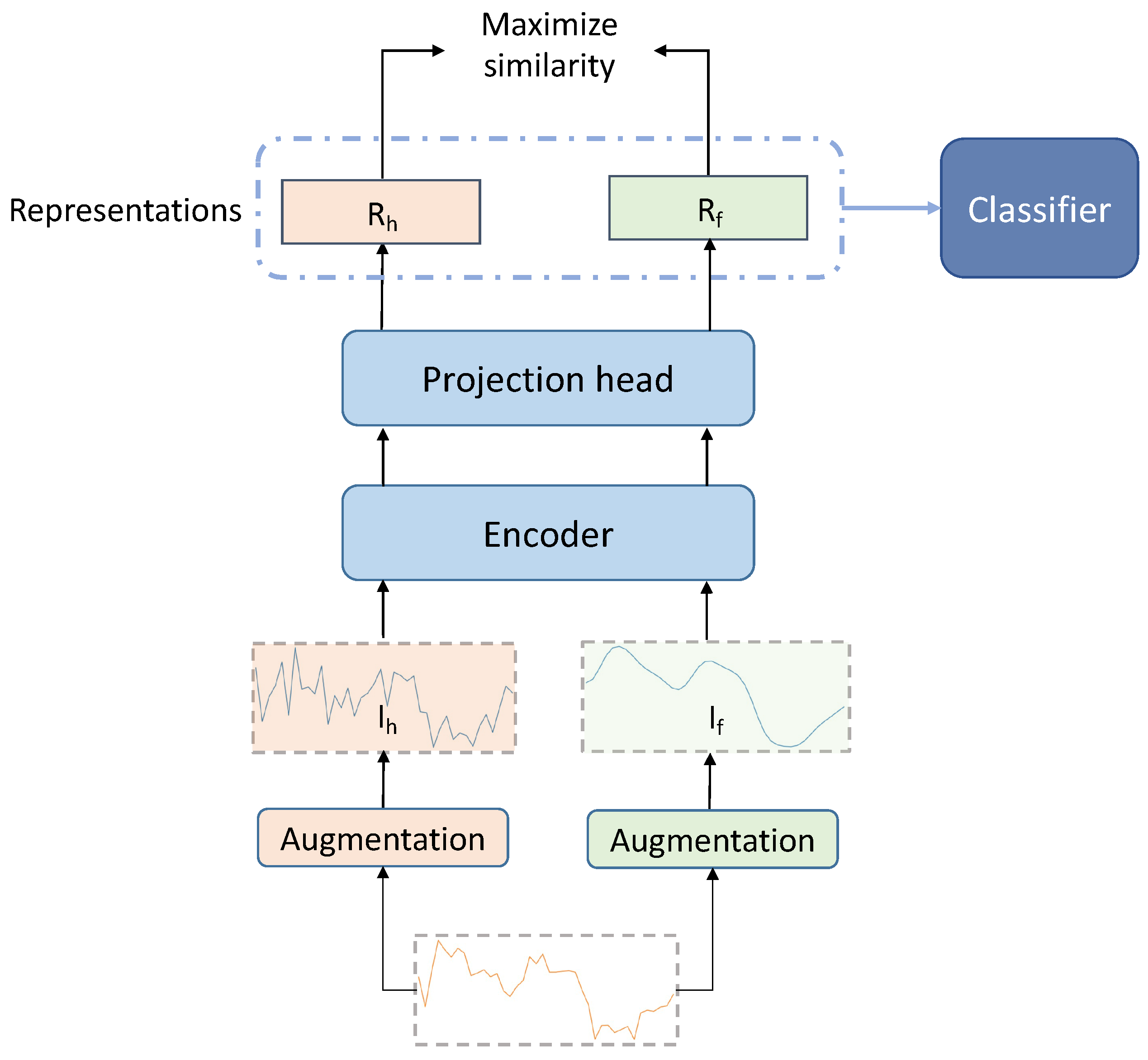
Figure 1. Illustration of the proposed model architecture.
Stats 07 00025 g001
Figure 2. Illustration of a batch construction.
Stats 07 00025 g002
Figure 3. The TCN encoder architecture.
Stats 07 00025 g003
Figure 4. The projection head architecture.
Stats 07 00025 g004
Figure 5. Visualization of the used data augmentation methods. In each panel, original time series data is in orange and augmented data is in blue.
Stats 07 00025 g005
Figure 6. An example of the knots and the cubic spline using in magnitude-warping.
Stats 07 00025 g006
Figure 7. An example of the horizontally scaled data points using in time-warping.
Stats 07 00025 g007
Figure 8. The experiment results on the sensitivity of window size, batch size and code size.
Stats 07 00025 g008
Figure 9. Effect of batch size across different window sizes.
Stats 07 00025 g009
Figure 10. Effect of code size across different window sizes.
Stats 07 00025 g010
Figure 11. CL-TCN pre-training loss and similarity trajectory.
Stats 07 00025 g011
Figure 12. CL-LSTM pre-training loss and similarity trajectory.
Stats 07 00025 g012
Figure 13. LPPLS confidence indicator result on test set.
Stats 07 00025 g013
Figure 14. CL indicator result on test set.
Stats 07 00025 g014
Table 1. Literature summary of contrastive learning based on time series data.
PaperFrameworkDataTask
Mohsenvand et al., 2020 [23]SimCLRnon-financialClassification
Deldari et al., 2021 [28]CPCnon-financialChange point detection
Hou et al., 2021 [29]CPCCSI-300, CSI-800, NASDAQ100Stock Trend Prediction
Wang et al., 2021 [30]CPCACL18, KDD17Stock Trend Prediction
Eldele et al., 2022 [25] non-financialClassification
Poppelbaum et al., 2022 [27]SimCLRnon-finanicalClassification
Feng et al., 2022 [31]SimCLRCSI-500Stock Trend Prediction
Yue et al., 2022 [26] non-financialClassification
Zhan et al., 2022 [32]SimCLRACL18, KDD17Stock Trend Prediction
Zhang et al., 2022 [33] non-financialClassification
Table 2. Summary of all selected peaks.
Peak DayPeak PriceEnd DayEnd PriceDropDuration
2014-11-12423.62015-01-14178.158.0%63
2015-03-11296.42015-04-14219.226.1%34
2015-07-12310.92015-08-24210.532.3%43
2015-12-15465.32016-01-15364.321.7%31
2016-06-16766.32016-08-02547.528.6%47
2017-01-041154.72017-01-11777.832.6%7
2017-03-031275.02017-03-24937.526.5%21
2017-06-112958.12017-07-161929.834.8%35
2017-09-014892.02017-09-143154.935.5%13
2017-12-1619,497.42018-02-056955.364.3%51
2018-03-0511,573.32018-04-066636.342.7%32
2018-05-059858.22018-06-285903.440.1%54
2018-07-248424.32018-08-106184.726.6%17
2019-06-2613,016.22019-07-169477.627.2%20
2019-10-279551.72019-12-176640.530.5%51
2020-02-1210,326.12020-03-124970.851.9%29
2021-04-1363,503.52021-04-2549,004.322.8%12
2021-09-0652,633.52021-09-2140,693.722.7%15
2021-11-0867,566.82022-01-2235,030.348.2%75
2022-03-2947,465.72022-06-1819,017.659.9%81
2022-08-1324,424.12022-09-0618,837.722.9%24
Table 3. Details of training set and test set.
TrainingTest
period2014-10-30∼2021-02-182021-02-19∼2022-09-17
# windows2304576
# label = 122470
Table 4. Time series features used in ML models including those based on sample ACFs, PACFs, and other time series features.
Category#FeaturesFeatures
General5median, min, max, skewness, kurtosis
ACF6acf1, acf10, dacf1, dacf10, d2acf1, d2acf10
PACF3pacf5, dpacf5, d2pacf5
STL6trend, spike, linearity, curvature, stl1, stl10
Other7nonlinearity, entropy, lumpiness, stability, max_level_shift, max_var_shift, max_kl_shift
Table 5. Configuration parameters for grid-search of ML classifiers.
ModelParametersValues
RFn_estimators100, 150, 200, 250
max_depth5, 6, 7, 8
SVMC0.1, 1, 10, 100
gamma0.001, 0.01, 0.1, 1
kernelsigmiod, rbf, poly
GBMlearning_rate0.01, 0.03, 0.1, 0.3
n_estimators100, 150, 200, 250
subsample0.6, 0.8, 1
max_depth5, 6, 7, 8
XGBlearning_rate0.01, 0.03, 0.1, 0.3
n_estimators100, 150, 200, 250
subsample0.6, 0.8, 1
max_depth5, 6, 7, 8
Table 6. Search space and filter conditions for the qualification of valid LPPLS fits used in this study.
ItemNotationSearch SpaceFiltering Condition
3 nonlinear parametersm [ 0 , 2 ] [ 0.01 , 0.99 ]
ω [ 1 , 50 ] [ 2 , 25 ]
t c [ t 2 0.2 d t , [ t 2 ,
t 2 + 0.2 d t ] t 2 + 0.1 d t ]
Number of oscillations ω 2 ln | t c t 1 t 2 t 1 | [ 2.5 , + ]
Damping m | B | ω | C | [ 1 , + )
Relative error p t p t ^ p t ^ [ 0 , 0.2 ]
Table 7. Performance on drawdowns prediction of CL with one head.
AugmentationF2GMBAFM
None 0.29 ± 0.15 0.51 ± 0.14 0.57 ± 0.11 0.25 ± 0.12
Jittering 0.49 ± 0.00 0.62 ± 0.09 0.67 ± 0.03 0.40 ± 0.01
Scaling 0.34 ± 0.26 0.48 ± 0.25 0.57 ± 0.17 0.28 ± 0.21
Magnitude-warping 0.44 ± 0.03 0.56 ± 0.16 0.63 ± 0.06 0.37 ± 0.01
Time-warping 0.54 ± 0.06 0.71 ± 0.04 0.72 ± 0.04 0.44 ± 0.04
Crop-and-resize 0.23 ± 0.19 0.43 ± 0.22 0.56 ± 0.09 0.21 ± 0.16
Smoothing 0.16 ± 0.24 0.26 ± 0.33 0.45 ± 0.19 0.13 ± 0.19
Table 8. Performance on drawdowns prediction of CL with two head.
AugmentationF2GMBAFM
None, None 0.29 ± 0.15 0.51 ± 0.14 0.57 ± 0.11 0.25 ± 0.12
Jittering, Time-warping 0.37 ± 0.14 0.57 ± 0.10 0.60 ± 0.09 0.31 ± 0.11
Jittering, Magnitude-warping 0.39 ± 0.11 0.60 ± 0.10 0.63 ± 0.07 0.33 ± 0.09
Time-warping, Magnitude-warping 0.36 ± 0.13 0.46 ± 0.21 0.51 ± 0.17 0.30 ± 0.12
Table 9. Performance on drawdowns prediction of CL with augmentation combinations on one head.
AugmentationF2GMBAFM
None, None 0.29 ± 0.15 0.51 ± 0.14 0.57 ± 0.11 0.25 ± 0.12
Jittering, Time-warping 0.45 ± 0.17 0.63 ± 0.15 0.64 ± 0.15 0.37 ± 0.14
Jittering, Magnitude-warping 0.28 ± 0.19 0.44 ± 0.18 0.57 ± 0.07 0.27 ± 0.18
Time-warping, Magnitude-warping 0.55 ± 0.08 0.73 ± 0.05 0.74 ± 0.06 0.45 ± 0.05
Table 10. Comparison of models performance on drawdowns prediction for daily data.
F2GMBAFM
RF 0.30 ± 0.02 0.53 ± 0.01 0.57 ± 0.01 0.26 ± 0.01
SVM 0.09 ± 0.10 0.25 ± 0.15 0.49 ± 0.05 0.09 ± 0.08
GBM 0.36 ± 0.04 0.57 ± 0.03 0.58 ± 0.02 0.29 ± 0.03
XGB0.46 ± 0.0040.66 ± 0.0030.66 ± 0.0030.37 ± 0.003
LSTM 0.12 ± 0.08 0.31 ± 0.12 0.51 ± 0.01 0.13 ± 0.06
TCN0.50 ± 0.070.68 ± 0.04 0.69 ± 0.050.40 ± 0.06
CL-LSTM 0.36 ± 0.04 0.49 ± 0.05 0.53 ± 0.03 0.29 ± 0.03
CL-TCN0.54 ± 0.060.71 ± 0.040.72 ± 0.040.44 ± 0.04
Table 11. Performance on drawdowns prediction of ensemble models, compared with CL-TCN.
Simple AverageWeighted AverageHard VoteLogisticCL-TCN
F20.5340.4950.5160.3110.535
GM0.7100.6870.7000.5380.711
BA0.7150.6870.7000.5750.722
FM0.4300.4000.4160.2650.436
Table 12. Performance on drawdowns prediction of LPPLS indicator and CL-TCN indicator.
LPPLS-IndicatorCL-Indicator
F20.0750.423
GM0.2540.634
BA0.4870.642
FM0.0810.349
Disclaimer/Publisher’s Note: The statements, opinions and data contained in all publications are solely those of the individual author(s) and contributor(s) and not of MDPI and/or the editor(s). MDPI and/or the editor(s) disclaim responsibility for any injury to people or property resulting from any ideas, methods, instructions or products referred to in the content.