New Goodness-of-Fit Tests for the Kumaraswamy Distribution

Abstract

The two-parameter distribution known as the Kumaraswamy distribution is a very flexible alternative to the beta distribution with the same (0,1) support. Originally proposed in the field of hydrology, it has subsequently received a good deal of positive attention in both the theoretical and applied statistics literatures. Interestingly, the problem of testing formally for the appropriateness of the Kumaraswamy distribution appears to have received little or no attention to date. To fill this gap, in this paper, we apply a “biased transformation” methodology to several standard goodness-of-fit tests based on the empirical distribution function. A simulation study reveals that these (modified) tests perform well in the context of the Kumaraswamy distribution, in terms of both their low size distortion and respectable power. In particular, the “biased transformation” Anderson–Darling test dominates the other tests that are considered.

1. Introduction

The two-parameter distribution introduced by Kumaraswamy [1] is a very flexible alternative to the beta distribution with the same (0,1) support. Originally proposed for the analysis of hydrological data, it has subsequently received a good deal of attention in both the theoretical and applied statistics literature. For example, Sundar and Subbiah [2], Seifi et al. [3], Ponnambalam et al. [4], Ganji et al. [5], and Courard-Hauri [6] provide applications in various fields, and theoretical extensions are implemented by Cordeiro and Castro [7], Bayer et al. [8], and Cordeiro et al. [9], among others.

The distribution function for a random variable, X, that follows the Kumaraswamy distribution is as follows:

$$F\left(x\right)=1-{\left(1-x^a\right)}^b\hspace{1em}\hspace{1em}a, b>0;\hspace{1em}0<x<1,$$

(1)

which can be inverted to give the quantile function as follows:

$$Q\left(y\right)\equiv F^{-1}\left(y\right)={\left[1-{(1-y)}^{1/b}\right]}^{1/a}\hspace{1em};\hspace{1em}\hspace{1em}\hspace{1em}0<y<1$$

(2)

The corresponding density function is as follows:

$$f\left(x\right)=ab{x}^{a-1}{(1-x^a)}^{b-1}$$

(3)

where ‘a’ and ‘b’ are both shape parameters. Some examples of the forms that this density can take are illustrated in Figure 1. In particular, similarly to the beta density, $f\left(x\right)$ is unimodal if $a>1$ and $b>1$; uniantimodal if $a<1$ and $b<1$; increasing (decreasing) in x if $a>1$ and $b\le 1$ ($a\le 1$ and $b>1$); and constant if $a=b=1$. Nadarajah [10] notes that the Kumaraswamy distribution is in fact a special case of the generalized beta distribution proposed by McDonald [11].

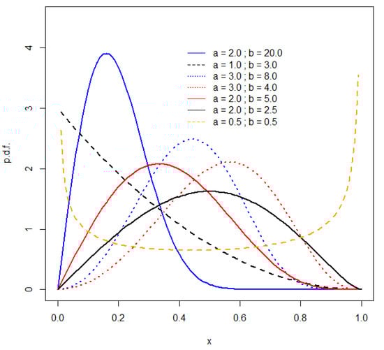
Figure 1. Kumaraswamy densities.

Jones [12] notes that the r’th central moment of the Kumaraswamy distribution exists if $r>-a$ and is given by the following:

$$E\left(X^r\right)=bB\left(1+\frac{r}{a},b\right)$$

(4)

where B (., .) is the complete beta function; and from (2), the median of the distribution is as follows:

$$m_d{=\left[1-{0.5}^{\raisebox{1ex}{$1$}\!\left/ \!\raisebox{-1ex}{$b$}\right.}\right]}^{\raisebox{1ex}{$1$}\!\left/ \!\raisebox{-1ex}{$a$}\right.}$$

(5)

See Jones [12], Garg [13], and Mitnik [14] for a detailed discussion of the additional properties of the Kumaraswamy distribution.

These properties, compared with those of the beta distribution, are considered by many to give the Kumaraswamy distribution a competitive edge. For example, compared with the formula for the cumulative distribution function of the beta distribution, the invertible closed-form expression in (1) is seen by some as being advantageous in the context of computer-intensive simulation analyses and modelling based on quantiles. The latter consideration is of particular interest in the context of regression analyses. Beta regression, based on the closed-form mean of the distribution, is well established (e.g., Ferrari and Cribari-Neto [15]), but robust regression based on the median is impractical. In contrast, the median of the Kumaraswamy distribution has a simple form, given in (5), and so robust regression based on this distribution is straightforward. See Mitnik and Baek [16] and Hamedi-Shahraki et al. [17], for example.

Interestingly, the problem of testing formally for the appropriateness of the Kumaraswamy distribution appears to have received little or no attention in the literature. Goodness-of-fit tests based on the empirical distribution function (EDF) are obvious candidates, but their properties are unexplored for this distribution. Raschke [18] observed that such tests were unavailable for the beta distribution, and he proposed a “biased transformation” that he then applied to the test of Anderson and Darling [19,20] to fill this gap. He also used this approach to construct an EDF test for the gamma distribution. Subsequently, Raschke [21] provided extensive simulation results that favoured the use of the “bias-transformed” Anderson–Darling test over various other tests based on the EDF, such as those of Kuiper [22] and Watson [23], the Cramér–von Mises test (Cramér [24]; von Mises [25]), and the Kolmogorov–Smirnov test (Kolmogorov [26]; Smirnov [27]).

In this paper, we apply Raschke’s methodology to the problem of constructing EDF goodness-of-fit tests for the Kumaraswamy distribution, and we compare the performances of several such standard tests in terms of both size and power. We find that Raschke’s method performs well in this context, with the Kolmogorov–Smirnov and Cramér–von Mises tests exhibiting the least size distortion, and the Anderson–Darling test being a clear choice in terms of power against a wide range of alternatives.

In the next section, we introduce the “biased transformation” testing strategy suggested by Raschke and describe the five well-known EDF tests that we consider in this paper. Section 3 provides the results of a simulation experiment that evaluates the sizes and powers of the tests, and an empirical application is included in Section 4. Some concluding remarks are presented in Section 5.

2. Raschke’s “Biased Transformation” Testing

In very simple terms, the procedure proposed by Raschke involves the use of a transformation that converts the problem of testing the null hypothesis that the data follow the Kumaraswamy distribution into one of testing the null hypothesis of normality. The latter, of course, is readily performed using standard EDF tests. More specifically, the steps involved are as follows (Raschke [21]):

(i)

Assuming that the data, X, follow the Kumaraswamy distribution, estimate the shape parameters, a and b, using maximum likelihood (ML) estimation. See Lemonte [28] and Jones [12] for details of the ML estimator for this distribution;

(ii)

Using these parameter estimates, generate a sample of Y, where $Y={\mathsf{\Phi }}^{-1}(F(X))$, $\mathsf{\Phi }$ is the distribution function for the standard normal distribution, and $F(.)$ is given in (1);

(iii)

Obtain the ML estimates of the parameters of the normal distribution for Y;

(iv)

Apply an EDF test for normality to the Y data;

(v)

For a chosen significance level, α, reject $H_0:$ “X is Kumaraswamy” if $H_0^{\prime }:$ “Y is Normal” is rejected.

We consider five standard EDF tests for normality at step (iv), with the n values of the Y data in ascending order. See Stephens [29] for more details. The first two of these tests are based on the two quantities $D^{+}={\mathrm{m}\mathrm{a}\mathrm{x}}_{\left(i\right)}[i/n-F(Y_i\left)\right]$, $D^{-}={\mathrm{m}\mathrm{a}\mathrm{x}}_{\left(i\right)}[F\left(Y_i\right)-(i-1)/n]$ and $D=\mathrm{m}\mathrm{a}\mathrm{x}[D^{+},D^{-}]$. The Kolmogorov–Smirnov test statistic is $D*=D(\sqrt{n}-0.01+0.85/\sqrt{n})$, and Kuiper’s test statistic is $V*=V(\sqrt{n}+0.05+0.82/\sqrt{n})$, where $V=(D^{+}+D^{-})$. In each case, $H_0^{\prime }$ is rejected if the test statistic exceeds the appropriate critical value.

Further, defining $W^2=\sum _{i=1}^n{[F\left(Y_i\right)-(2i-1)/(2n\left)\right]}^2$, the Cramér–von Mises test statistic is given by $W^{2\ast }=W^2(1.0+0.5/n))$. Similarly, if $U^2=W^2-n\{\sum _{i=1}^n{[F\left(Y_i]/n\right)-0.5\}}^2$, the Watson test statistic is defined as $U^{2\ast }=U^2(1.0+0.5/n)$. Finally, the Anderson–Darling test statistic is defined as $A^{2\ast }=A^2(1.0-0.75/n/+2.25/n^2)$, where $A^2=-n-\sum _{i=1}^n\left\{\left(2i-1\right)\left(ln\left[F\left(Y_i\right)\right]+\ln \left[1-F\left(Y_{n+1-i}\right)\right]\right)\right\}/n$. Again, for these last three tests, the null hypothesis is rejected if the test statistic exceeds the appropriate critical value. In the next section, we consider nominal significance levels of α = 5% and α =10%. The critical values for the five tests are from Table 4.7 of Stephens [29]. They are reported in the last row of Table 1 in the next section, to the degree of accuracy provided by Stephens.

Table 1. Simulated sizes of the EDF tests for various shape parameter values *.

n	K-S	Kuiper	C-M	Watson	A-D	K-S	Kuiper	C-M	Watson	A-D
a = 3, b = 4
			α = 5%					α = 10%
10	0.0585	0.0597	0.0561	0.0550	0.0638	0.1193	0.1210	0.1133	0.1189	0.1277
25	0.0492	0.0464	0.0482	0.0486	0.0487	0.1053	0.0978	0.0990	0.1015	0.1037
50	0.0505	0.0475	0.0459	0.0451	0.0472	0.1007	0.0981	0.0941	0.0977	0.0982
100	0.0497	0.0467	0.0488	0.0480	0.0486	0.1002	0.0925	0.0932	0.0967	0.0949
a = 3, b = 8
			α = 5%					α = 10%
10	0.0577	0.0593	0.0559	0.0551	0.0628	0.1174	0.1209	0.1130	0.1178	0.1255
25	0.0479	0.0460	0.0474	0.0481	0.0485	0.1040	0.0972	0.0978	0.1013	0.1033
50	0.0498	0.0470	0.0447	0.0434	0.0463	0.1002	0.0969	0.0924	0.0976	0.0972
100	0.0494	0.0462	0.0481	0.0475	0.0475	0.0986	0.0926	0.0922	0.0956	0.0927
a = 2, b = 2.5
			α = 5%					α = 10%
10	0.0598	0.0590	0.0570	0.0560	0.0642	0.1184	0.1214	0.1133	0.1192	0.1267
25	0.0500	0.0470	0.0486	0.0486	0.0496	0.1048	0.0981	0.0991	0.1019	0.1034
50	0.0515	0.0479	0.0460	0.0460	0.0479	0.1021	0.0988	0.0951	0.0986	0.0985
100	0.0489	0.0468	0.0496	0.0494	0.0492	0.1010	0.0929	0.0946	0.0974	0.0957
a = 2.0, b = 5.0
			α = 5%					α = 10%
10	0.0586	0.0597	0.0557	0.0550	0.0630	0.1184	0.1208	0.1130	0.1184	0.1269
25	0.0491	0.0463	0.0478	0.0486	0.0489	0.1055	0.0977	0.0983	0.1015	0.1032
50	0.0503	0.0472	0.0457	0.0445	0.0468	0.1003	0.0973	0.0931	0.0976	0.0976
100	0.0496	0.0464	0.0488	0.0474	0.0485	0.1000	0.0923	0.0930	0.0959	0.0941
a = 2.0, b = 20.0
			α = 5%					α = 10%
10	0.0576	0.0593	0.0550	0.0550	0.0620	0.1170	0.1205	0.1106	0.1172	0.1248
25	0.0473	0.0455	0.0474	0.0481	0.0476	0.1034	0.0969	0.0978	0.1018	0.1022
50	0.0492	0.0464	0.0442	0.0430	0.0456	0.0999	0.0963	0.0911	0.0974	0.0964
100	0.0485	0.0463	0.0469	0.0466	0.0459	0.0978	0.0923	0.0913	0.0943	0.0923
a = 1.0, b = 3.0
			α = 5%					α = 10%
10	0.0589	0.0592	0.0560	0.0553	0.0642	0.1189	0.1209	0.1131	0.1192	0.1273
25	0.0497	0.0464	0.0486	0.0486	0.0493	0.1051	0.0980	0.0993	0.1021	0.1037
50	0.0512	0.0477	0.0460	0.0455	0.0474	0.1014	0.0986	0.0948	0.0981	0.0985
100	0.0495	0.0470	0.0493	0.0487	0.0487	0.1002	0.0926	0.0940	0.0968	0.0955
a = 0.5, b = 0.5
			α = 5%					α = 10%
10	0.0625	0.0603	0.0574	0.0582	0.0679	0.1260	0.1199	0.1179	0.1203	0.1346
25	0.0592	0.0527	0.0619	0.0590	0.0643	0.1154	0.1071	0.1158	0.1168	0.1235
50	0.0650	0.0571	0.0689	0.0624	0.0742	0.1267	0.1165	0.1285	0.1238	0.1366
100	0.0864	0.0730	0.0940	0.0819	0.1017	0.1563	0.1356	0.1605	0.1509	0.1706
Crit.	0.895	1.489	0.126	0.117	0.752	0.819	1.386	0.104	0.096	0.631

* Crit. = Upper-tail critical values when the normal distribution’s parameters are both estimated. Source: Stephen [29], Table 4.7. (Stephens reports these values to only 3 decimal places). α = nominal significance level at which the tests are applied. K-S = Kolmogorov and Smirnov; C-M = Cramér and von Mises; and A-D = Anderson and Darling.

3. A Simulation Study

Using Raschke’s “biased transformation”, each of the five EDF tests for the Kumaraswamy null hypothesis has been evaluated in a simulation experiment, using R (R Core Team [30]). In all parts of the Monte Carlo study, 10,000 Monte Carlo replications were used. The ‘univariateML’ package (Moss and Nagler [31]) was used for obtaining the ML estimates of the Kumaraswamy distribution in step (i), and the ‘GoFKernel’ package (Pavia [32]) was used to invert the distribution in step (ii) in the last section. Random numbers for the truncated log-normal and triangular distribution were generated using the ‘EnvStats’ package (Millard and Kowarik [33]), while those for the Kumaraswamy distribution itself were generated using the ‘VGAM’ package (Yee [34]). The ‘trapezoid’ package (Hetzel [35]) and the ‘truncnorm’ package (Mersmann et al. [36]) were used to generate random variates from the trapezoidal and truncated normal distributions, respectively, and the R base ‘stats’ package was used for the beta variates. Finally, random variates from the truncated gamma distribution were generated using the ‘cascsim’ package (Bear et al. [37]), and those for the truncated Weibull distribution were obtained using the ‘ReIns’ package (Reynkens [38]). The R code that was used for both parts of the simulation experiment is available for download from https://github.com/DaveGiles1949/r-code/blob/master/Kumaraswmay%20Paper%20EDF%20Power%20Study.R (accessed on 5 March 2024).

In the first part of the experiment, we investigate the true “size” of each of the five EDF tests for various sample sizes (n) and a selection of values of the parameters (a and b) of the null distribution. As noted above, the tests are applied using nominal significance levels of both 5% and 10%, and we are concerned here with the extent of any “size distortion” that may arise.

The results obtained with seven representative (a,b) pairs and sample sizes ranging from n = 10 to n = 100 are shown in Table 1. The corresponding Kumaraswamy densities appear in Figure 1. The simulated sizes of all of the tests are very close to the nominal significance levels in all cases. This result is very encouraging and provides initial support for adopting the “biased transformation” EDF testing strategy for the Kumaraswamy distribution.

Of the five tests considered, the Kolmogorov–Smirnov test performs best, in terms of the least absolute difference between the nominal and simulated sizes in 16 of the 36 cases at the 5% nominal level and 10 of the 36 cases at the 10% nominal level, as shown in Table 1. In the latter case, it is outperformed by the Cramér–von Mises test, which dominates for 14 of the 36 cases that are considered. Further, there is a general tendency for the simulated sizes of all of the tests to exceed the nominal significance levels when $n\le 25$, while the converse is true (in general) when $n\ge 50$. An exception is when both of the distributions’ parameters equal 0.5, in which case the density is uniantimodal. These size distortions are generally small, but their direction has implications for the results relating to the powers of the tests.

The second part of the Monte Carlo experiment investigates the powers of the five tests against a range of alternative hypotheses. The latter all involve distributions on the (0,1) interval, with some distributions truncated accordingly. It should be noted that the simulated powers that are reported are “raw powers” and are not “size-adjusted”. That is, the various critical values that are used are those reported at the end of Table 1. In practical applications, this is how a researcher would proceed.

The results of this part of the study are reported in Table 2. The sample sizes range from n = 10 to n = 1000. A wide range of parameter values was considered for each of the alternative distributions, and a representative selection of the results that were obtained are reported here. For the truncated log-normal distribution, “meanlog” is the mean of the distribution of the non-truncated random variable on the log scale, and “sdlog” is the standard deviation of the distribution of the non-truncated random variable on the log scale. For the trapezoidal distribution, m₁ and m₂ are the first and second modes, n₁ is the growth parameter, and n₃ is the decay parameter.

Table 2. Simulated powers of the EDF tests against various alternative hypotheses.

n	K-S	Kuiper	C-M	Watson	A-D	K-S	Kuiper	C-M	Watson	A-D
Triangular (mode = 1/4)
			α = 5%					α = 10%
10	0.0784	0.0752	0.0765	0.0754	0.0878	0.1439	0.1409	0.1426	0.1463	0.1604
25	0.0978	0.0868	0.1097	0.0987	0.1175	0.1766	0.1550	0.1857	0.1785	0.1988
50	0.1422	0.1218	0.1707	0.1498	0.1806	0.2397	0.2061	0.2597	0.2422	0.2742
100	0.2470	0.2121	0.3051	0.2639	0.3160	0.3740	0.3182	0.4157	0.3773	0.4333
250	0.5491	0.4885	0.6490	0.5831	0.6723	0.6762	0.6224	0.7564	0.703	0.7712
500	0.8529	0.8178	0.9246	0.8865	0.9347	0.9196	0.8940	0.9573	0.9351	0.9637
1000	0.9929	0.9909	0.9978	0.9961	0.9986	0.9975	0.9963	0.9992	0.9986	0.9994
Triangular (mode = 7/8)
			α = 5%					α = 10%
10	0.0676	0.0711	0.0660	0.0644	0.0755	0.1314	0.1330	0.1283	0.1353	0.1446
25	0.0736	0.0680	0.0822	0.0768	0.0866	0.1422	0.1294	0.1455	0.1462	0.1538
50	0.0969	0.0884	0.1144	0.1052	0.1233	0.1797	0.1626	0.1966	0.1854	0.2124
100	0.1575	0.1336	0.1928	0.1659	0.2191	0.2561	0.2294	0.2964	0.2703	0.3264
250	0.3588	0.3192	0.4530	0.3883	0.5122	0.5053	0.4532	0.5853	0.5231	0.6366
500	0.6568	0.6198	0.7771	0.6994	0.8386	0.7845	0.7446	0.8622	0.8127	0.9001
1000	0.9364	0.9310	0.9789	0.9603	0.9890	0.9730	0.9671	0.9904	0.9815	0.9954
Truncated Log-Normal (meanlog = 0, sdlog = 1)
			α = 5%					α = 10%
10	0.0774	0.0758	0.0762	0.0738	0.0883	0.1458	0.1409	0.1420	0.1452	0.1614
25	0.1011	0.0862	0.1147	0.1003	0.1260	0.1836	0.1560	0.1918	0.1796	0.2139
50	0.1536	0.1212	0.1836	0.1548	0.2073	0.2533	0.2037	0.2842	0.2528	0.3148
100	0.2778	0.2193	0.3431	0.2785	0.3907	0.4153	0.3310	0.4672	0.4035	0.5182
250	0.6143	0.5376	0.7436	0.6318	0.8054	0.7399	0.6646	0.8319	0.7519	0.8795
500	0.9105	0.8815	0.9713	0.9290	0.9867	0.9600	0.9397	0.9870	0.9657	0.9936
1000	0.9981	0.9975	1.0000	0.9992	1.0000	0.9996	0.9994	1.0000	0.9999	1.0000
Truncated Log-Normal (meanlog= 0.5, sdlog = 0.5)
			α = 5%					α = 10%
10	0.0398	0.0400	0.0375	0.0382	0.0432	0.0786	0.0757	0.0751	0.0765	0.0841
25	0.0653	0.0589	0.0672	0.0635	0.0718	0.1303	0.1167	0.1313	0.1272	0.1382
50	0.0798	0.0671	0.0868	0.0760	0.0956	0.1503	0.1290	0.1539	0.1459	0.1673
100	0.1164	0.0924	0.1349	0.1106	0.1474	0.1997	0.1679	0.2168	0.1946	0.2374
250	0.2427	0.1834	0.2966	0.2365	0.3371	0.3668	0.2937	0.4120	0.354	0.4568
500	0.4474	0.3538	0.5422	0.4401	0.6156	0.5861	0.4880	0.6661	0.5742	0.7337
1000	0.7557	0.6784	0.8670	0.7678	0.9163	0.8594	0.7980	0.9255	0.8623	0.9582
Truncated Normal (mean = 0.5, sd = 0.1)
			α = 5%					α = 10%
10	0.0704	0.0648	0.0686	0.0629	0.0799	0.1348	0.1253	0.1260	0.1287	0.1476
25	0.0839	0.0770	0.0952	0.0856	0.1076	0.1540	0.1368	0.1644	0.1517	0.1798
50	0.1188	0.0986	0.1395	0.1166	0.1607	0.2031	0.1698	0.2209	0.1991	0.2457
100	0.1928	0.1506	0.2309	0.1868	0.2682	0.3029	0.2497	0.3393	0.2945	0.3834
250	0.4263	0.3493	0.5179	0.4206	0.5840	0.5625	0.4782	0.6409	0.5542	0.6987
500	0.7151	0.6509	0.8345	0.7321	0.8822	0.8227	0.7661	0.8988	0.8336	0.9310
1000	0.9516	0.9408	0.9891	0.9675	0.9957	0.9813	0.9723	0.9954	0.9857	0.9984
Truncated Normal (mean = 0.8, sd = 0.8)
			α = 5%					α = 10%
10	0.0577	0.0586	0.0547	0.0559	0.0647	0.1170	0.1166	0.1137	0.1163	0.1306
25	0.0519	0.0500	0.0529	0.0517	0.0540	0.1040	0.0981	0.1045	0.1080	0.1096
50	0.0544	0.0507	0.0584	0.0559	0.0573	0.1081	0.1003	0.1044	0.1063	0.1088
100	0.0558	0.0544	0.0558	0.0552	0.0574	0.1193	0.1075	0.1115	0.1126	0.1154
250	0.0681	0.0657	0.0720	0.0692	0.0765	0.1293	0.1244	0.1284	0.1241	0.1349
500	0.0873	0.0867	0.0999	0.0904	0.1099	0.1648	0.1578	0.1696	0.1628	0.1790
1000	0.1404	0.1300	0.1566	0.1410	0.1717	0.2318	0.2196	0.2476	0.2374	0.2695
Trapezoidal (m1 = 1/8, m2 = 3/8; n1 = n3 = 2)
			α = 5%			α = 10%
10	0.0636	0.0652	0.0606	0.0605	0.0691	0.1250	0.1249	0.1193	0.1254	0.1372
25	0.0632	0.0570	0.0651	0.0620	0.0730	0.1282	0.1169	0.1293	0.1261	0.1400
50	0.0771	0.0652	0.0830	0.0703	0.0968	0.1473	0.1275	0.1537	0.1417	0.1704
100	0.1124	0.0877	0.1292	0.1054	0.1531	0.1934	0.1616	0.2146	0.1889	0.2477
250	0.2306	0.1772	0.2885	0.2196	0.3537	0.3521	0.2873	0.4103	0.3433	0.4821
500	0.4214	0.3613	0.5405	0.4248	0.6512	0.5705	0.4937	0.6686	0.5650	0.7640
1000	0.7258	0.7011	0.8737	0.7625	0.9371	0.8409	0.8148	0.9322	0.8639	0.9694
Trapezoidal (m1 = 5/8, m2 = 7/8; n1 = n3 = 2)
			α = 5%			α = 10%
10	0.0587	0.0618	0.0570	0.0575	0.0678	0.1221	0.1241	0.1172	0.1232	0.1331
25	0.0553	0.0518	0.0570	0.0572	0.0603	0.1136	0.1040	0.1121	0.1151	0.1176
50	0.0628	0.0577	0.0622	0.0580	0.0681	0.1185	0.1102	0.1231	0.1201	0.1309
100	0.0726	0.0637	0.0822	0.0740	0.0936	0.1439	0.1222	0.1477	0.1390	0.1635
250	0.1270	0.1021	0.1473	0.1203	0.1781	0.2181	0.1827	0.2343	0.2051	0.2822
500	0.2183	0.1782	0.2735	0.2157	0.3452	0.3429	0.2856	0.3934	0.3329	0.4788
1000	0.3973	0.3560	0.5320	0.4180	0.6536	0.5543	0.5058	0.6674	0.5676	0.7692
Trapezoidal (m1 = 1/4, m2 = 3/4; n1 =n3 = 3)
			α = 5%			α = 10%
10	0.0626	0.0732	0.0637	0.0687	0.0719	0.1271	0.1389	0.1291	0.1395	0.1439
25	0.0711	0.0862	0.0781	0.0858	0.0809	0.1402	0.1560	0.1517	0.1663	0.1576
50	0.0973	0.1285	0.1224	0.1313	0.1274	0.1860	0.2172	0.2143	0.2302	0.2213
100	0.1543	0.2168	0.2118	0.2317	0.2272	0.2707	0.3330	0.3306	0.3574	0.3496
250	0.3816	0.5086	0.5225	0.5503	0.5607	0.5477	0.6386	0.6588	0.6863	0.6912
500	0.7178	0.8402	0.8635	0.8791	0.8885	0.8447	0.9095	0.9238	0.9322	0.9389
1000	0.9719	0.9914	0.9938	0.9953	0.9969	0.9905	0.9971	0.9983	0.9989	0.9991
Truncated Gamma (2,3)
			α = 5%					α = 10%
10	0.2211	0.2728	0.2364	0.2498	0.3155	0.3266	0.3958	0.3626	0.3759	0.4511
25	0.5018	0.6293	0.5807	0.5813	0.7294	0.6489	0.7385	0.7025	0.7058	0.8269
50	0.8745	0.9442	0.9062	0.9023	0.9748	0.9391	0.9708	0.9516	0.9507	0.9890
100	0.9985	0.9998	0.9989	0.9983	1.0000	0.9997	0.9999	0.9996	0.9996	1.0000
250	1.0000	1.0000	1.0000	1.0000	1.0000	1.0000	1.0000	1.0000	1.0000	1.0000
Truncated Gamma (2,6)
			α = 5%					α = 10%
10	0.1423	0.1321	0.1550	0.1423	0.1834	0.2234	0.2082	0.2346	0.2222	0.2713
25	0.2556	0.2388	0.3222	0.2818	0.3717	0.3662	0.3426	0.4142	0.3788	0.4710
50	0.4407	0.4211	0.5428	0.4775	0.6116	0.5646	0.5251	0.6368	0.5872	0.7005
100	0.7104	0.6954	0.8124	0.7516	0.8649	0.8072	0.7799	0.8703	0.8268	0.9083
250	0.9740	0.9743	0.9910	0.9830	0.9958	0.9878	0.9860	0.9956	0.9906	0.9977
500	0.9998	0.9997	1.0000	0.9997	1.0000	1.0000	0.9999	1.0000	0.9999	1.0000
1000	1.0000	1.0000	1.0000	1.0000	1.0000	1.0000	1.0000	1.0000	1.0000	1.0000
Truncated Weibull (shape = 2, scale = 1)
			α = 5%					α = 10%
10	0.0569	0.0553	0.0508	0.0524	0.0540	0.1138	0.112	0.1052	0.1099	0.1086
25	0.0587	0.0537	0.0608	0.0588	0.0630	0.1192	0.1084	0.1156	0.1148	0.1266
50	0.0643	0.0580	0.0696	0.0644	0.0745	0.1243	0.1168	0.1275	0.1243	0.1345
100	0.0852	0.0702	0.0935	0.0807	0.1004	0.1508	0.1306	0.1563	0.1455	0.1701
250	0.1450	0.1108	0.1607	0.1345	0.1739	0.2354	0.1943	0.2535	0.2244	0.2744
500	0.2478	0.1900	0.2874	0.2381	0.3143	0.3634	0.2943	0.3938	0.3456	0.4239
1000	0.4308	0.3457	0.5167	0.4260	0.5630	0.5717	0.4757	0.6333	0.5563	0.6767
Beta (3,3)
			α = 5%					α = 10%
10	0.0545	0.0573	0.0539	0.0528	0.0606	0.1128	0.1115	0.1065	0.1105	0.1215
25	0.0506	0.0484	0.0534	0.0513	0.0542	0.1047	0.0982	0.1036	0.1054	0.1088
50	0.0527	0.0501	0.0565	0.0542	0.0569	0.1114	0.0975	0.1075	0.1073	0.1149
100	0.0577	0.0532	0.0600	0.0586	0.0629	0.1215	0.1112	0.1186	0.116	0.1232
250	0.0790	0.0641	0.0821	0.0706	0.0897	0.1492	0.1266	0.1492	0.1369	0.1571
500	0.1151	0.0863	0.1148	0.0964	0.1302	0.1939	0.1603	0.1947	0.1714	0.2145
1000	0.1847	0.1339	0.2065	0.1586	0.2340	0.2919	0.2257	0.3078	0.2603	0.3401
Beta (20,20)
			α = 5%					α = 10%
10	0.0710	0.0670	0.0689	0.0664	0.0790	0.1344	0.1288	0.1296	0.1325	0.1493
25	0.0892	0.0765	0.0974	0.0858	0.1100	0.1608	0.1397	0.1738	0.1610	0.1941
50	0.1340	0.1048	0.1629	0.1347	0.1808	0.2313	0.1871	0.2501	0.2235	0.281
100	0.2395	0.1784	0.2922	0.2287	0.3373	0.3682	0.2842	0.4157	0.3494	0.4655
250	0.5380	0.4486	0.6598	0.5398	0.7355	0.6814	0.5858	0.7703	0.6677	0.8338
500	0.8580	0.8040	0.9427	0.8691	0.9692	0.9295	0.8896	0.9719	0.9291	0.9875
1000	0.9925	0.9904	0.9995	0.9953	0.9999	0.9981	0.9968	0.9997	0.9987	0.9999
Beta (4,2)
			α = 5%					α = 10%
10	0.0562	0.0588	0.0562	0.0578	0.0630	0.1155	0.1153	0.1102	0.1138	0.1229
25	0.0509	0.0532	0.0507	0.0503	0.0522	0.1003	0.1019	0.1009	0.1046	0.1072
50	0.0542	0.0516	0.0555	0.0544	0.0574	0.1080	0.0982	0.1050	0.1071	0.1100
100	0.0549	0.0540	0.0562	0.0545	0.0559	0.1079	0.1038	0.1074	0.1076	0.1076
250	0.0672	0.0613	0.0641	0.0579	0.0649	0.1237	0.1134	0.1186	0.1156	0.1232
500	0.0740	0.0647	0.0761	0.0674	0.0795	0.1414	0.1245	0.1346	0.1283	0.1433
1000	0.1048	0.0787	0.1085	0.0905	0.1167	0.1866	0.1489	0.1808	0.1635	0.1956
Beta (2,4)
			α = 5%					α = 10%
10	0.0567	0.0584	0.0533	0.0557	0.0601	0.1118	0.1127	0.1075	0.1131	0.1194
25	0.0521	0.0544	0.0553	0.0539	0.0575	0.1053	0.1032	0.1066	0.1069	0.1120
50	0.0571	0.0539	0.0579	0.0534	0.0587	0.1108	0.1036	0.1121	0.1117	0.1180
100	0.0599	0.0563	0.0631	0.0599	0.0674	0.1168	0.1057	0.1164	0.1116	0.1238
250	0.0799	0.0671	0.0782	0.0689	0.0840	0.1455	0.1262	0.1436	0.1335	0.1569
500	0.1066	0.0835	0.1156	0.0973	0.1254	0.1896	0.1540	0.1897	0.1686	0.2060
1000	0.1720	0.1248	0.1855	0.1498	0.2118	0.2744	0.2068	0.2879	0.2426	0.3124
Beta (3,20)
			α = 5%					α = 10%
10	0.0580	0.0585	0.0562	0.0550	0.0651	0.1180	0.1170	0.1125	0.1147	0.1297
25	0.0662	0.0581	0.0688	0.0640	0.0738	0.1270	0.1182	0.1287	0.1243	0.1413
50	0.0833	0.0678	0.0879	0.0781	0.0953	0.1516	0.1291	0.1574	0.1452	0.1677
100	0.1182	0.0932	0.1374	0.1117	0.1504	0.2104	0.1643	0.2211	0.1936	0.2384
250	0.2426	0.1747	0.2923	0.2226	0.3365	0.3674	0.2825	0.4119	0.3431	0.4621
500	0.4480	0.3450	0.5458	0.4331	0.6145	0.5923	0.4819	0.6718	0.5656	0.7343
1000	0.7586	0.6753	0.8664	0.7577	0.9139	0.8600	0.7928	0.9258	0.8546	0.9548
Beta (0.5,0.5)
			α = 5%					α = 10%
10	0.0547	0.0557	0.0482	0.0491	0.0577	0.1154	0.1121	0.1053	0.1129	0.1224
25	0.0500	0.0506	0.0529	0.0531	0.0542	0.1067	0.0997	0.1073	0.1120	0.1131
50	0.0500	0.0501	0.0532	0.0505	0.0541	0.1048	0.1042	0.1052	0.1102	0.1070
100	0.0538	0.0533	0.0553	0.0542	0.0585	0.1064	0.1056	0.1070	0.1069	0.1086
250	0.0663	0.0615	0.0675	0.0631	0.0702	0.1263	0.1165	0.1235	0.1210	0.1259
500	0.0834	0.0726	0.0853	0.0772	0.0898	0.1551	0.1363	0.1530	0.1457	0.1600
1000	0.1192	0.0993	0.1275	0.1137	0.1363	0.1983	0.1750	0.2071	0.1895	0.2232

One immediate result that emerges is that, with only two exceptions, all of the tests are “unbiased” in all of the settings considered. That is, the power of the test exceeds the nominal significance level. The only exceptions that were encountered are when the alternative distribution is truncated log-normal, with both parameters equal to 0.5 and with a sample size of n = 10. This is a very encouraging result. A test that is “biased” has the unfortunate property that it rejects the null hypothesis less frequently when it is false than when it is true. Moreover, as the various tests are “consistent”, their powers increase as the sample size increases, for any given case.

The results in Table 2 also provide overwhelming support for the Anderson–Darling test in terms of power. Interestingly, this result is totally consistent with the conclusion reached by Raschke [21] for the same “biased transformation” EDF tests in the context of the beta distribution. This may reflect that fact that the latter distribution and the Kumaraswamy distributions have densities that are capable of following very similar shapes, depending on the values of the associated parameters. Moreover, Stephens [29] recommends the Anderson–Darling test over other EDF tests in general.

The Anderson–Darling test has the highest power among all five tests, in all cases, except for very small samples when the alternative distribution is trapezoidal with the parameters m₁ = 1/4 and m₂ = 3/4; when n₁ = n₃ = 3; and for the truncated Weibull alternative with n = 10. Of the other tests under study, the Cramér–von Mises test ranks second in terms of power, followed by Watson’s test and the Kolmogorov–Smirnov test. We find that Kuiper’s test is the least powerful, in general.

As was noted in Section 1, the density for the Kumaraswamy distribution can take shapes very similar to those of the beta density, as the values of the two shape parameters vary in each case. The densities for the alternative beta distributions that are considered in the power analysis are depicted in Figure 2 and may be compared with the Kumaraswamy densities in Figure 1. This similarity suggests that there may be instances in which the proposed EDF tests have relatively low power. If the data are generated by a beta distribution whose characteristics can be mimicked extremely closely by a Kumaraswamy distribution with the same, or similar, shape parameters, the tests may fail to reject the latter distribution. An obvious case in point is when the values of both of these shape parameters are 0.5, and the densities of both distributions are uniantimodal, though not identical. As can be seen in Figure 1, the density for the Kumaraswamy distribution is slightly asymmetric in this case, while its beta distribution counterpart is symmetric. The relatively low power of all of the EDF tests, even for n = 1000, in this case can be seen in the last section of Table 2.

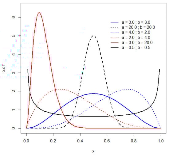
Figure 2. Beta densities.

In view of these observations, we have considered a wide range of different values for the shape parameters associated with the beta distributions that are taken as alternative hypotheses in the power analysis of the EDF tests. A representative selection of the results appears in Table 2. There, we see that although the various tests have modest power when the data are generated by beta (2,4), beta (4,2), and beta (3,3) distributions, they perform extremely well against several other beta alternatives.

Although the degree of size distortion associated with the use of Stephens’ critical values exhibited in Table 1 is generally quite small, a researcher may choose to simulate exact (bias-corrected) critical values for the various EDF tests. It is important to note that such values will depend on the samples size, n, and on the values of the shape parameters, a and b, associated with the Kumaraswamy distribution. In a practical application, the first of these values would be known, and estimates of the shape parameters could be obtained from the sample values in question.

However, the powers of the various tests will also depend on these three values, as well as on the characteristics of the distribution associated with the alternative hypothesis. This complicates the task of illustrating these powers when the critical values are simulated, but Table 3 provides a limited set of results. These results focus on relatively small sample sizes, as the size distortion becomes negligible for large n values. A selection of the alternative hypotheses covered in Table 2 is chosen for further investigation, and the values of the Kumaraswamy shape parameters are chosen to provide the similarity between their shapes and the associated alternatives’ densities. The critical values themselves are obtained as the 90th and 95th percentiles of 10,000 simulated values of each test statistic under the null distribution. There is a different critical value for every entry in Table 3, so they are not reported individually. The powers themselves are then simulated from a further 10,000 replications under the alternative hypothesis, as was the case for the results in Table 2.

Table 3. Simulated powers of the EDF tests with simulated critical values *.

n	K-S	Kuiper	C-M	Watson	A-D	K-S	Kuiper	C-M	Watson	A-D
Triangular (mode = ¼); a = 2, b = 20
			α = 5%					α = 10%
10	0.0649	0.0612	0.0647	0.0638	0.0662	0.1227	0.1124	0.1206	0.1162	0.1251
25	0.0912	0.0829	0.0482	0.1001	0.1021	0.1531	0.1443	0.1715	0.1606	0.1729
50	0.1243	0.1171	0.1527	0.1398	0.1535	0.2146	0.1931	0.2421	0.2224	0.2410
100	0.2078	0.1914	0.2537	0.2269	0.2600	0.3197	0.2906	0.3594	0.3308	0.3644
Truncated-Log-Normal (meanlog = sdlog = 0.5); a= 2, b = 20
			α = 5%					α = 10%
10	0.0507	0.0508	0.0502	0.0496	0.0511	0.1005	0.1015	0.1010	0.0098	0.1001
25	0.0691	0.0617	0.0729	0.0655	0.0757	0.1204	0.1177	0.1334	0.1281	0.1328
50	0.0817	0.0974	0.0970	0.0877	0.1009	0.1494	0.1364	0.1672	0.1531	0.1730
100	0.1253	0.1078	0.1454	0.1274	0.1603	0.2132	0.1856	0.2379	0.2108	0.2600
Trapezoidal (m1 = ¼, m2 = ¾, n1 = n2 = 3); a = 3, b = 8
			α = 5%					α = 10%
10	0.0505	0.0574	0.0527	0.0552	0.0514	0.1073	0.1158	0.1045	0.1114	0.1049
25	0.0697	0.0882	0.0817	0.0874	0.0818	0.1330	0.1562	0.1507	0.1573	0.1530
50	0.0959	0.1328	0.1266	0.1415	0.1311	0.1796	0.2183	0.2218	0.2325	0.2254
100	0.1263	0.2346	0.2299	0.2503	0.2454	0.2820	0.3522	0.3567	0.3770	0.3742
Truncated Gamma (2,3); a = 3, b = 4
			α = 5%					α = 10%
10	0.1924	0.2435	0.2263	0.2353	0.2767	0.3011	0.3435	0.3351	0.3425	0.4010
25	0.5145	0.6463	0.5869	0.5889	0.7374	0.6464	0.7506	0.7104	0.7113	0.8297
50	0.8733	0.9454	0.9143	0.9236	0.9756	0.9392	0.9706	0.9570	0.9528	0.9888
100	0.9978	0.9998	0.9986	0.9979	1.0000	0.9993	0.9999	0.9999	0.9998	1.0000
Beta (20,20); a = 3, b = 8
			α = 5%					α = 10%
10	0.0623	0.0603	0.0651	0.0616	0.0678	0.1201	0.1127	0.1225	0.1201	0.1257
25	0.0942	0.0824	0.1033	0.0907	0.1154	0.1574	0.1457	0.1806	0.1647	0.1921
50	0.1357	0.1126	0.1692	0.1461	0.1934	0.2273	0.1908	0.2704	0.2272	0.2892
100	0.2399	0.1916	0.3063	0.2455	0.3511	0.3659	0.3040	0.4326	0.3610	0.4767
Beta (3,20); a = 2, b = 20
			α = 5%					α = 10%
10	0.0572	0.0544	0.0568	0.0568	0.0565	0.1083	0.1073	0.1093	0.1072	0.1100
25	0.0692	0.0679	0.0755	0.0711	0.0777	0.1242	0.1239	0.1340	0.1254	0.1363
50	0.0822	0.0689	0.0940	0.0846	0.1015	0.1507	0.1312	0.1661	0.1474	0.1738
100	0.1209	0.0993	0.1425	0.1193	0.1595	0.2078	0.1778	0.2329	0.2002	0.2539
Beta (0.5,0.5); a = b = 0.5
			α = 5%					α = 10%
10	0.0442	0.0491	0.0498	0.0501	0.0499	0.0954	0.0966	0.0958	0.0974	0.0938
25	0.0534	0.0552	0.0569	0.0562	0.0546	0.1002	0.1037	0.1026	0.1032	0.1048
50	0.0478	0.0529	0.0524	0.0519	0.0510	0.0965	0.0997	0.1074	0.1092	0.1058
100	0.0549	0.0539	0.0546	0.0532	0.0563	0.1099	0.1100	0.1114	0.1121	0.1141

* a and b are the shape parameters for the Kumaraswamy distribution.

Ranking the various tests in terms of the power results in Table 3 leaves our previous conclusions unchanged. The Anderson–Darling test emerges as the preferred choice. The powers based on the simulated critical values tend to be smaller than their counterparts in Table 2. This is consistent with the earlier observation that the size distortion emerging in that table was positive for small sample sizes.

4. Empirical Applications

To illustrate the effectiveness of the “biased transformation” Anderson–Darling test, we present two applications with actual (economic) data. The R code and associated data files can be downloaded from https://github.com/DaveGiles1949/r-code/blob/master/Kumaraswamy%20Paper%20Applications.R (accessed on 5 March 2024).

4.1. The Hidden Economy

The first application uses data for the size of the so-called “hidden economy” or “underground economy” for 158 countries in each of the years from 1991 to 2017. These data measure the size of the hidden economy (HE) relative to the value of gross domestic product (GDP) in each country and are reported by Medina and Schneider [39]. These ratios range from 0.0543 for Switzerland to 0.5578 for Bolivia, with a mean of 0.2741 and a standard deviation of 0.1120. A random sample of size n = 250 was obtained from this population of 2329 values, using the “sample” command in R with replacement.

When a Kumaraswamy distribution is fitted to the sample data, the estimates of the two shape parameters are 2.8832 and 15.4084. See Figure 3a,b. The value for the “biased transformation” Anderson–Darling statistic is 0.6313, which is less than both the asymptotic and simulated 5% critical values of 0.7520 and 0.7298, respectively. So, at this significance level, we would not reject the hypothesis that the data follow a Kumaraswamy distribution. If a beta distribution is fitted to the data, the estimates of the two shape parameters are 4.3809 and 8.5369. The corresponding Anderson–Darling statistic (using the “biased transformation” and the beta distribution) is 1.3585. This exceeds both the asymptotic and simulated 5% critical values of 0.7520 and 0.7638, respectively, leading us to reject the hypothesis that the data follow a beta distribution. These two test results support each other and allow us to discriminate between the potential distributions.

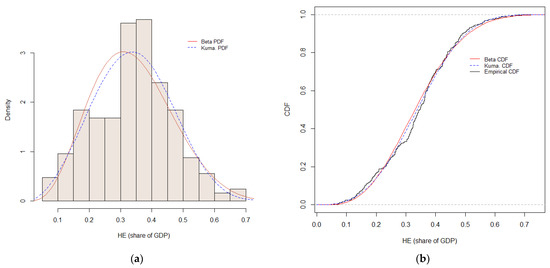
Figure 3. (a) Hidden economy densities. (b) Distribution functions.

4.2. Food Expenditure

The second application uses data for the fraction of household income that is spent on food. A random sample of 38 households is available in the “FoodExpenditure” data-set in the ‘betareg’ package for R (Zeileis et al. [40]). In our sample, the observations range from 0.1075 to 0.5612 in value, and the sample mean and standard deviation are 0.2897 and 0.1014, respectively. When a Kumaraswamy distribution is fitted to the data, the estimates of the two shape parameters are 2.9546 and 26.9653. See Figure 4a,b. The Anderson–Darling statistic is 0.8521, which exceeds the asymptotic and simulated 5% critical values of 0.7520 and 0.7415, respectively. This supports the rejection of the hypothesis that the data are Kumaraswamy-distributed. Fitting a beta distribution to the data yields estimates of 6.0721 and 14.8224 for the shape parameters. The corresponding Anderson–Darling statistic is 0.5114. The asymptotic and simulated 5% critical values are 0.7520 and 0.7700, respectively, suggesting that the hypothesis that the data are beta-distributed cannot be rejected at this significance level.

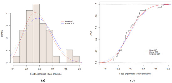
Figure 4. (a) Food expenditure densities. (b) Distribution functions.

5. Conclusions

The Kumaraswamy distribution is an alternative to the beta distribution, which has been applied in statistical studies in a wide range of disciplines. Its theoretical properties are well established, but the literature lacks a discussion of formal goodness-of-fit tests for this distribution. In this paper, we have applied the “biased transformation” methodology suggested by Raschke [18] to various standard tests based on the empirical distribution function and investigated their performance for the Kumaraswamy distribution.

The results of our simulation experiment, which focuses on both the size and power of these tests, can be summarized as follows. The “biased transformation” EDF goodness-of-fit testing strategy performs well for the Kumaraswamy distribution against a wide range of possible alternatives, though it needs to be treated with caution against certain beta distribution alternatives. In all cases, the Anderson–Darling test clearly emerges as the most powerful test of those considered and is recommended for practitioners.

References

- Kumaraswamy, P. A generalized probability density function for double-bounded random processes. J. Hydrol. 1980, 46, 79–88. [Google Scholar] [CrossRef]
- Sundar, V.; Subbiah, K. Application of double bounded probability density function for analysis of ocean waves. Ocean Eng. 1989, 16, 193–200. [Google Scholar] [CrossRef]
- Seifi, A.; Ponnambalam, K.; Vlach, J. Maximization of Manufacturing Yield of Systems with Arbitrary Distributions of Component Values. Ann. Oper. Res. 2000, 99, 373–383. [Google Scholar] [CrossRef]
- Ponnambalam, K.; Seifi, A.; Vlach, J. Probabilistic design of systems with general distributions of parameters. Int. J. Circuit Theory Appl. 2001, 29, 527–536. [Google Scholar] [CrossRef]
- Ganji, A.; Ponnambalam, K.; Khalili, D.; Karamouz, M. Grain yield reliability analysis with crop water demand uncertainty. Stoch. Environ. Res. Risk Assess. 2006, 20, 259–277. [Google Scholar] [CrossRef]
- Courard-Hauri, D. Using Monte Carlo analysis to investigate the relationship between overconsumption and uncertain access to one’s personal utility function. Ecol. Econ. 2007, 64, 152–162. [Google Scholar] [CrossRef]
- Cordeiro, G.M.; Castro, M. A new family of generalized distributions. J. Stat. Comput. Simul. 2010, 81, 883–898. [Google Scholar] [CrossRef]
- Bayer, F.M.; Bayer, D.M.; Pumi, G. Kumaraswamy autoregressive moving average models for double bounded environmental data. J. Hydrol. 2017, 555, 385–396. [Google Scholar] [CrossRef]
- Cordeiro, G.M.; Machado, E.C.; Botter, D.A.; Sandoval, M.C. The Kumaraswamy normal linear regression model with applications. Commun. Stat.-Simul. Comput. 2018, 47, 3062–3082. [Google Scholar] [CrossRef]
- Nadarajah, S. On the distribution of Kumaraswamy. J. Hydrol. 2008, 348, 568–569. [Google Scholar] [CrossRef]
- McDonald, J.B. Some Generalized Functions for the Size Distribution of Income. Econometrica 1984, 52, 647. [Google Scholar] [CrossRef]
- Jones, M. Kumaraswamy’s distribution: A beta-type distribution with some tractability advantages. Stat. Methodol. 2009, 6, 70–81. [Google Scholar] [CrossRef]
- Garg, M. On Distribution of Order Statistics from Kumaraswamy Distribution. Kyungpook Math. J. 2008, 48, 411–417. [Google Scholar] [CrossRef]
- Mitnik, P.A. New properties of the Kumaraswamy distribution. Commun. Stat.-Theory Methods 2013, 42, 741–755. [Google Scholar] [CrossRef]
- Ferrari, S.; Cribari-Neto, F. Beta Regression for Modelling Rates and Proportions. J. Appl. Stat. 2004, 31, 799–815. [Google Scholar] [CrossRef]
- Mitnik, P.A.; Baek, S. The Kumaraswamy distribution: Median-dispersion re-parameterizations for regression modeling and simulation-based estimation. Stat. Pap. 2013, 54, 177–192. [Google Scholar] [CrossRef]
- Hamedi-Shahraki, S.; Rasekhi, A.; Yekaninejad, M.S.; Eshraghian, M.R.; Pakpour, A.H. Kumaraswamy regression modeling for Bounded Outcome Scores. Pak. J. Stat. Oper. Res. 2021, 17, 79–88. [Google Scholar] [CrossRef]
- Raschke, M. The Biased Transformation and Its Application in Goodness-of-Fit Tests for the Beta and Gamma Distribution. Commun. Stat.-Simul. Comput. 2009, 38, 1870–1890. [Google Scholar] [CrossRef]
- Anderson, T.W.; Darling, D.A. Asymptotic theory of certain “goodness of fit” criteria based on stochastic processes. Ann. Math. Stat. 1952, 23, 193–212. [Google Scholar] [CrossRef]
- Anderson, T.W.; Darling, D.A. A test for goodness of fit. J. Am. Stat. Assoc. 1954, 49, 300–310. [Google Scholar] [CrossRef]
- Raschke, M. Empirical behaviour of tests for the beta distribution and their application in environmental research. Stoch. Environ. Res. Risk Assess. 2011, 25, 79–89. [Google Scholar] [CrossRef]
- Kuiper, N.H. Tests concerning random points on a circle. Proc. K. Ned. Akad. Wet. A 1962, 63, 38–47. [Google Scholar] [CrossRef]
- Watson, G.S. Goodness-of-fit tests on a circle. I. Biometrika 1961, 48, 109–114. [Google Scholar] [CrossRef]
- Cramér, H. On the composition of elementary errors. Scand. Actuar. J. 1928, 1928, 13–74. [Google Scholar] [CrossRef]
- von Mises, R.E. Wahrscheinlichkeit, Statistik und Wahrheit; Julius Springer: Vienna, Austria, 1928. [Google Scholar]
- Kolmogorov, A. Sulla determinazione empirica di una legge di distribuzione. G. dell’Ist. Ital. Attuari 1933, 4, 83–91. [Google Scholar]
- Smirnov, N. Table for Estimating the Goodness of Fit of Empirical Distributions. Ann. Math. Stat. 1948, 19, 279–281. [Google Scholar] [CrossRef]
- Lemonte, A.J. Improved point estimation for the Kumaraswamy distribution. J. Stat. Comput. Simul. 2011, 81, 1971–1982. [Google Scholar] [CrossRef]
- Stephens, M.A. Tests based on EDF statistics. In Goodness-of-Fit Techniques; D’Augustino, R.B., Stephens, M.A., Eds.; Marcel Dekker: New York, NY, USA, 1986; pp. 97–194. [Google Scholar]
- R Core Team. R: A Language and Environment for Statistical Computing; R Foundation for Statistical Computing: Vienna, Austria, 2024; Available online: https://www.R-project.org/ (accessed on 5 March 2024).
- Moss, J.; Nagler, T. Package ‘univariateML’. 2022. Available online: https://cran.r-project.org/web/packages/univariateML/univariateML.pdf (accessed on 5 March 2024).
- Pavia, J.M. Package ‘GoFKernel’. 2022. Available online: https://cran.r-project.org/web/packages/GoFKernel/GoFKernel.pdf (accessed on 5 March 2024).
- Millard, S.P.; Kowarik, A. Package ‘EnvStats’. 2023. Available online: https://cran.r-project.org/web/packages/EnvStats/EnvStats.pdf (accessed on 5 March 2024).
- Yee, T. Package ‘VGAM’. 2023. Available online: https://cran.r-project.org/web/packages/VGAM/VGAM.pdf (accessed on 5 March 2024).
- Hetzel, J.T. Package ‘trapezoid’. 2022. Available online: https://cran.r-project.org/web/packages/trapezoid/trapezoid.pdf (accessed on 5 March 2024).
- Mersmann, O.; Trautmann, H.; Steuer, D.; Bornkamp, B. Package ‘Truncnorm’. 2023. Available online: https://cran.r-project.org/web/packages/truncnorm/truncnorm.pdf (accessed on 5 March 2024).
- Bear, R.; Shang, K.; You, H.; Fannin, B. Package ‘Cascsim’. 2022. Available online: https://cran.r-project.org/web/packages/cascsim/cascsim.pdf (accessed on 5 March 2024).
- Reynkens, T. Package ‘ReIns’. 2023. Available online: https://cran.r-project.org/web/packages/ReIns/ReIns.pdf (accessed on 5 March 2024).
- Medina, L.; Schneider, H. Shedding Light on the Shadow Economy: A Global Database and the Interaction with the Official One; CESifo Working Paper No. 7981; Ludwig Maximilian University of Munich: Munich, Germany, 2019. [Google Scholar] [CrossRef]
- Zeileis, A.; Cribari-Neto, F.; Gruen, B.; Kosmidis, I.; Simas, A.B.; Rocha, A.V. Package ‘betareg’. 2022. Available online: https://cran.r-project.org/web/packages/betareg/betareg.pdf (accessed on 5 March 2024).
Disclaimer/Publisher’s Note: The statements, opinions and data contained in all publications are solely those of the individual author(s) and contributor(s) and not of MDPI and/or the editor(s). MDPI and/or the editor(s) disclaim responsibility for any injury to people or property resulting from any ideas, methods, instructions or products referred to in the content. |
© 2024 by the author. Licensee MDPI, Basel, Switzerland. This article is an open access article distributed under the terms and conditions of the Creative Commons Attribution (CC BY) license (https://creativecommons.org/licenses/by/4.0/).