Revisiting the Large n (Sample Size) Problem: How to Avert Spurious Significance Results

Abstract

Although large data sets are generally viewed as advantageous for their ability to provide more precise and reliable evidence, it is often overlooked that these benefits are contingent upon certain conditions being met. The primary condition is the approximate validity (statistical adequacy) of the probabilistic assumptions comprising the statistical model ${\mathcal{M}}_{\mathit{\theta }}\left(\mathbf{x}\right)$ applied to the data. In the case of a statistically adequate ${\mathcal{M}}_{\mathit{\theta }}\left(\mathbf{x}\right)$ and a given significance level $\alpha$, as n increases, the power of a test increases, and the p-value decreases due to the inherent trade-off between type I and type II error probabilities in frequentist testing. This trade-off raises concerns about the reliability of declaring ‘statistical significance’ based on conventional significance levels when n is exceptionally large. To address this issue, the author proposes that a principled approach, in the form of post-data severity (SEV) evaluation, be employed. The SEV evaluation represents a post-data error probability that converts unduly data-specific ‘accept/reject $H_0$ results’ into evidence either supporting or contradicting inferential claims regarding the parameters of interest. This approach offers a more nuanced and robust perspective in navigating the challenges posed by the large n problem.

1. Introduction

The recent availability of big data with large sample sizes (n) in many scientific disciplines brought to the surface an old and largely forgotten foundational issue in frequentist testing known as the ‘large n problem’. It relates to inferring that an estimated parameter is statistically significant based on conventional thresholds, $\alpha =0.1,0.05,0.025,0.01$, when n is very large, say $n>100,000$.

1.1. A Brief History of the Large n Problem

As early as 1938, Berkson [1] brought up the large n problem by pointing out its effect on the p-value:

“… when the numbers in the data are quite large, the P’s [p-values] tend to come out small… if the number of observations is extremely large—for instance, on the order of 200,000—the chi-square P will be small beyond any usual limit of significance. … If, then, we know in advance the P that will result…, it is no test at all. ”

(p. 527)

In 1935 Fisher [2] pinpointed the effect of the large n problem on the power (he used the term sensitivity) of the test:

“By increasing the size of the experiment [n], we can render it more sensitive, meaning by this that it will allow of the detection of … quantitatively smaller departures from the null hypothesis.”

(pp. 21–22)

In 1942 Berkson [3] returned to the large n problem by arguing that it also affects the power of a test, rendering it relevant for a sound evidential interpretation:

“In terms of the Neyman–Pearson (N-P) formulation they have different powers for any particular alternative, and hence are likely to give different results in any particular case. ”

(p. 334)

One of the examples he uses to make his case is from Fisher’s book [4] which is about testing the linearity assumption of a Linear Regression (LR) model.

Unfortunately, the example allowed Fisher [5] to brush aside the broader issues of misinterpreting frequentist tests as evidence for or against hypotheses. In his response, he focuses narrowly on the particular example and recasts their different perspectives on frequentist testing as a choice between ‘objective tests of significance’ and ‘subjective impressions based on eyeballing’ a scatterplot:

“He has drawn the graph. He has applied his statistical insight and his biological experience to its interpretation. He enunciates his conclusion that ‘on inspection it appears as straight a line as one can expect to find in biological material.’ The fact that an objective test had demonstrated that the departure from linearity was most decidedly significant is, in view of the confidence which Dr. Berkson places upon subjective impressions, taken to be evidence that the test of significance was misleading, and therefore worthless.”

(p. 692)

In his reply, Berkson [6], (p. 243), reiterated the role of the power:

“When with such specific tests one has sufficient numbers, they become sensitive tests; in the terminology of Neyman and Pearson they become ‘powerful’. ”

As a result of the exchange between Berkson and Fisher, the broader issue of ‘inference results’ vs. ‘evidence’ was put aside by the statistics literature until the late 1950s. Berkson’s example from Fisher [4] was an unfortunate choice since the test in question is not a N-P type test, which probes within the boundaries of the invoked statistical model, ${\mathcal{M}}_{\mathit{\theta }}\left(\mathbf{x}\right)$, by framing the hypotheses of interest in terms of its unknown parameters $\mathit{\theta }$. It is a misspecification test, which probes outside the boundaries of ${\mathcal{M}}_{\mathit{\theta }}\left(\mathbf{x}\right)$ to evaluate the validity of its assumptions—the linearity in this case; see Spanos [7].

In 1957 Lindley [8] presented the large n problem as a conflict between frequentist and Bayesian testing by arguing that the p-value will reject $H_0$: $\theta ={\theta }_0$ as n increases, whereas the Bayes factor will favor $H_0$. Subsequently, this became known as the Jeffreys–Lindley paradox (Spanos [9]) for further discussion.

In 1958 Lehmann [10] raised the issue of the sample size influencing the power of a test, and proposed decreasing $\alpha$ as n increases to counter-balance the increase in its power:

“By habit, and because of the convenience of standardization in providing a common frame of reference, these values [$\alpha =0.1,0.05,0.025,0.01$] became entrenched as conventional levels to use. This is unfortunate since the choice of significance level should also take into consideration the power that the test will achieve against alternatives of interest. There is little point in carrying out an experiment that has only a small chance of detecting the effect being sought when it exists. Surveys by Cohen [11] and Freiman et al. [12] suggest that this is, in fact, the case for many studies. ”

(Lehmann [13], pp. 69–70)

Interestingly, the papers cited by Lehmann [13] have been published in psychology and medical journals, respectively, indicating that practitioners in certain disciplines became aware of the small/large n problems and began exploring solutions. Cohen [11,14], was particularly influential in convincing psychologists to supplement, or even replace the p-value, with a statistic that is free of n, known as the ‘effect size’, to address the large n problem. For instance, Cohen’s $d=\frac{({\overline{x}}_n-{\overline{y}}_n)}{s}$ is the recommended effect size when one is testing the difference between two means based on the test statistic $\frac{\sqrt{N}[({\overline{X}}_n-{\overline{Y}}_n)-\gamma ]}{s}$ in testing $H_0$: $\gamma =0$ vs. $H_1$: $\gamma \ne 0;$ see Lehmann [13].

In 1982 Good [15], p. 66, went a step further than Lehmann [10] to propose a rule of thumb: “p-values … should be standardized to a fixed sample size, say N = 100, by replacing P [$p_n\left({\mathbf{x}}_0\right)$] with $min\left(0.5,\left[p_n\left({\mathbf{x}}_0\right)·\sqrt{n/100}\right]\right),n>10.$ ”

1.2. Large n Data and the Preconditions for More Accurate and Trustworthy Evidence

Large n data are universally considered a blessing since they can potentially give rise to more accurate and trustworthy evidence. What is often neglected, however, is that the potential for such gains requires certain ‘modeling’ and ‘inference’ stipulations to be met before any such accurate and trustworthy evidence can materialize.

[a] The most crucial modeling stipulation is for the practitioner to establish the statistical adequacy (approximate validity) of the invoked probabilistic assumptions imposed on one’s data, say ${\mathbf{x}}_0:$= $(x_1,x_2,...,x_n),$ comprising the relevant statistical model ${\mathcal{M}}_{\mathit{\theta }}\left(\mathbf{x}\right)$; see Spanos [16]. Invalid probabilistic assumptions induce sizeable discrepancies between the nominal error probabilities—derived assuming the validity of ${\mathcal{M}}_{\mathit{\theta }}\left(\mathbf{x}\right)$—and the actual ones based on ${\mathbf{x}}_0$, rendering the inferences unreliable and the ensuing evidence untrustworthy. Applying a $0.05$ significance level test when the actual type I error probability is closer to $0.97,$ due to invalid probabilistic assumptions (Spanos [17], p. 691) will yield spurious inference results and untrustworthy evidence; see Spanos [18] for additional examples.

[b] The most crucial inference stipulation for the practitioner is to distinguish between raw ‘inference results’, such as point estimates, effect sizes, observed CIs, ‘accept/reject $H_0$’, and p-values, and ‘evidence for or against inferential claims’ relating to unknown parameters $\mathit{\theta }$. Conflating the two often gives rise to fallacious evidential interpretations of such inference results, as well as unwarranted claims, including spurious statistical significance with a large n. The essential difference between ‘inference results’ and ‘evidence’ is that the former rely unduly on the particular data ${\mathbf{x}}_0:=(x_1,x_2,...,x_n),$ which constitutes a single realization $\mathbf{X}={\mathbf{x}}_0$ of the sample $\mathbf{X}:=(X_1,...,X_n)$. In contrast, sound evidence for or against inferential claims relating to $\mathit{\theta }$ needs to account for that uncertainty.

The main objective of the paper is to make a case that the large n problem can be addressed using a principled argument based on the post-data severity (SEV) evaluation of the unduly data-specific accept/reject results. This is achieved by accounting for the inference-related uncertainty to provide an evidential interpretation of such results that revolves around the discrepancy $\gamma \ne 0$ from the null value warranted by the particular test and data ${\mathbf{x}}_0$ with high enough post-data error probability. This provides an inductive generalization of the accept/reject results that enhances learning from data.

As a prelude to the discussion that follows, Section 2 summarizes Fisher’s [19] model-based frequentist statistics, with particular emphasis on Neyman–Pearson (N-P) testing. Section 3 considers the large n problem and its implications for the p-value and the power of an N-P test. Section 4 discusses examples from the empirical literature in microeconometrics where the large n problem is largely ignored. Section 5 explains how the post-data severity evaluation of the accept/reject $H_0$ results can address the large n problem and is illustrated using hypothetical and actual data examples.

2. Model-Based Frequentist Statistics: An Overview

2.1. Fisher’s Model-Based Statistical Induction

Model-based frequentist statistics was pioneered by Fisher [19] in the form of statistical induction that revolves around a statistical model whose generic form is:

$$\begin{array}{c}{\mathcal{M}}_{\mathit{\theta }}\left(\mathbf{x}\right)=\{f(\mathbf{x};\mathit{\theta }),\mathit{\theta }\in \mathrm{\Theta }\},\mathbf{x}\in {\mathbb{R}}_X^n,\mathrm{for}\mathrm{\Theta }\subset {\mathbb{R}}^m,m<n,\end{array}$$

(1)

and revolves around the distribution of the sample $\mathbf{X}:=(X_1,X_2,...,X_n),$ $f(\mathbf{x};\mathit{\theta }),\mathbf{x}\in {\mathbb{R}}_X^n,$ $\mathbb{R}:=(-\infty ,\infty )$, which encapsulates its probabilistic assumptions. ${\mathbb{R}}_X^n$ denotes the sample space, and $\mathrm{\Theta }$ the parameter space; see Spanos [16].

Unfortunately, the term ‘model’ is used to describe many different constructs across different disciplines. In the context of empirical modeling using statistics, however, the relevant models can be grouped into two broad categories: ‘substantive’ (structural, a priori postulated) and ‘statistical’ models. Although these two categories of models are often conflated, a statistical model ${\mathcal{M}}_{\mathit{\theta }}\left(\mathbf{x}\right)$ comprises solely the probabilistic assumptions imposed (explicitly or implicitly) on the particular data ${\mathbf{x}}_0$; see McCullagh [20]. Formally, ${\mathcal{M}}_{\mathit{\theta }}\left(\mathbf{x}\right)$ is a stochastic mechanism framed in terms of probabilistic assumptions from three broad categories: Distribution (D), Dependence (M), and Heterogeneity (H), assigned to the observable stochastic process $\{X_t,t\in \mathbb{N}:=(1,2,...,n,...)\}$ underlying data ${\mathbf{x}}_0$.

The specification (initial selection) of ${\mathcal{M}}_{\mathit{\theta }}\left(\mathbf{x}\right)$ has a twofold objective:

(a)

${\mathcal{M}}_{\mathit{\theta }}\left(\mathbf{x}\right)$ is selected to account for all the chance regularity patterns—the systematic statistical information—in data ${\mathbf{x}}_0$ by choosing appropriate probabilistic assumptions relating to $\{X_k,k\in \mathbb{N}\}$. Equivalently, ${\mathcal{M}}_{\mathit{\theta }}\left(\mathbf{x}\right)$ is selected to render data ${\mathbf{x}}_0$ a ‘typical realization’ therefrom, and the ‘typicality’ can be evaluated using Mis-Specification (M-S) testing, which evaluates the approximate validity of its probabilistic assumptions.

(b)

${\mathcal{M}}_{\mathit{\theta }}\left(\mathbf{x}\right)$ is parametrized [$\mathit{\theta }\in \mathrm{\Theta }$] to enable one to shed light on the substantive questions of interest using data ${\mathbf{x}}_0$. When these questions are framed in terms of a substantive model, say ${\mathcal{M}}_{\mathit{\phi }}\left(\mathbf{x}\right),$$\mathit{\phi }\in \mathrm{\Phi }$, one needs to bring out the implicit statistical model in a way that ensures that the two sets of parameters are related via a set of restrictions $g\left(\mathit{\phi },\mathit{\theta }\right)=0$ colligating $\mathit{\phi }$ to the data ${\mathbf{x}}_0$ via $\mathit{\theta }$; see Spanos [16].

Example 1. A widely used example in practice is the simple Normal model:

$$\begin{array}{cc}{\mathcal{M}}_{\mathit{\theta }}\left(\mathbf{x}\right):& X_t\backsim \mathsf{NIID}(\mu ,{\sigma }^2),(\mu ,{\sigma }^2)\in \mathbb{R}\times {\mathbb{R}}_{+},x_t\in \mathbb{R},t\in \mathbb{N},\end{array}$$

(2)

where ‘$\mathsf{NIID}$’ stands for ‘Normal (D), Independent (M), and Identically Distributed (H)’.

The main objective of the model-based frequentist inference is to ‘learn from data ${\mathbf{x}}_0$’ about ${\mathit{\theta }}^{*},$ where ${\mathit{\theta }}^{*}$ denotes the ‘true’ value of $\mathit{\theta }$ in $\mathrm{\Theta }$; shorthand for saying that there exists a ${\mathit{\theta }}^{*}\in \mathrm{\Theta }$ such that ${\mathcal{M}}^{*}\left(\mathbf{x}\right)=f\left({x;\mathit{\theta }}^{*}\right),\mathbf{x}\in {\mathbb{R}}_X^n,$ could have generated data ${\mathbf{x}}_0$.

The cornerstone of frequentist inference is the concept of a sampling distribution, $f(y_n;\mathit{\theta })=d{F}_n\left(y\right)/dy,$ for all (∀) $y\in {\mathbb{R}}_Y$, of a statistic $Y_n=g(X_1,X_2,...,X_n)$ (estimator, test, predictor), derived via:

$$\begin{array}{c}{F}_n\left(y\right)=\mathbb{P}(Y_n\le y)=\underset{\{\mathbf{x}:g(\mathbf{x})\le y\}}{\underbrace{\int \int \cdots \int }}f(\mathbf{x};\mathit{\theta })d\mathbf{x},\forall y\in {\mathbb{R}}_Y.\end{array}$$

(3)

The derivation of $f(y_n;\mathit{\theta }),\forall y\in {\mathbb{R}}_Y,$ in (3) presumes the validity of $f(\mathbf{x};\mathit{\theta }),\mathbf{x}\in {\mathbb{R}}_X^n,$ which in the case of (2) is: $\begin{array}{c}f(\mathbf{x};\mathit{\theta })\stackrel{\mathrm{NIID}}{=}{\left(\frac{1}{\sqrt{2\pi {\sigma }^2}}\right)}^{n}exp\{-\frac{1}{2{\sigma }^2}{\sum }_{k=1}^n{(x_k-\mu )}^2\},\mathbf{x}\in {\mathbb{R}}^n.\end{array}$

In light of the crucial role of the distribution of the sample, Fisher [19], p. 314, emphasized the importance of establishing the statistical adequacy (approximate validity) of the invoked statistical model ${\mathcal{M}}_{\mathit{\theta }}\left(\mathbf{x}\right)$:

“For empirical as the specification of the hypothetical population [${\mathcal{M}}_{\mathit{\theta }}\left(\mathbf{x}\right)$] may be, this empiricism is cleared of its dangers if we can apply a rigorous and objective test of the adequacy with which the proposed population represents the whole of the available facts.”

He went on to underscore the crucial importance of Mis-Specification (M-S) testing (testing the approximate validity of the probabilistic assumptions comprising ${\mathcal{M}}_{\mathit{\theta }}\left(\mathbf{x}\right)$) as the way to provide an empirical justification for statistical induction:

“The possibility of developing complete and self-contained tests of goodness of fit deserves very careful consideration, since therein lies our justification for the free use which is made of empirical frequency formulae. ”

(Fisher [19], (p. 314).)

Statistical adequacy plays a crucial role in securing the reliability of inference because it ensures the approximate equality between the actual and the nominal error probabilities based on ${\mathbf{x}}_0,$ assuring that one can keep track of the relevant error probabilities. In contrast, when ${\mathcal{M}}_{\mathit{\theta }}\left(\mathbf{x}\right)$ is statistically misspecified (Spanos, [21]),

(a)

$f(\mathbf{x};\mathit{\theta }),\mathbf{x}\in {\mathbb{R}}_X^n,$ and the likelihood function $L({\mathbf{x}}_0;\mathit{\theta })\propto f({\mathbf{x}}_0;\mathit{\theta }),\forall \mathit{\theta }\in \mathrm{\Theta }$ are erroneous,

(b)

distorting the sampling distribution $f(y_n;\mathit{\theta })$ derived via (3), as well as

(c)

giving rise to ‘non-optimal’ estimators and sizeable discrepancies between the actual error probabilities and nominal—derived assuming ${\mathcal{M}}_{\mathit{\theta }}\left(\mathbf{x}\right)$ is valid.

In light of that, the practical way to keep track of the relevant error probabilities is to establish the statistical adequacy of ${\mathcal{M}}_{\mathit{\theta }}\left(\mathbf{x}\right)$. When ${\mathcal{M}}_{\mathit{\theta }}\left(\mathbf{x}\right)$ is misspecified, any attempt to adjust the relevant error probabilities is ill-fated because the actual error probabilities are unknown due to being sizeably different from the nominal ones.

Regrettably, as Rao [22], p. 2, points out, validating ${\mathcal{M}}_{\mathit{\theta }}\left(\mathbf{x}\right)$ using comprehensive M-S testing is neglected in statistics courses:

“They teach statistics as a deductive discipline of deriving consequences from given premises [${\mathcal{M}}_{\mathit{\theta }}\left(\mathbf{x}\right)$]. The need for examining the premises, which is important for practical applications of results of data analysis is seldom emphasized. … The current statistical methodology is mostly model-based, without any specific rules for model selection or validating a specified model. ”

(p. 2)

See Spanos [23] for further discussion.

2.2. Neyman–Pearson (N-P) Testing

Example 1 (continued). In the context of (2), testing the hypotheses:

$$\begin{array}{c}{H}_0:\mu \le {\mu }_0\mathrm{vs}.H_1:\mu >{\mu }_0,\end{array}$$

(4)

an optimal (UMP) $\alpha$-significance level test (Neyman and Pearson, 1933 [24]) is:

$$\begin{array}{c}{T}_{\alpha }:=[\tau \left(\mathbf{X}\right)=\frac{\sqrt{n}({\overline{X}}_n-{\mu }_0)}{s},C_1\left(\alpha \right)=\{\mathbf{x}:\tau \left(\mathbf{x}\right)>c_{\alpha }\}],\end{array}$$

(5)

where ${\overline{X}}_n=\frac{1}{n}{\sum }_{k=1}^n{X}_k,s_n^2=\frac{1}{(n-1)}{\sum }_{k=1}^n{(X_k-{\overline{X}}_n)}^2,$ $C_1\left(\alpha \right)$ denotes the rejection region, and $c_{\alpha }$ is determined by the significance level $\alpha$; see Lehmann [13].

The sampling distribution of $\tau \left(\mathbf{X}\right)$ evaluated under $H_0$ (hypothetical) is:

$$\begin{array}{c}\tau \left(\mathbf{X}\right)=\frac{\sqrt{n}({\overline{X}}_n-{\mu }_0)}{s}\stackrel{\mu ={\mu }_0}{\backsim }\mathsf{St}(n-1),\end{array}$$

(6)

where ‘$\mathsf{St}(n-1)$’ denotes the Student’s t distribution with $(n-1)$ degrees of freedom, which provides the basis for evaluating the type I error probability and the p-value:

$$\begin{array}{cc}\alpha =\mathbb{P}(\tau \left(\mathbf{X}\right)>c_{\alpha };\mu ={\mu }_0),\hfill & p\left({\mathbf{x}}_0\right)=\mathbb{P}(\tau \left(\mathbf{X}\right)>\tau \left({\mathbf{x}}_0\right);\mu ={\mu }_0).\hfill \end{array}$$

(7)

That is, both the type I error probability and the p-value in (7) are evaluated using hypothetical reasoning, that interprets ‘$\mu ={\mu }_0$ is true’ as ‘what if’ ${\mu }_0={\mu }^{*}$’.

The sampling distribution of $\tau \left(\mathbf{X}\right)$ evaluated under $H_1$ (hypothetical) is:

$$\begin{array}{c}\tau \left(\mathbf{X}\right)=\frac{\sqrt{n}\left({\overline{X}}_n-{\mu }_0\right)}{\sigma }\stackrel{\mu ={\mu }_1}{\backsim }\mathrm{St}({\delta }_1;n-1),{\delta }_1=\frac{\sqrt{n}\left({\mu }_1-{\mu }_0\right)}{\sigma },\forall {\mu }_1={\mu }_0+{\gamma }_1,{\gamma }_1\ge 0,\end{array}$$

(8)

where ${\delta }_1$ is the noncentrality parameter of St$({\delta }_1;n-1)$, which provides the basis for evaluating the power of test $T_{\alpha }$:

$$\begin{array}{c}\mathcal{P}\left({\mu }_1\right)=\mathbb{P}(\tau \left(\mathbf{X}\right)>c_{\alpha };\mu ={\mu }_1),\forall {\mu }_1={\mu }_0+{\gamma }_1,{\gamma }_1\ge 0.\end{array}$$

(9)

where ${\delta }_1=\frac{\sqrt{n}\left({\mu }_1-{\mu }_0\right)}{\sigma }$ in (8) indicates that the power increases monotonically with $\sqrt{n}$ and $\left({\mu }_1-{\mu }_0\right)$ and decreases with $\sigma$.

$$\begin{array}{c}\mathcal{P}\left({\mu }_1\right)=\mathbb{P}(\tau \left(\mathbf{X}\right)>c_{\alpha };\mu ={\mu }_1),\forall {\mu }_1={\mu }_0+{\gamma }_1,{\gamma }_1\ge 0.\end{array}$$

(10)

Equation (8) shows that the power increases with $\sqrt{n}$ and $\left({\mu }_1-{\mu }_0\right)$ and decreases with $\sigma$.

The optimality of N-P tests revolves around an inherent trade-off between the type I and II error probabilities. To address that trade-off, Neyman and Pearson [24] proposed to construct an optimal test by prespecifying $\alpha$ at a low value and minimizing the type II error $\beta \left({\mu }_1\right)$, or maximizing the power $\mathcal{P}\left({\mu }_1\right)=(1-\beta \left({\mu }_1\right))$, $\forall {\mu }_1={\mu }_0+{\gamma }_1,{\gamma }_1\ge 0$.

A question that is often overlooked in traditional expositions of N-P testing is:

Where does prespecifying the type I error probability at a low threshold come from?

A careful reading of Neyman and Pearson [24] reveals the answer in the form of two crucial stipulations relating to the framing of $H_0$: $\theta \in {\mathrm{\Theta }}_0$ and $H_1$: $\theta \in {\mathrm{\Theta }}_1,$ to ensure the effectiveness of N-P testing and the informativeness of the ensuing results:

• ${\mathrm{\Theta }}_0$ and ${\mathrm{\Theta }}_1$ should form a partition of $\mathrm{\Theta }$ (p. 293) to avoid ${\theta }^{*}\notin [{\mathrm{\Theta }}_0\cup {\mathrm{\Theta }}_1].$
• ${\mathrm{\Theta }}_0$ and ${\mathrm{\Theta }}_1$ should be framed in such a way to ensure that the type I error is the more serious of the two, using the analogy with a criminal trial, p. 296, with $H_0$: no guilty, to secure a low probability for sending an innocent person to jail.

Unveiling the intended objective of stipulation 2, suggests that the requirement for a small (prespecified) $\alpha$ is to ensure that the test has a low probability of rejecting a true null hypothesis, i.e., when ${\theta }_0={\theta }^{*}.$ Minimizing the type II error probability implies that an optimal test should have the lowest possible probability (or equivalently, the highest power) for accepting (rejecting) $\theta ={\theta }_0,$ when false, i.e., when ${\theta }_0\ne {\theta }^{*}$. That is, an optimal test should have a high power around the potential neighborhood of ${\theta }^{*}.$ This implies that when no reliable information about this potential neighborhood is available, one should use a two-sided test to avert the case where the test has no or very low power around ${\theta }^{*}$; see Spanos [25].

For the reason that the power increases with n, it is important to take that into account in selecting an appropriate $\alpha$ to avoid both an under-powered and an over-powered test, forefending the ‘small n’ and ‘large n problems’, respectively. First, for a given $\alpha$, one needs to calculate the value of n needed for $T_{\alpha }$ to have sufficient power to detect parameter discrepancies $\gamma \ne 0$ of interest; see Spanos [26]. Second, for a large n one needs to adjust $\alpha$ to avoid an ultra-sensitive test that could detect tiny discrepancies, say $\gamma =0.0000001$, and misleadingly declare them statistically significant.

The primary role of the pre-data testing error probabilities (type I, II, and power) is to operationalize the notions of ‘statistically significant/insignificant’ in terms of statistical approximations framed in terms of a test statistic $\tau \left(\mathbf{X}\right)$ and its sampling distribution. These error probabilities calibrate the capacity of the test to shed sufficient light on ${\theta }^{*}$, giving rise to learning from data. In this sense, the reliability of the testing results ‘accept/reject $H_0$’ depends crucially on the particular testing statistical context (Spanos, [17], ch. 13):

$$\begin{array}{c}\hfill \left(\mathrm{i}\right){\mathcal{M}}_{\mathit{\theta }}\left(\mathbf{x}\right),\left(\mathrm{i}\mathrm{i}\right)H_0:\theta \in {\mathrm{\Theta }}_0 \mathrm{v}\mathrm{s}. H_1:\theta \in {\mathrm{\Theta }}_1,\left(\mathrm{i}\mathrm{i}\mathrm{i}\right)T_{\alpha }:=\{d\left(\mathbf{X}\right),C_1\left(\alpha \right)\},\left(\mathrm{iv}\right) \mathrm{data} {\mathbf{x}}_0,\end{array}$$

(11)

which includes, not only the adequacy of ${\mathcal{M}}_{\mathit{\theta }}\left(\mathbf{x}\right)$ vis-a-vis data ${\mathbf{x}}_0$, the framing of $H_0$ and $H_1,$ and as well as n; see Spanos ([16,17]). For instance, when $n>10,000$, detaching the accept/reject $H_0$ results from their statistical context in (11), and claiming statistical significance at conventional thresholds will often be an unwarranted claim.

Let us elaborate on this assertion.

3. The Large $\mathbf{n}$ Problem in N-P Testing

3.1. How Could One Operationalize as n Increases?

As mentioned above, for a given $\alpha ,$ increasing n increases the test’s power and decreases the p-value. What is not so obvious is how to operationalize the clause ‘as n increases’ since data ${\mathbf{x}}_0$ usually come with a specific sample size n. Assuming that one begins with large enough n to ensure that the Mis-Specification (M-S) tests have sufficient power to detect existing departures from the probabilistic assumptions of the invoked ${\mathcal{M}}_{\mathit{\theta }}\left(\mathbf{x}\right)$, say $n=100,$ there are two potential scenarios one could contemplate.

Scenario 1 assumes that all different values of $n\ge 100$ give rise to the same observed $\tau \left({\mathbf{x}}_0\right)$. This scenario has been explored by Mayo and Spanos [27,28].

Scenario 2 assumes that as n increases beyond $n=100$ the change in the estimates ${\overline{x}}_n$ and $s_n^2$ are ‘relatively small’ to render the ratio $({\overline{x}}_n-{\mu }_0)/s_n$ approximately constant.

Scenario 2 seems realistic enough to shed light on the large n problem for two reasons. First, when the NIID assumptions are valid for ${\mathbf{x}}_n$, the changes in ${\overline{x}}_n$ and $s_n^2$ from increasing n are likely to be ‘relatively small’ since $n=100$ is sufficiently large to provide a reliable initial estimate, and thus, increasing n is unlikely to change the ratio drastically. Second, the estimate $({\overline{x}}_n-{\mu }_0)/s_n$ where ${\mu }_0$ is a value of interest, is known as the ‘effect size’ for $\mu$ in psychology (Ellis, [29]), and is often used to infer the magnitude of the ‘scientific’ effect, irrespective of n. Let us explore the effects of increasing n using scenario 2.

3.2. The Large n Problem and the p-Value

Empirical example 1 (continued). Consider the hypotheses in (4) for ${\mu }_0=2$ in the context of (2) using the following information:

$$\begin{array}{c}\hfill n=100,\alpha =0.05,c_{\alpha }=1.66,{\overline{x}}_n=2.317, \mathrm{and} s^2=3.7675(s=1.941).\end{array}$$

(12)

The test statistic $\tau \left(\mathbf{X}\right)=\frac{\sqrt{n}({\overline{X}}_n-{\mu }_0)}{s}$ yields:$\begin{array}{c}{\tau }_n\left({\mathbf{x}}_0\right)=\frac{\sqrt{100}(2.317-2)}{1.941}=1.6533,\end{array}$ with a p-value, $p_n\left({\mathbf{x}}_0\right)=0.0528,$ indicating ‘accept $H_0$’. The question of interest is how increasing n beyond $n=100$ will affect the result of N-P testing.

Consider the issue of how the p-value changes as n increases when $\frac{({\overline{x}}_n-{\mu }_0)}{s_n}$ is constant (scenario 2). The p-value curve in Figure 1 for $50<n\le 500$ indicates that one can manipulate n to obtain the desired result since (a) for $n<105$ the p-value will yield $p_n\left({\mathbf{x}}_0\right)>\alpha =0.05,$ ‘accept $H_0$’, (b) for $n>105$ the p-value will yield $p_n\left({\mathbf{x}}_0\right)<\alpha =0.05,$ ‘reject $H_0$’.

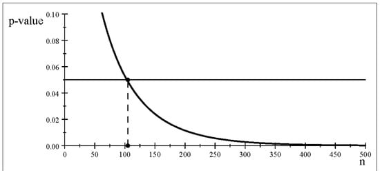
Figure 1. The p-value curve for different sample sizes n.

Table 1 reports particular values of ${\tau }_n\left({\mathbf{x}}_0\right)$ and $p_n\left({\mathbf{x}}_0\right)$ from Figure 1 as n increases, showing that $p_n\left({\mathbf{x}}_0\right)$ decreases rapidly down to tiny values for $n\ge 10,000$, confirming Berkson’s [1], (p. 334), observation in the introduction that the p-value “… will be small beyond any usual limit of significance. ”

Table 1. The p-value as n increases (keeping $({\overline{x}}_n-{\mu }_0)/s_n$ constant).

n	100	120	150	300	500	1000	2000	$10,000$
${\tau }_n\left({\mathbf{x}}_0\right)$	$1.633$	$1.789$	$2.0$	$2.829$	$3.652$	$5.165$	$7.304$	$16.332$
$p_n\left({\mathbf{x}}_0\right)$	$0.0528$	$0.038$	$0.024$	$0.0025$	$0.00014$	$0.00000015$	$0.2\times {10}^{-12}$	$0.0000...$

3.3. The Large n Problem and the Power of a Test

Let us consider the power of $T_{\alpha }^{>}$ at $0.8$ ($\mathbb{P}\left({\mu }_1\right)=0.8$) as n increases under scenario 2 ($({\overline{x}}_n-{\mu }_0)/s_n$ held constant), and evaluate its effect on the size of the detected discrepancies ${\gamma }_1={\mu }_1-{\mu }_0.$

Table 2 reports several values of n showing how the test detects smaller and smaller discrepancies from $\mu =2,$ confirming Fisher’s [2] quotation in the introduction. This can be seen more clearly in Figure 2, where the power curves become steeper and steeper as n increases.

Table 2. Discrepancy ${\gamma }_1$ detected with $P\left({\mu }_1\right)=0.8$ as n increases.

n	100	200	500	1000	$10,000$	$100,000$	$1,000,000$	$20,000,000$
${\gamma }_1$	$0.486$	$0.344$	$0.217$	$0.154$	$0.0485$	$0.01535$	$0.00486$	$0.0034$

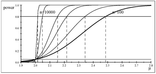
Figure 2. The power curve for different sample sizes n.

One might object to this quote as anachronistic since Fisher [30] was clearly against the use of the type II error probability and the power of a test due to his falsificationist stance where ‘accept $H_0$’ would not be an option. The response is that Fisher acknowledged the role of power using the term ‘sensitivity’ in the quotation (Section 1.1), as well as explicitly in Fisher [31], p. 295. Indeed, the presence of a rejection threshold $\alpha$ in Fisher’s significance testing brings into play the pre-data type I and II error probabilities, while his p-value is a post-data error probability; see Spanos [17].

4. The Empirical Literature and the Large $\mathbf{n}$ Problem

Examples of misuse of frequentist testing abound in all applied fields, but the large n problem is particularly serious in applied microeconometrics where very large sample sizes n are often employed to yield spurious significance results, which are then used to propose policy recommendations relating to relevant legislation; see Pesko and Warman [32].

4.1. Empirical Examples in Microeconometrics

Empirical example 2A (Abouk et al. [33], Appendix J: Table 1. p. 99). Based on an estimated LR model in (Table 7). with $n=24,730,930$, it is inferred that the estimates ${\widehat{\beta }}_k=0.004$, SE$\left({\widehat{\beta }}_k\right)=0.002,$ rendering the coefficient ${\beta }_k$ of a key variable $x_k$ statistically significant at $\alpha =0.05$.

Such empirical results and the claimed evidence based on the estimated models are vulnerable to three potential problems.

(i)

Statistical misspecification and the ensuing untrustworthy evidence since the discussion in the paper ignores the statistical adequacy of the estimated statistical models. Given that to evaluate the statistical adequacy of any published empirical study, one needs the original data to apply thorough misspecification testing (Spanos, [7]), that issue will be sidestepped in the discussion that follows.

(ii)

Large n problem. One of the many examples in the paper relates to the claimed statistical significance (with $n=24,730,930)$ at $\alpha =0.05$ of ${\beta }_k$, ignoring its potential ‘spurious’ statistical significance results stemming from the large n problem in N-P testing.

(iii)

Conflating ‘testing results’ with ‘evidence’. The authors claim evidence for ${\beta }_k\ne 0,$ and proceed to infer its implications for the effectiveness of different economic policies.

Empirical example 2A (continued). Abouk et al. [33] report ${\widehat{\beta }}_k=0.004$,

SE$\left({\widehat{\beta }}_k\right)=\sqrt{\frac{s}{n\sqrt{q_{kk}}}}=0.002,$ and $p\left({\mathbf{z}}_0\right)<0.05,$ implying:

$$\begin{array}{c}\hfill l\frac{\sqrt{n}({\widehat{\beta }}_k-0)}{s\sqrt{q_{kk}}}=\frac{\sqrt{24,730,930}\left(0.004\right)}{\sqrt{98.932}}=2, \mathrm{for} c_{0.025}=1.96 \mathrm{and} p\left({\mathbf{z}}_0\right)=0.045.\end{array}$$

The relevant sampling distribution of $\widehat{\mathit{\beta }}:=({\widehat{\beta }}_0,{\widehat{\mathit{\beta }}}_1)$ for the LR model is:

$$\begin{array}{c}(\sqrt{n}(\widehat{\mathit{\beta }}-\mathit{\beta })\mid \mathbf{X})\backsim \mathsf{N}(\mathbf{0},{\sigma }^2{\mathbf{Q}}_X^{-1}),\underset{n\to \infty }{lim}\left(\frac{{\mathbf{X}}^{\top }\mathbf{X}}{n}\right)={\mathbf{Q}}_X={\left[q_{ij}\right]}_{i,j=1}^m>0.\end{array}$$

Focusing on just one coefficient ${\beta }_k$ the t-test for its significance is:

$$\begin{array}{c}\tau \left(\mathbf{y}\right)=\frac{\sqrt{n}({\widehat{\beta }}_k-0)}{s/\sqrt{q_{kk}}}\stackrel{{\beta }_k=0}{\underset{n\to \infty }{\backsim }}\mathrm{N}(0,1),C_1\left(\alpha \right)=\{\mathbf{y}:\left|\tau \left(\mathbf{y}\right)\right|>c_{\frac{\alpha }{2}}\}.\end{array}$$

Using the information in example 2A, we can reconstruct what would $p_n\left({\mathbf{z}}_0\right)$ have been for different n using scenario 2. The results in Table 3 indicate that the authors’ claim of statistical significance (${\beta }_k\ne 0$) at $\alpha =0.05$ will be unwarranted for any $n<24,000,000$.

Table 3. The p-value with increasing n (constant estimates).

n	100	500	1000	2000	10,000	$10\times {10}^4$	$10\times {10}^5$	$20\times {10}^5$	$20\times {10}^6$	$24\times {10}^6$
${\tau }_n\left({\mathbf{x}}_0\right)$	0.004	0.009	0.0127	0.018	0.040	0.127	0.402	0.569	10.798	10.970
$p_n\left({\mathbf{x}}_0\right)$	0.997	0.993	0.990	0.986	0.967	0.899	0.688	0.570	0.072	0.049

Example 2B. Abouk et al. [33], Table 2, p. 57, report 42 ANOVA results for the difference between two means $({\overline{x}}_{n_1}-{\overline{y}}_{n_2})$, 40 of these tests have tiny p-values, less than $0.0000,$ even though the differences between the two means, $({\overline{x}}_{n_1}-{\overline{y}}_{n_2})$ appear to be very small. Surprisingly, two of the estimated differences are zero, $({\overline{x}}_{n_1}-{\overline{y}}_{n_2})=0$ (${\overline{x}}_{n_1}=13.2$, ${\overline{y}}_{n_2}=13.2$ and ${\overline{x}}_{n_1}=2.51$, ${\overline{y}}_{n_2}=2.51$), but their reported p-values are $0.8867$ and $0.0056$, respectively; one would have expected $p\left({\mathbf{z}}_0\right)=1$ when $\tau \left({\mathbf{z}}_0\right)=0.$ Looking at these results, one wonders what went wrong with the reported p-values.

The hypotheses of interest take the form (Lehmann, [13]):

$$\begin{array}{c}{H}_0:({\mu }_1-{\mu }_2)=0\mathrm{vs}.H_1:({\mu }_1-{\mu }_2)\ne 0\end{array}$$

with the optimal test being the t-test $T_{\alpha }^{\ne }=\{\tau \left(\mathbf{Z}\right),C_1=\{\mathbf{z}:$$\left|\tau \left(\mathbf{z}\right)\right|>c_{\frac{\alpha }{2}}\left\}\right\}$ where:

$$\begin{array}{c}\tau \left(\mathbf{Z}\right)=[\sqrt{N}({\overline{X}}_{n_1}-{\overline{Y}}_{n_2}-\gamma )/s_N]\stackrel{{\mu }_1-{\mu }_2=0}{\backsim }\mathsf{St}(n_1+n_2-2),N=\frac{n_1{n}_2}{n_1+n_2},\\ s_N^2=\frac{(n_1-1)s_1^2+(n_2-1)s_2^2}{(n_1+n_2-2)},s_1^2=\frac{1}{(n_1-1)}\sum _{i=1}^{n_1}{(X_i-{\overline{X}}_{n_1})}^2,s_2^2=\frac{1}{(n_2-1)}\sum _{i=1}^{n_2}{(Y_i-{\overline{Y}}_{n_2})}^2.\end{array}$$

(13)

A close look at this t-test suggests that the most plausible explanation for the above ‘strange results’ is the statistical software using (at least) 12-digit decimal precision. Given that the authors report mostly 3-digit estimates, the software is picking up tiny discrepancies, say $<0.0000001,$ which, when magnified by $\sqrt{N}$, could yield the reported p-values. That is, the reported results have (inadvertently) exposed the effect of the large n on the p-value.

4.2. Meliorating the Large n Problem Using Rules of Thumb

In light of the inherent trade-off between the type I and type II error probabilities, some statistics textbooks advise practitioners to use ‘rules of thumb’ based on decreasing $\alpha$ as n increases; see Lehmann [13].

• Ad hoc rules for adjusting $\alpha$ as n increases

$n=$	100	200	500	1000	10,000	20,000	200,000	⋯
$\alpha =$	0.05	0.025	0.01	0.001	0.0001	0.00001	0.00000001	⋯

2.

Good [15], p. 66, proposed to standardize the p-value $p_n\left({\mathbf{x}}_0\right)$ relative to $N=100.$

Applying his rule of thumb, $min\left(0.5,\left[p_n\left({\mathbf{x}}_0\right)·\sqrt{n/100}\right]\right),n>100,$ to the p-value curve in Figure 1, based on ${\tau }_n\left({\mathbf{x}}_0\right)=1.6533,$ yields:

$n=$	100	120	150	300	500	1000	5000	10,000
$p_n\left({\mathbf{x}}_0\right)=$	$0.0528$	$0.038$	$0.024$	$0.002$	$0.0002$	$0.000001$	$2.4\times {10}^{-20}$	$0.000...0$
$p_{100}\left({\mathbf{x}}_0\right)=$	$0.0528$	$0.042$	$0.029$	$0.0035$	$0.0045$	$0.000003$	$10.7\times {10}^{-19}$	$0.000...0$

The above numerical examples suggest that such rules of thumb for selecting $\alpha$ as n increases can meliorate the problem; they do not, however, address the large n problem since they are ad hoc, and their suggested thresholds decrease to nearly zero beyond $n=10,000$.

4.3. The Large n Problem and Effect Sizes

Although there is no authoritative definition of the notion of an effect size, the one that comes closest to its motivating objective is Thompson’s [34]:

“An effect size is a statistic quantifying the extent to which the sample statistics diverge from the null hypothesis. ”

(p. 172)

The notion is invariably related to a certain frequentist test and has a distinct resemblance to its test statistic. To shed light on its effectiveness in addressing the large n problem, consider a simpler form of the test in (13) where the sample size n is the same for both $\mathbf{X}$ and $\mathbf{Y}$ and $Cov(X_i,Y_i)=0$ for $i=1,2,...,n.$ The optimal t-test is based on a simple bivariate Normal distribution with parameters $\left({\mu }_1,{\mu }_2,{\sigma }^2\right)$ for $H_0$: $\gamma ={\gamma }_0$ vs. $H_1$: $\gamma \ne {\gamma }_0,\gamma ={\mu }_1-{\mu }_2,$${\gamma }_0=0$, takes the form:

$$\begin{array}{c}\tau \left(\mathbf{Z}\right)=\frac{\sqrt{N}[({\overline{X}}_n-{\overline{Y}}_n)-\gamma ]}{s}\stackrel{\gamma ={\gamma }_0}{\backsim }\mathsf{St}(2n-2),N=(n/2),\\ \tau \left(\mathbf{Z}\right)\stackrel{\gamma ={\gamma }_1}{\backsim }\mathsf{St}({\delta }_1;2n-2),{\delta }_1=\frac{\sqrt{N}\left({\gamma }_1-{\gamma }_0\right)}{\sigma },\mathrm{for}{\gamma }_1\ne {\gamma }_0,\end{array}$$

(14)

The recommended effect size for this particular test is the widely used Cohen’s $d=[({\overline{x}}_n-{\overline{y}}_n)/s]$. As argued by Abelson [35], the motivation underlying the choice of the effect size statistic:

“… is that its expected value is independent of the size of the sample used to perform the significance test. ”

(p. 46)

That is, if one were to view Cohen’s $d\left({\mathbf{z}}_0\right)=[({\overline{x}}_n-{\overline{y}}_n)/s]$ as a point estimate of the unknown parameter $\psi =[({\mu }_1-{\mu }_2)/\sigma ],$ the statistic referred to by Thompson above is $\widehat{\psi }\left(\mathbf{Z}\right)=[({\overline{X}}_n-{\overline{Y}}_n)/s],$ confirming Abelson’s claim that $E\left[\widehat{\psi }\left(\mathbf{Z}\right)\right]=\psi$ is free of $n.$

The question that naturally arises at this point is to what extent deleting $\sqrt{N}$ and using the point estimate $\widehat{\psi }\left({\mathbf{z}}_0\right)=[({\overline{x}}_n-{\overline{y}}_n)/s]$ of $\psi$ as the effect size result associated with $\gamma =\left({\mu }_1-{\mu }_2\right)$ addresses the large n problem. The demonstrable answer is that it does not since the claim that $\widehat{\psi }\left({\mathbf{z}}_0\right)$ approximates closely ${\psi }^{*}$ for a large enough n is unwarranted; see Spanos [36]. The reason is that a point estimate $\widehat{\psi }\left({\mathbf{z}}_0\right)$ represents a single realization relating to the relevant sampling distribution, i.e., it represents a ‘statistical result’ that ignores the relevant uncertainty. Indeed, the $\widehat{\psi }\left(\mathbf{Z}\right),$ by itself, does not have a sampling distribution without $\sqrt{N},$ since its relevant sampling distribution relates to:

$$\begin{array}{c}\tau (\mathbf{Z};\gamma )=\frac{\sqrt{N}[({\overline{X}}_n-{\overline{Y}}_n)-\gamma ]}{s}\stackrel{\gamma ={\gamma }^{*}}{\backsim }\mathsf{St}(2n-2),\end{array}$$

where ${\gamma }^{*}$ denotes the true value of $\left({\mu }_1-{\mu }_2\right);$ see Spanos [37] for more details.

5. The Post-Data Severity Evaluation (SEV) and the Large n Problem

The post-data severity (SEV) evaluation of the accept/reject $H_0$ results is a principled argument that provides an evidential account for these results. Its main objective is to transform the unduly data-specific accept/reject $H_0$ results into evidence. This takes the form of an inferential claim that revolves around the discrepancy ${\gamma }_1={\mu }_1-{\mu }_0$ warranted by data ${\mathbf{x}}_0$ and test $T_{\alpha }$ with a high enough probability; see Spanos [9].

A hypothesis H ($H_0$ or $H_1$) passes a severe test $T_{\alpha }$ with ${\mathbf{x}}_0$ if: (C-1) ${\mathbf{x}}_0$ accords with H, and (C-2) with very high probability, test $T_{\alpha }$ would have produced a result that ‘accords less well’ with H than ${\mathbf{x}}_0$ does, if H were false; see Mayo and Spanos [27].

5.1. Case 1: Accept $H_0$

In the case of ‘accept $H_0$’, the SEV evaluation is seeking the smallest’ discrepancy from ${\mu }_0=2$ with a high enough probability.

Empirical example 1 (continued). For $\alpha =0.05,c_{\alpha }=1.66,{\overline{x}}_n=2.317$, $s=1.941,$ and $n=100,$ test $T_{\alpha }$ in (5) for the hypotheses in (4) yields: $\tau \left({\mathbf{x}}_0\right)=1.6533,$ with $p\left({\mathbf{x}}_0\right)=0.0507,$ indicating ‘accept $H_0$’. (C-1) indicates that ${\mathbf{x}}_0$ accords with $H_0$, and since $\tau \left({\mathbf{x}}_0\right)>0$ the relevant inferential claim is $\mu \le {\mu }_1={\mu }_0+\gamma ,$ for $\gamma >0.$ Hence, (C-2) calls for evaluating the probability of the event: “outcomes $\mathbf{x}\in {\mathbb{R}}^n$ that accord less well with $\mu \le {\mu }_1$ than ${\mathbf{x}}_0$ does”, i.e., [$\mathbf{x}$: $\tau \left(\mathbf{x}\right)>\tau \left({\mathbf{x}}_0\right)],\forall \mathbf{x}\in {\mathbb{R}}^n$:

$$\begin{array}{c}SEV(T_{\alpha };\mu \le {\mu }_1)={\displaystyle \underset{\forall \mu \in {\mathrm{\Theta }}_1}{min}}\mathbb{P}(\tau \left(\mathbf{X}\right)>\tau \left({\mathbf{x}}_0\right);\mu ={\mu }_1)>p_1,\end{array}$$

where ${\mathrm{\Theta }}_1:=(2,\infty ),$$\gamma =({\mu }_1-{\mu }_0)>0,$ for a large enough $p_1>0.5$, and evaluated based on:

$$\begin{array}{c}\tau \left(\mathbf{X}\right)=\frac{\sqrt{n}\left({\overline{X}}_n-{\mu }_0\right)}{s}\stackrel{\mu ={\mu }_1}{\backsim }\mathsf{St}({\delta }_1;n-1),{\delta }_1=\frac{\sqrt{n}\left({\mu }_1-{\mu }_0\right)}{s},\forall {\mu }_1>{\mu }_0,\end{array}$$

(15)

$E\left(\tau \left(\mathbf{X}\right)\right)=\left(\frac{\sqrt{(n-1)/2}\mathrm{\Gamma }[(n-2)/2]}{\mathrm{\Gamma }\left[\right(n-1)/2]}\right){\delta }_1:=m$ and $Var\left(\tau \left(\mathbf{X}\right)\right)=\frac{n-1}{n-3}(1+{\delta }^2)-m^2$; see Owen [38].

That is, the central and non-central Student t sampling distributions differ not only with respect to their mean but also in terms of the variance as well as the higher moments since for a non-zero ${\delta }_1$ the non-central Student’s t is non-symmetric. The post-data severity curve for all $\mu \in [1.8,3]$ in Figure 3 indicates that the discrepancy warranted by data ${\mathbf{x}}_0$ and test $T_{\alpha }$ with probability $0.8$ is ${\gamma }^{‡}\le 0.481({\mu }_1\le 2.481).$

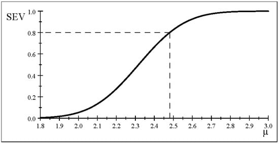
Figure 3. The post-data severity curve (accept $H_0)$.

The post-data severity evaluated for typical values reported in Table 4 reveals that the probability associated with the discrepancy relating to the estimate ${\overline{x}}_n=2.317$$({\gamma }_1=0.317)$ is never high enough to be the discrepancy warranted by ${\mathbf{x}}_0$ and test $T_{\alpha }$ since $SEV({\gamma }_1=0.317)=0.5$. This calls into question any claims relating to point estimates and observed CIs more generally since they represent an uncalibrated (it ignores the relevant uncertainty) single realization (${\mathbf{x}}_0$) of the sample $\mathbf{X}$ relating to the relevant sampling distribution.

Table 4. Post-data severity evaluation (SEV) for ${\mu }_1\le 2.0+\gamma$.

$\mathit{\gamma }$	0.05	0.1	0.15	0.20	0.30	0.317	0.40	0.481	0.60	0.70
${\mathit{\mu }}_{\mathbf{1}}$	2.05	2.1	2.15	2.2	2.3	2.317	2.4	2.481	2.6	2.7
$\mathsf{SEV}(\mu \le {\mu }_1)$	0.086	0.133	0.196	0.274	0.465	0.500	0.665	0.800	0.926	0.974

5.2. The Post-Data Severity and the Large n Problem

5.2.1. Case 1: Accept $H_0$

Empirical example 1 (continued). Consider scenario 2 where $[\left({\overline{x}}_n-{\mu }_0\right)/s_n]$ remains constant as n increases. Table 5 gives particular examples of n showing how ${\tau }_n\left({\mathbf{x}}_0\right)$ increases and ${\mu }_1$ decreases for a fixed $SEV\left(\gamma \right)=0.8$.

Table 5. Post-data severity $(SEV\left(\gamma \right)=0.8,{\mu }_1\le 2+{\gamma }_1,{\overline{x}}_n=2.317,s=1.941$).

n:	100	120	150	200	300	500	1000	2000	20,000	200,000
${\tau }_n\left({\mathbf{x}}_0\right)$:	1.633	1.789	2.0	2.310	2.829	3.652	5.165	7.304	23.097	73.038
${\mu }_1=2+\gamma$:	2.481	2.467	2.451	2.434	2.412	2.390	2.369	2.3535	2.329	2.321

Figure 4 presents the different SEV curves as n increases ($[\left({\overline{x}}_n-{\mu }_0\right)/s]$ held constant). It confirms the results of Table 5, by showing that the curves become steeper and steeper as n increases. This reduces the warranted discrepancy ${\gamma }_n^{‡}$ monotonically (Table 5), converging to the lower bound at ${\gamma }^{‡}\le 0.3217$$({\overline{x}}_n=2.317)$ as $n\to \infty .$ That is, the warranted discrepancies indicated on the x-axis, at a constant probability 0.8 (y-axis), become smaller and smaller as n increases, with the lower bound being the value of $\mu$ where its optimal estimator converges to ${\mu }^{*}$ with probability one as $n\to \infty$.

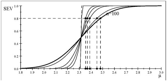
Figure 4. The severity curve (accept $H_0)$ for different n (same estimates).

This makes statistical sense in practice since ${\overline{X}}_n$ and $s_n$ are strongly consistent estimators of ${\mu }^{*}$ and ${\sigma }_{*},$ i.e., $\mathbb{P}({lim}_{n\to \infty }{\widehat{\theta }}_n\left(\mathbf{X}\right)={\theta }^{*})=1,$ and thus their accuracy (precision) improves as n increases beyond a certain threshold $n>N$. Recall that in the case of ‘accept $H_0$’ one is seeking the ‘smallest discrepancy’ from ${\mu }_0=2$. Hence, as n increases SEV renders the warranted discrepancy ${\gamma }_n^{‡}$ ‘more accurate’ by reducing it, until it reaches the lower bound around ${\gamma }^{‡}\le ({\overline{x}}_n-{\mu }_0)$ [${\mu }_1={\overline{x}}_n$] as $n\to \infty ;$ note that the latter is the most accurate value for ${\mu }^{*},$ only when ${\mathcal{M}}_{\mathit{\theta }}\left(\mathbf{x}\right)$ is statistically adequate!

5.2.2. Case 2: Reject $H_0$

Empirical example 3. Consider changing the estimate of $\mu$ to ${\overline{x}}_n=2.726$ retaining $s=1.941$, which yields:${\tau }_n\left({\mathbf{x}}_0\right)=3.740\left[0.00009\right],$ indicating ‘reject $H_0$’ in (4). In contrast to the case ‘accept $H_0$’, when the test ‘rejects $H_0$’ one is seeking the ‘largest’ discrepancy from ${\mu }_0=2$ with high probability. In light of ${\tau }_n\left({\mathbf{x}}_0\right)>0$, the relevant inferential claim is:$\mu \ge {\mu }_1={\mu }_0+\gamma ,$ for $\gamma >0,$ and its post-data probabilistic evaluation is based on:

$$\begin{array}{c}SEV(T_{\alpha };\mu \ge {\mu }_1)={\displaystyle \underset{\forall \mu \in {\mathrm{\Theta }}_1}{max}}\mathbb{P}(\tau \left(\mathbf{X}\right)<\tau \left({\mathbf{x}}_0\right);\mu ={\mu }_1)>p_1,\end{array}$$

(16)

where ${\mathrm{\Theta }}_1:=(2,\infty ),$ $p_1>0.5,$ and the evaluation of (16) is based on (15).

Table 6 indicates that the discrepancy $\gamma$ warranted with $SEV(T_{\alpha };\mu \ge {\mu }_1)=0.8$ is ${\gamma }^{‡}\le 0.562$ (${\mu }_1\le 2.562$), and the discrepancy for ${\mu }_1\le 2.726$ has $SEV(T_{\alpha };\mu \ge {\mu }_1)=0.5$.

Table 6. Post-data severity evaluation (SEV) for ${\mu }_1\ge 2+\gamma$.

$\mathit{\gamma }$	0.1	0.2	0.3	0.4	0.5	0.562	0.6	0.726	0.8	0.9
${\mathit{\mu }}_1$	2.1	2.2	2.3	2.4	2.5	2.562	2.6	2.562	2.6	2.7
$\mathsf{SEV}(\mu \ge {\mu }_1)$	0.999	0.996	0.984	0.951	0.876	0.800	0.741	0.500	0.352	0.186

Figure 5 depicts the severity curves for $n=100,200,500,1000,10,000$, indicating that keeping the probability constant at 0.8 (y-axis), as n increases (keeping $[\left({\overline{x}}_n-{\mu }_0\right)/s_n]$ constant) renders the curves steeper and steeper, thus ‘increasing’ the warranted discrepancy monotonically (x-axis) toward approaching the upper bound, which is the value of $\mu$ where its optimal estimator converges to ${\mu }^{*}$ with probability one as $n\to \infty .$ This is analogous to the case of ‘accept $H_0$’, with the lower bound replaced by an upper bound, which is equal to ${\mu }^{*}$ in both cases. That is, the SEV evaluation increases the precision of the discrepancy warranted with high (but constant) probability as n increases.

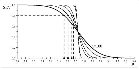
Figure 5. The severity curve (reject $H_0)$ for different n (same estimates).

Example 2A (Abouk et al., 2022) continued. The reported t-test result is:

$$\begin{array}{c}\frac{\sqrt{n}({\widehat{\beta }}_k-0)}{s\sqrt{q_{kk}}}=\frac{\sqrt{24,730,930}\left(0.004\right)}{\sqrt{98.932}}=2.0\left[0.045\right].\end{array}$$

What is the warranted discrepancy ${\gamma }^{†}$ from ${\beta }_k=0$ with high enough severity, say $0.977$ (in light of $n=24,730,930)?$ The answer is ${\beta }_k={\gamma }^{†}\le 0.0000001,$ which calls into question ${\widehat{\beta }}_k=0.004$, as well as Cohen’s $d\left({\mathbf{z}}_0\right)=0.0004$; see Ellis [29]. This confirms the tiny discrepancies from zero due to the large n problem conjectured in Section 4.1.

One might object to the above conclusion relating to the issue of spurious significance by countering that a tiny discrepancy is still different from zero, and thus, the statistical significance is well-grounded. Regrettably, such a counter-argument is based on a serious misconstrual of statistical inference in general, where learning from data takes the form of ‘statistical approximations’ framed in terms of a statistic or a pivot and its sampling distribution. This distinguishes statistics from other sub-fields of applied mathematics. No statistical inference is evaluated in terms of a binary choice of right and wrong! Indeed, this confusion lies at the heart of misinterpreting the binary accept/reject results as evidence for or against hypotheses or claims; see Mayo and Spanos [28].

Example 2B (Abouk et al. [33]) continued. As argued in Section 4.1, the reported results for the difference between two means exemplify the effect of the large n problem on the p-value. To be able to quantify that effect, however, one needs the exact p-values, but only two of the 42 reported p-values are given exactly, 0.8867 and 0.0056; the other 40 are reported as less than $0.0000$. Also, the particular sample sizes for the different reported tests are not given, and thus the overall $n_1$ and $n_1$ will be used. Focusing on the one with the p-value = 0.0056, one can retrieve the observed t-statistic, which can then be used for the SEV evaluation. For ${\overline{x}}_n=2.51$, ${\overline{y}}_n=2.51$, the observed t-statistic is $\tau \left({\mathbf{z}}_0\right)=2.77$, and using the SEV evaluation one can show that the warranted discrepancy $\gamma$ from $({\mu }_1-{\mu }_2)=0$ with SEV = $0.97$ ($N=6,108,194$) is ${\gamma }^{†}\le 0.00000068,$ which confirms that the t-test detects tiny discrepancies between the two estimated means, as conjectured in Section 4.1. That is, all but one (p-value = 0.8867) of the reported 42 test results in Table 2 (Abouk et al. [33] p. 43) constitute cases of spurious rejection of the null due to the large n problem. Even if one were to reduce N by a factor of 40, the warranted discrepancies would still be tiny.

5.2.3. Key Features of the Post-Data SEV Evaluation

(a)

The $SEV({\mu }_0+\gamma )$ is a post-data error probability, evaluated using hypothetical reasoning, that takes fully into account the testing statistical context in (11) and is guided by the sign and magnitude of ${\tau }_n\left({\mathbf{x}}_0\right)$ as indicators of the direction of the relevant discrepancies $\gamma$ from $\mu ={\mu }_0.$ This is particularly important because the factual reasoning, what if ${\theta =\theta }^{*}$, underlying point estimation and Confidence Intervals (CIs), does not apply post-data.

(b)

The $SEV({\mu }_0+\gamma )$ evaluation differs from other attempts to deal with the large n problem in so far as its outputting of the discrepancy ${\gamma }_1={\mu }_1-{\mu }_0$ is always based on the non-central distribution (Kraemer and Paik, [39]):

$$\begin{array}{c}(\frac{\sqrt{n}\left({\overline{X}}_n-{\mu }_0\right)}{s}-\frac{\sqrt{n}\left({\mu }_1-{\mu }_0\right)}{s})\stackrel{\mu ={\mu }_1}{\approx }\mathrm{St}(n-1),\mathrm{for}\mathrm{all}{\mu }_1\in {\mathrm{\Theta }}_1.\end{array}$$

(17)

This ensures that the warranted discrepancy ${\gamma }^{‡}$ is evaluated using the ‘same’ sample size n, counter-balancing the effect of n on ${\tau }_n\left({\mathbf{x}}_0\right).$ Note that ‘≈’ denotes an approximation.

(c)

The evaluation of the warranted ${\gamma }_n^{‡}$ with high probability accounts for the increase in n by enhancing its precision. As n increases ${\gamma }^{‡}$ will approach the value ${\widehat{\theta }}_n\left({\mathbf{x}}_0\right),$ since for a statistically adequate ${\mathcal{M}}_{\mathit{\theta }}\left(\mathbf{x}\right),$${\widehat{\theta }}_n\left({\mathbf{x}}_0\right)$ approaches ${\theta }^{*}$ due to its strong consistency.

(d)

The SEV can be used to address other foundational problems, including distinguishing between ‘statistical’ and ‘substantive’ significance. It also provides a testing-based effect size for the magnitude of the ‘scientific’ effect by addressing the problem with estimation-based effect sizes raised in Section 4.3. Also, the SEV evaluation can shed light on several proposed alternatives to (or modifications of) N-P testing by the replication crisis literature (Wasserstein et al. [40]), including replacing the p-value with effect sizes and observed CIs and redefining statistical significance (Benjamin et al. [41]) irrespective of the sample size n; see Spanos [25,37].

6. Summary and Conclusions

The large n problem arises naturally in the context of N-P testing due to the in-built trade-off between the type I and II error probabilities, around which the optimality of N-P tests revolves. This renders the accept/reject $H_0$ results and the p-value highly vulnerable to the large n problem. Hence, for $n>10,000$, the detection of statistical significance based on conventional significance levels will often be spurious since a consistent N-P test will detect smaller and smaller discrepancies as n increases; see Spanos [9].

The post-data severity (SEV) evaluation can address the large n problem by converting the unduly data-specific accept/reject $H_0$ ‘results’ into ‘evidence’ for a particular inferential claim of the form $\mathit{\theta }\gtrless {\mathit{\theta }}_0+{\gamma }_1,{\gamma }_1\ne 0$. This is framed in the form of the discrepancy ${\gamma }_1^{‡}$ warranted by data ${\mathbf{x}}_0$ and test $T_{\alpha }$ with high enough probability. The SEV evidential account is couched in terms of a post-data error probability that accounts for the uncertainty arising from the undue data-specificity of accept/reject $H_0$ results. The SEV differs from other attempts to address the large n problem in so far as its evaluation is invariably based on a non-central distribution whose non-centrality parameter uses the same n as the observed test statistic $\tau \left({\mathbf{x}}_0\right)$ to counter-balance the effect induced by n in outputting ${\gamma }_1.$

The SEV evaluation was illustrated above using two empirical results from Abouk et al. [33]. Example 2A concerns an estimated coefficient, ${\widehat{\beta }}_k=0.004$, SE$\left({\widehat{\beta }}_k\right)=0.002$, in a LR model, which is declared statistically significant at $\alpha =0.05$ with $n=24,730,930$. The SEV evaluation yields a discrepancy ${\gamma }^{†}\le 0.0000001$ from ${\beta }_k=0$ warranted by data ${\mathbf{z}}_0$ and the t-test with probability $0.977.$ Example 2B concerns the difference between two means whose estimates are ${\overline{x}}_{n_1}=2.51$, ${\overline{y}}_{n_2}=2.51$, but the t-test outputted $\tau \left({\mathbf{z}}_0\right)=2.77$ with $N=6,108,194$. The SEV evaluation yields a discrepancy ${\gamma }^{†}\le 0.00000068$ from $({\mu }_1-{\mu }_2)=0$ warranted by data ${\mathbf{z}}_0$ and the t-test with probability $0.97$. Both empirical examples represent cases of spurious statistical significance results stemming from exceptionally large sample sizes, $n=24,730,930,$ and $N=6,108,194$, respectively.

References

- Berkson, J. Some difficulties of interpretation encountered in the application of the chi-square test. J. Am. Stat. 1938, 33, 526–536. [Google Scholar] [CrossRef]
- Fisher, R.A. The Design of Experiments; Oliver and Boyd: Edinburgh, UK, 1935. [Google Scholar]
- Berkson, J. Tests of significance considered as evidence. J. Am. Assoc. 1942, 37, 325–335. [Google Scholar] [CrossRef]
- Fisher, R.A. Statistical Methods for Research Workers; Oliver and Boyd: Edinburgh, UK, 1925. [Google Scholar]
- Fisher, R.A. Note on Dr. Berkson’s criticism of tests of significance. J. Am. Stat. Assoc. 1943, 38, 103–104. [Google Scholar] [CrossRef][Green Version]
- Berkson, J. Experience with Tests of Significance: A Reply to Professor R. A. Fisher. J. Am. Assoc. 1943, 38, 242–246. [Google Scholar] [CrossRef]
- Spanos, A. Mis-Specification Testing in Retrospect. J. Econ. Surv. 2018, 32, 541–577. [Google Scholar] [CrossRef]
- Lindley, D.V. A statistical paradox. Biometrika 1957, 44, 187–192. [Google Scholar] [CrossRef]
- Spanos, A. Who Should Be Afraid of the Jeffreys-Lindley Paradox? Philos. Sci. 2013, 80, 73–93. [Google Scholar] [CrossRef]
- Lehmann, E.L. Significance level and power. Ann. Math. Stat. 1958, 29, 1167–1176. [Google Scholar] [CrossRef]
- Cohen, J. The statistical power of abnormal-social psychological research: A review. J. Abnorm. Soc. Psychol. 1962, 65, 145–153. [Google Scholar] [CrossRef]
- Freiman, J.A.; Chalmers, T.C.; Smith, H.; Kuebler, R.R. The importance of beta, the type II error and sample size in the design and interpretation of the randomized control trial. N. Engl. J. Med. 1978, 299, 690–694. [Google Scholar] [CrossRef]
- Lehmann, E.L. Testing Statistical Hypotheses, 2nd ed.; Wiley: New York, NY, USA, 1986. [Google Scholar]
- Cohen, J. Statistical Power Analysis for the Behavioral Sciences, 2nd ed.; Lawrence Erlbaum: Hoboken, NJ, USA, 1988. [Google Scholar]
- Good, I.J. Standardized tail-area probabilities. J. Stat. Comput. Simul. 1982, 16, 65–66. [Google Scholar] [CrossRef]
- Spanos, A. Where Do Statistical Models Come From? Revisiting the Problem of Specification. In Optimality: The Second Erich L. Lehmann Symposium; Rojo, J., Ed.; Lecture Notes-Monograph Series; Institute of Mathematical Statistics: Beachwood, OH, USA, 2006; Volume 49, pp. 98–119. [Google Scholar]
- Spanos, A. Introduction to Probability Theory and Statistical Inference: Empirical Modeling with Observational Data, 2nd ed.; Cambridge University Press: Cambridge, UK, 2019. [Google Scholar]
- Spanos, A. Statistical Misspecification and the Reliability of Inference: The simple t-test in the presence of Markov dependence. Korean Econ. Rev. 2009, 25, 165–213. [Google Scholar]
- Fisher, R.A. On the mathematical foundations of theoretical statistics. Philos. Trans. R. Soc. 1922, 222, 309–368. [Google Scholar]
- McCullagh, P. What is a statistical model? Ann. Stat. 2002, 30, 1225–1267. [Google Scholar] [CrossRef]
- Spanos, A. Statistical Adequacy and the Trustworthiness of Empirical Evidence: Statistical vs. Substantive Information. Econ. Model. 2010, 27, 1436–1452. [Google Scholar] [CrossRef]
- Rao, C.R. Statistics: Reflections on the Past and Visions for the Future. Amstat. News 2004, 327, 2–3. [Google Scholar]
- Spanos, A. Frequentist Model-based Statistical Induction and the Replication crisis. J. Quant. Econ. 2022, 20, 133–159. [Google Scholar] [CrossRef]
- Neyman, J.; Pearson, E.S. On the problem of the most efficient tests of statistical hypotheses. Philos. Trans. R. Soc. 1933, 231, 289–337. [Google Scholar]
- Spanos, A. How the Post-data Severity Converts Testing Results into Evidence for or Against Pertinent Inferential Claims. Entropy 2023. under review. [Google Scholar]
- Spanos, A. Severity and Trustworthy Evidence: Foundational Problems versus Misuses of Frequentist Testing. Philos. Sci. 2022, 89, 378–397. [Google Scholar] [CrossRef]
- Mayo, G.D.; Spanos, A. Severe Testing as a Basic Concept in a Neyman-Pearson Philosophy of Induction. Br. J. Philos. Sci. 2006, 57, 323–357. [Google Scholar] [CrossRef]
- Mayo, D.G.; Spanos, A. Error Statistics. In The Handbook of Philosophy of Science; Gabbay, D., Thagard, P., Woods, J., Eds.; Elsevier: Amsterdam, The Netherlands, 2011; Volume 7: Philosophy of Statistics, pp. 151–196. [Google Scholar]
- Ellis, P.D. The Essential Guide to Effect Sizes: Statistical Power, Meta-Analysis, and the Interpretation of Research Results; Cambirdge University Press: Cambridge, UK, 2010. [Google Scholar]
- Fisher, R.A. Statistical methods and scientific induction. J. R. Soc. Ser. Stat. Methodol. 1955, 17, 69–78. [Google Scholar] [CrossRef]
- Fisher, R.A. Two new properties of mathematical likelihood. Proc. R. Soc. Lond. Ser. 1934, 144, 285–307. [Google Scholar]
- Pesko, M.F.; Warman, C. Re-exploring the early relationship between teenage cigarette and e-cigarette use using price and tax changes. Health Econ. 2022, 31, 137–153. [Google Scholar] [CrossRef] [PubMed]
- Abouk, R.; Adams, S.; Feng, B.; Maclean, J.C.; Pesko, M. The Effects of e-cigarette taxes on pre-pregnancy and prenatal smoking. NBER Work. Pap. 2022, 26126, Revised June 2022. Available online: https://www.nber.org/system/files/workingpapers/w26126/w26126.pdf (accessed on 5 October 2023).
- Thompson, B. Foundations of Behavioral Statistics: An Insight-Based Approach; Guilford Press: New York, NY, USA, 2006. [Google Scholar]
- Abelson, R.P. Statistics as Principled Argument; Lawrence Erlbaum: Hoboken, NJ, USA, 1995. [Google Scholar]
- Spanos, A. Bernoulli’s golden theorem in retrospect: Error probabilities and trustworthy evidence. Synthese 2021, 199, 13949–13976. [Google Scholar] [CrossRef]
- Spanos, A. Revisiting noncentrality-based confidence intervals, error probabilities and estimation-based effect sizes. J. Math. 2021, 104, 102580. [Google Scholar] [CrossRef]
- Owen, D.B. Survey of Properties and Applications of the Noncentral t-Distribution. Technometrics 1968, 10, 445–478. [Google Scholar] [CrossRef]
- Kraemer, H.C.; Paik, M. A central t approximation to the noncentral t distribution. Technometrics 1979, 21, 357–360. [Google Scholar] [CrossRef]
- Wasserstein, R.L.; Schirm, A.L.; Lazar, N.A. Moving to a world beyond “p < 0.05”. Am. Stat. 2019, 73, 1–19. [Google Scholar]
- Benjamin, D.J.; Berger, J.O.; Johannesson, M.; Nosek, B.A.; Wagenmakers, E.J.; Berk, R.; Bollen, K.A.; Brembs, B.; Brown, L.; Camerer, C.; et al. Redefine statistical significance. Nat. Hum. Behav. 2017, 33, 6–10. [Google Scholar] [CrossRef]
Disclaimer/Publisher’s Note: The statements, opinions and data contained in all publications are solely those of the individual author(s) and contributor(s) and not of MDPI and/or the editor(s). MDPI and/or the editor(s) disclaim responsibility for any injury to people or property resulting from any ideas, methods, instructions or products referred to in the content. |
© 2023 by the author. Licensee MDPI, Basel, Switzerland. This article is an open access article distributed under the terms and conditions of the Creative Commons Attribution (CC BY) license (https://creativecommons.org/licenses/by/4.0/).