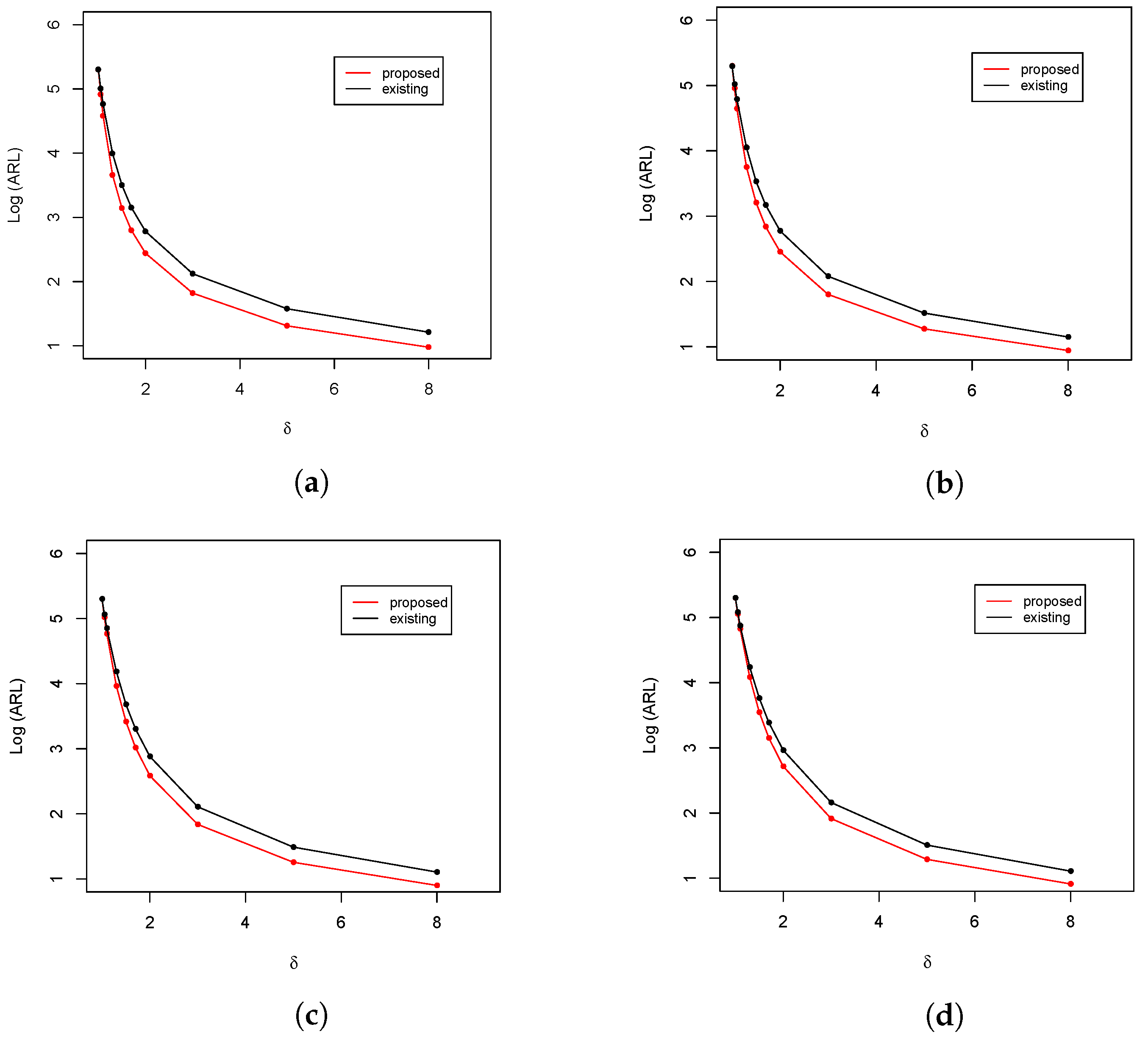
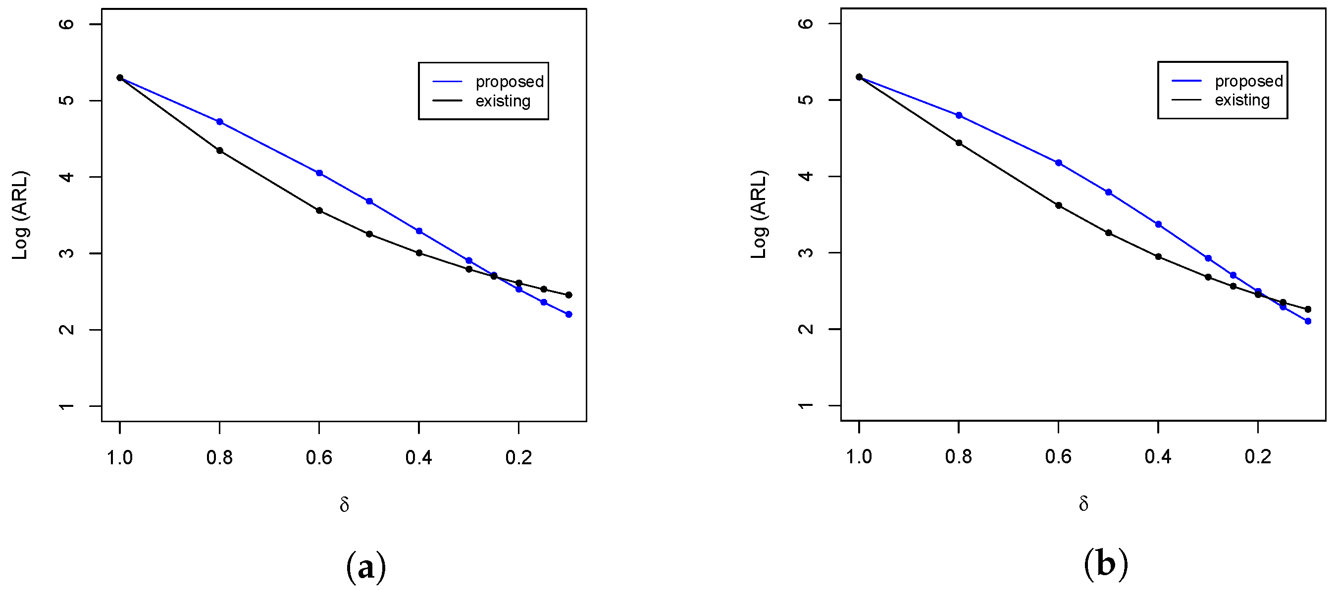
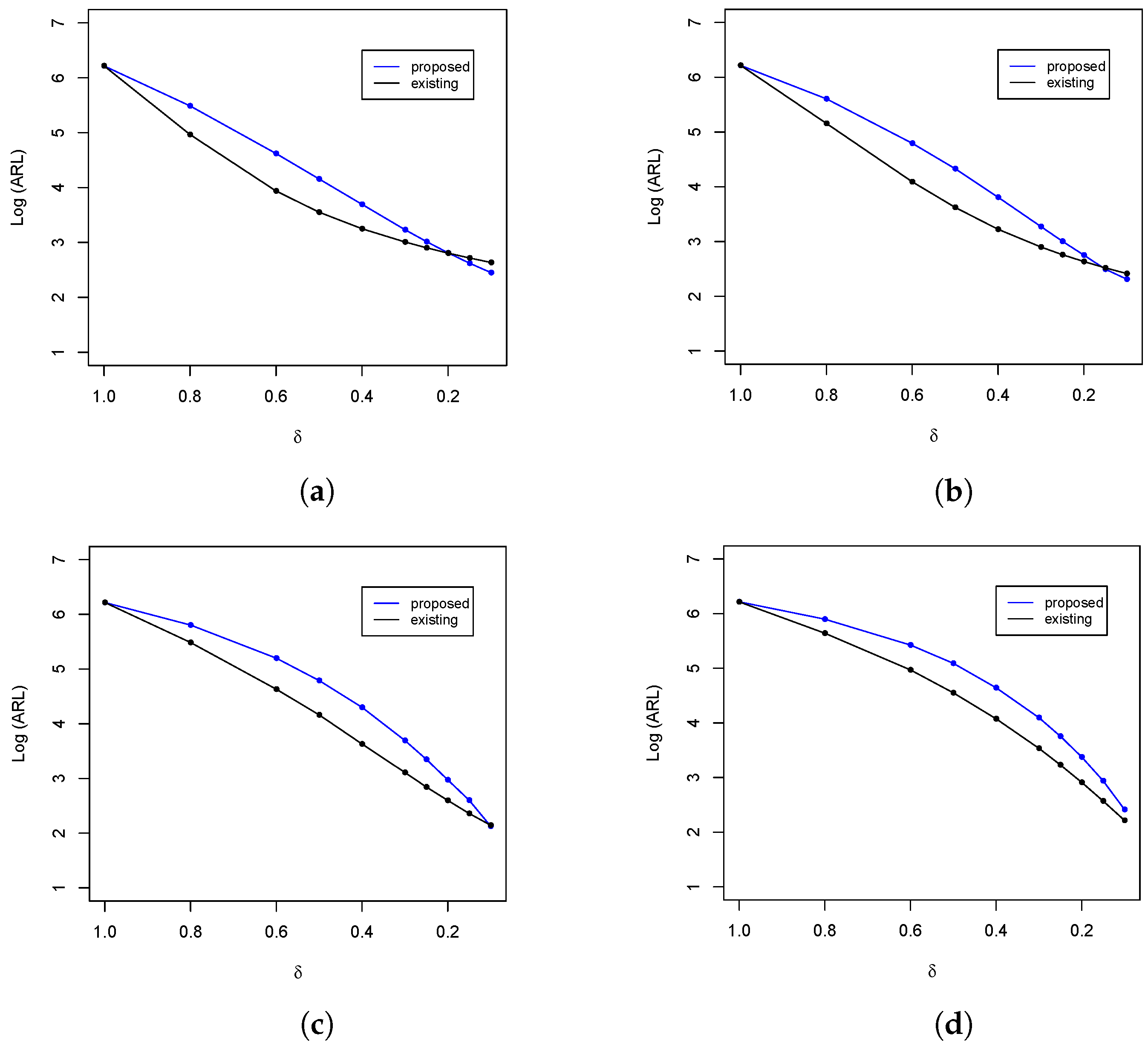
Figure 1.
ARL comparison of the upper-sided control charts at and . (a) ; (b) ; (c) ; and (d) .
Figure 1.
ARL comparison of the upper-sided control charts at and . (a) ; (b) ; (c) ; and (d) .
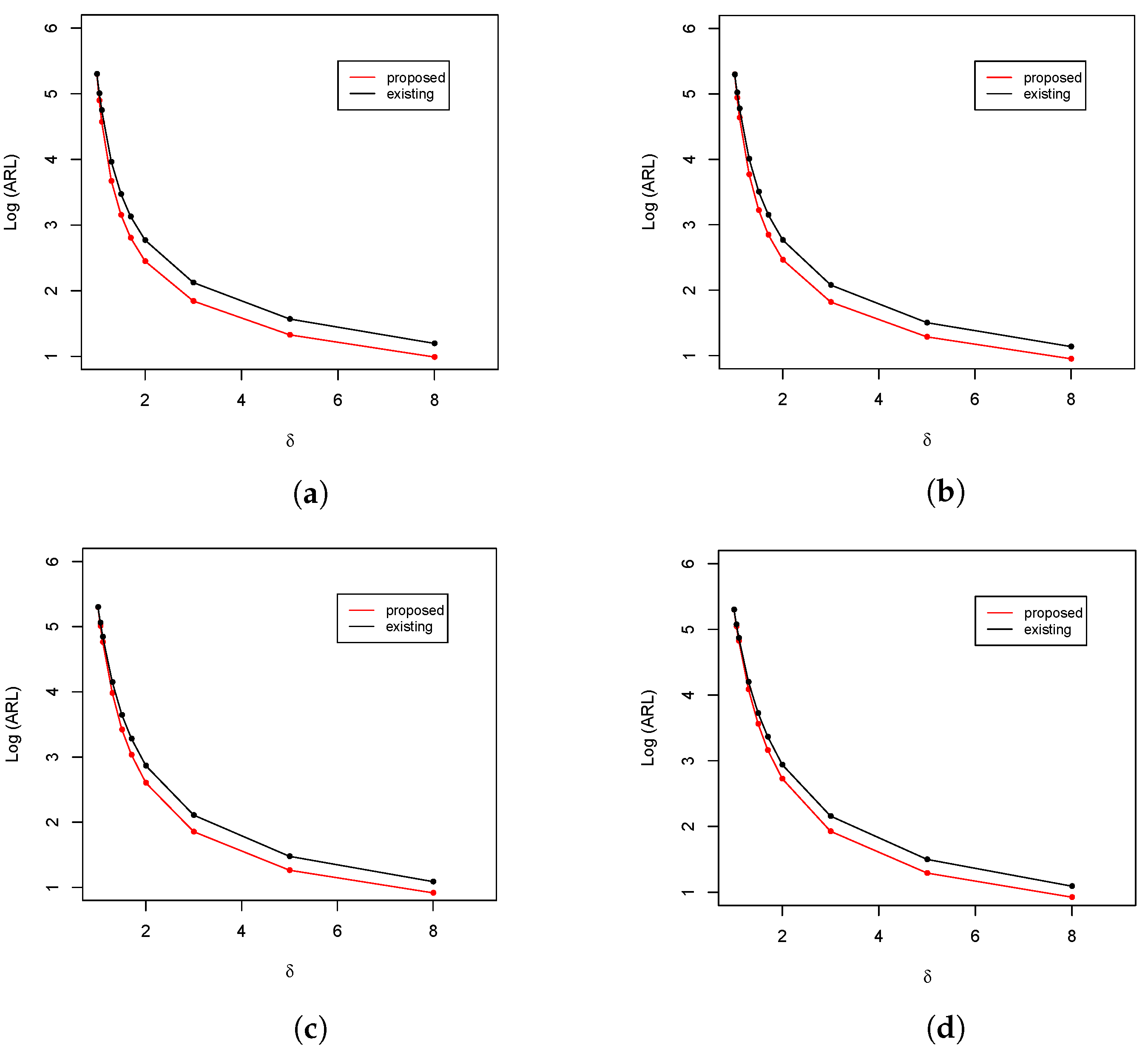
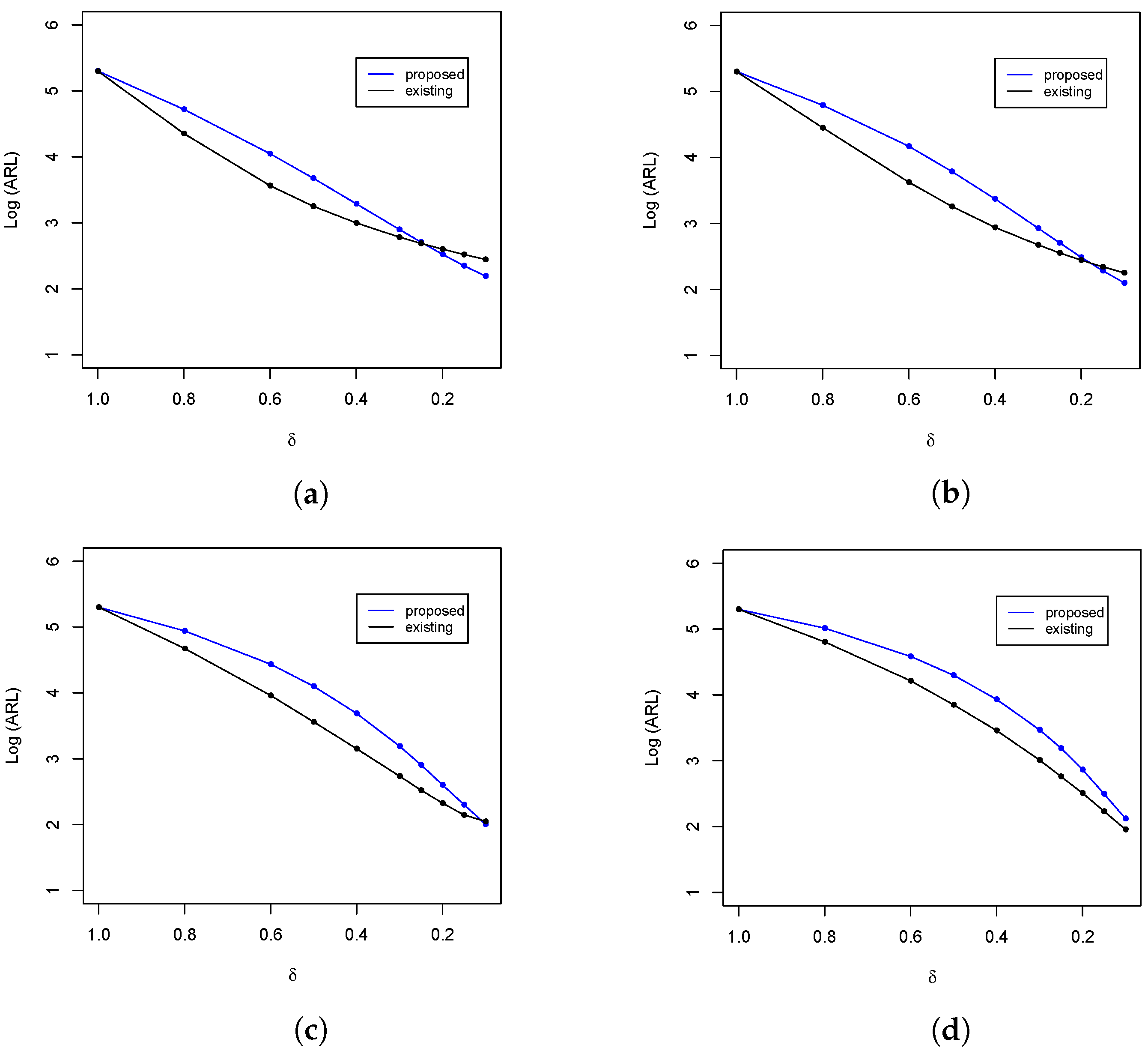
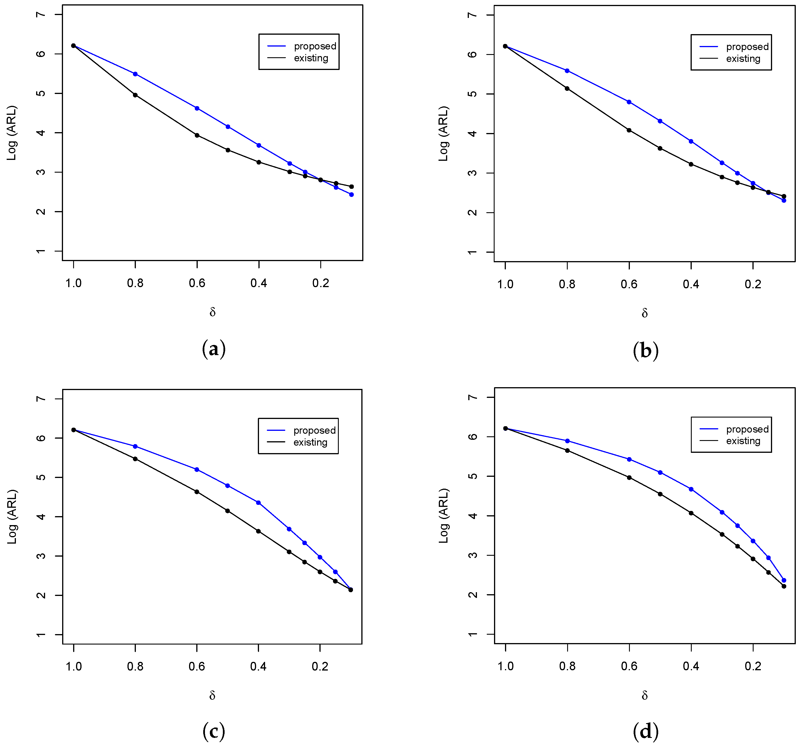
Figure 2.
ARL comparison of the upper-sided control charts at with . (a) ; (b) ; (c) ; and (d) .
Figure 2.
ARL comparison of the upper-sided control charts at with . (a) ; (b) ; (c) ; and (d) .
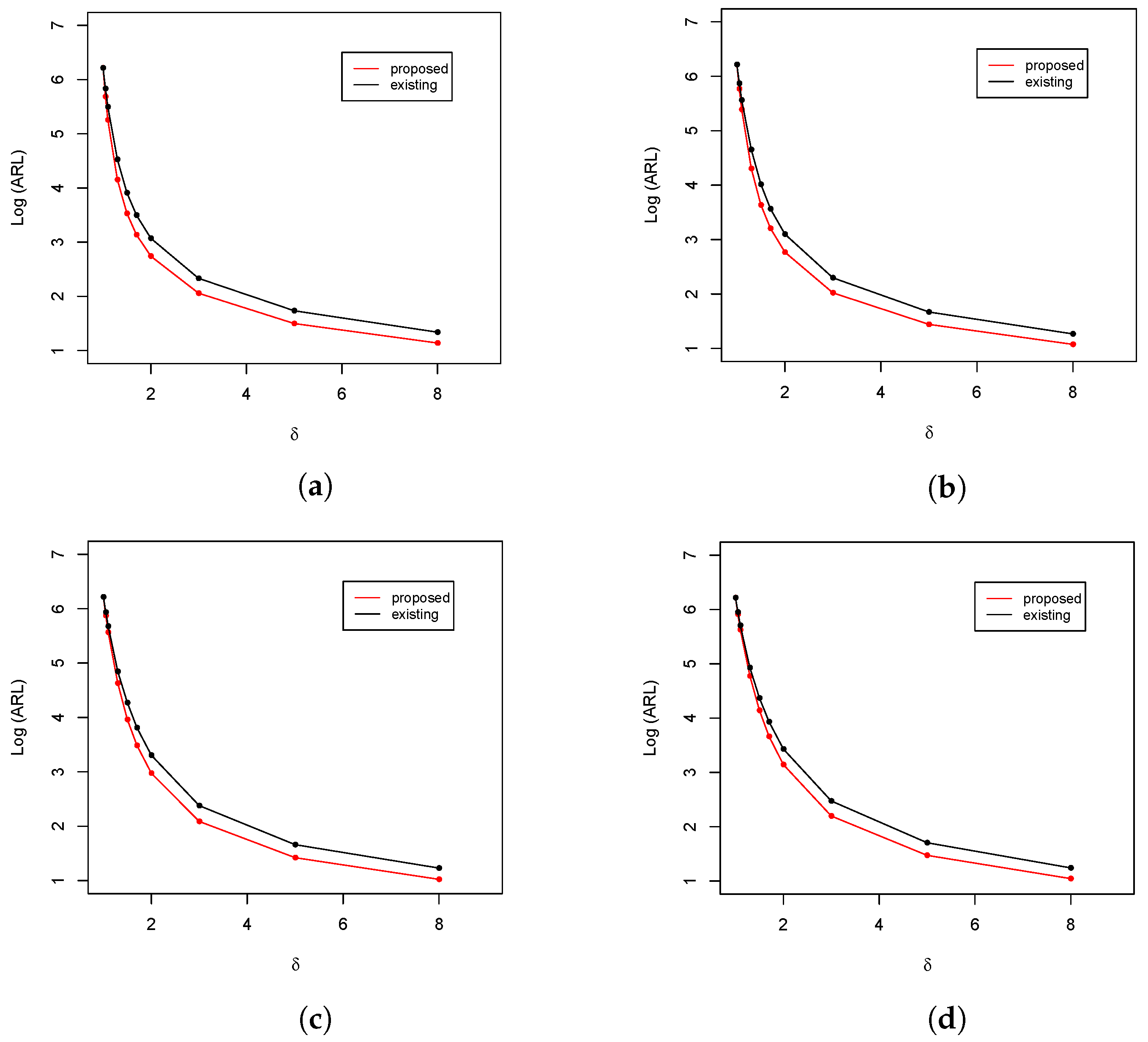
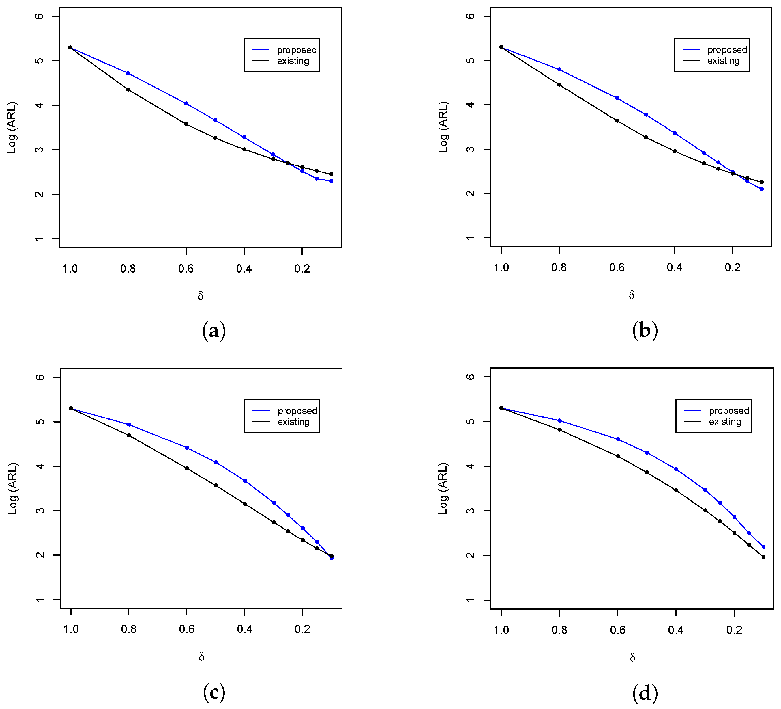
Figure 3.
ARL comparison of the upper-sided control charts at and . (a) ; (b) ; (c) ; and (d) .
Figure 3.
ARL comparison of the upper-sided control charts at and . (a) ; (b) ; (c) ; and (d) .
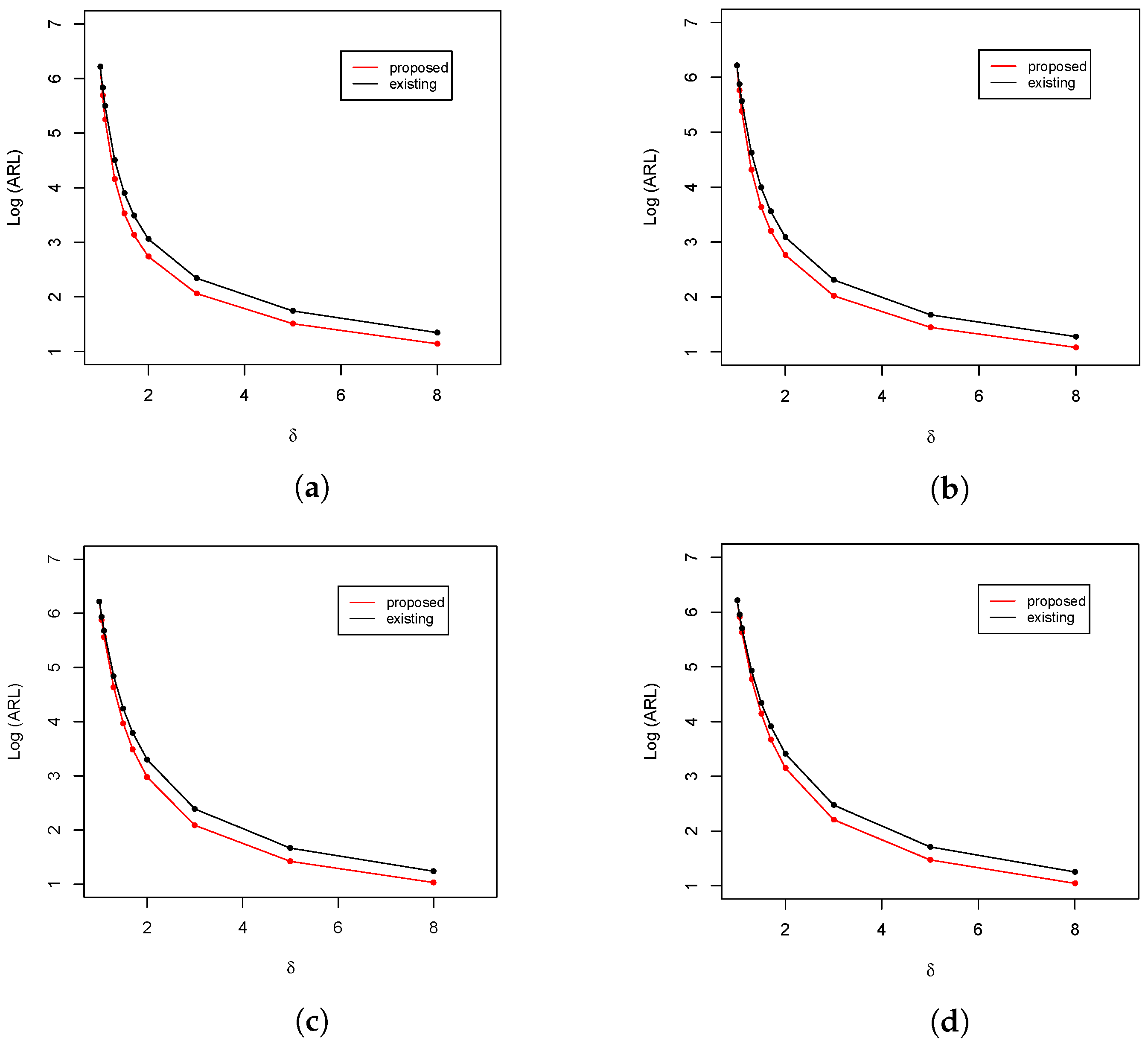
Figure 4.
ARL comparison of the upper-sided control charts at and . (a) ; (b) ; (c) ; and (d) .
Figure 4.
ARL comparison of the upper-sided control charts at and . (a) ; (b) ; (c) ; and (d) .
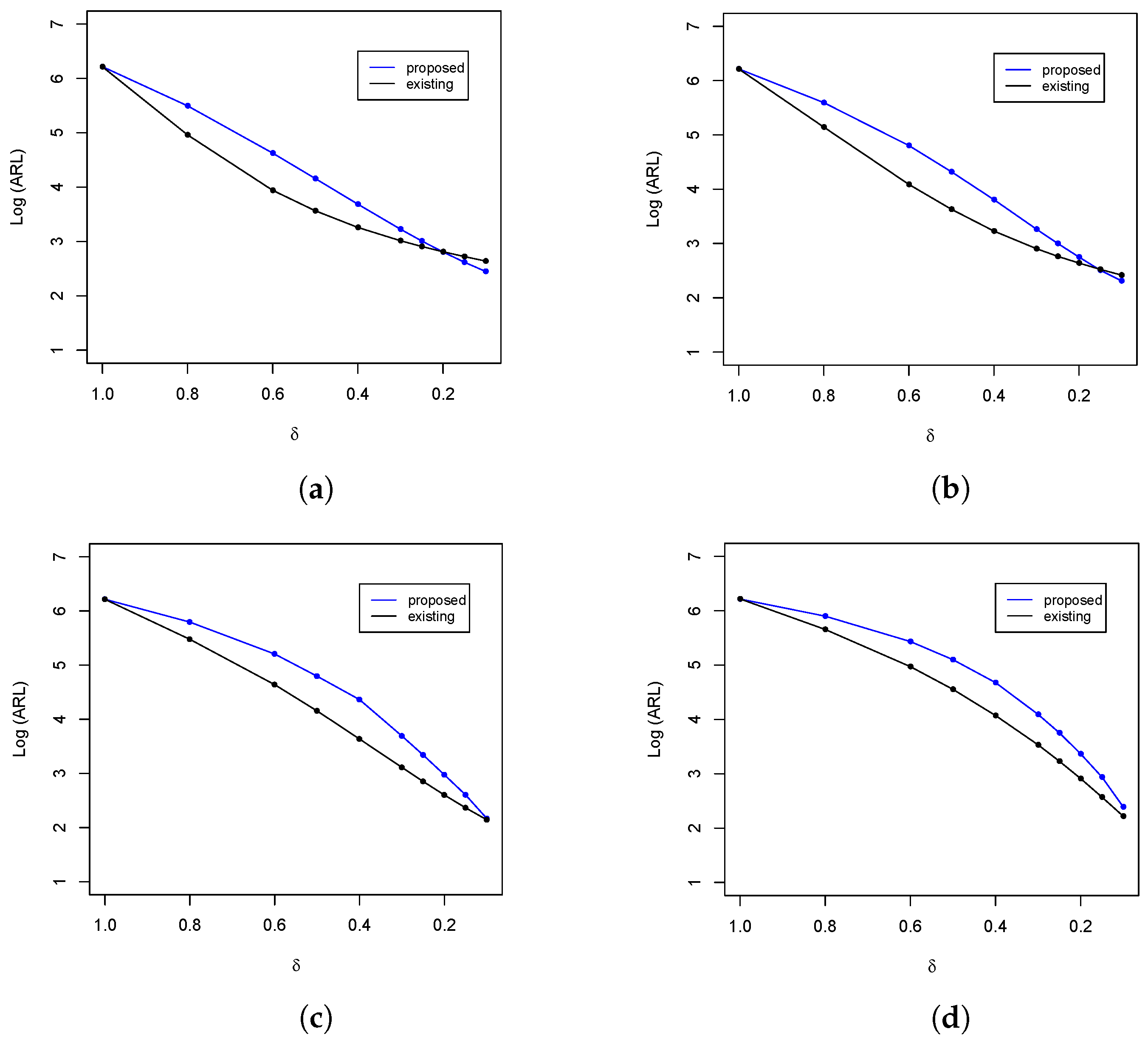
Figure 5.
ARL comparison of the upper-sided control charts at and . (a) ; (b) ; (c) ; and (d) .
Figure 5.
ARL comparison of the upper-sided control charts at and . (a) ; (b) ; (c) ; and (d) .
Figure 6.
ARL comparison of the upper-sided control charts at and . (a) ; (b) ; (c) ; and (d) .
Figure 6.
ARL comparison of the upper-sided control charts at and . (a) ; (b) ; (c) ; and (d) .
Figure 7.
ARL comparison of the lower-sided control charts at with . (a) ; (b) ; (c) ; and (d) .
Figure 7.
ARL comparison of the lower-sided control charts at with . (a) ; (b) ; (c) ; and (d) .
Figure 8.
ARL comparison of the lower-sided control charts at and . (a) ; (b) ; (c) ; and (d) .
Figure 8.
ARL comparison of the lower-sided control charts at and . (a) ; (b) ; (c) ; and (d) .
Figure 9.
ARL comparison of the lower-sided control charts at and . (a) ; (b) ; (c) ; and (d) .
Figure 9.
ARL comparison of the lower-sided control charts at and . (a) ; (b) ; (c) ; and (d) .
Figure 10.
ARL comparison of the lower-sided control charts at with . (a) ; (b) ; (c) ; and (d) .
Figure 10.
ARL comparison of the lower-sided control charts at with . (a) ; (b) ; (c) ; and (d) .
Figure 11.
ARL comparison of the lower-sided control charts at and . (a) ; (b) ; (c) ; and (d) .
Figure 11.
ARL comparison of the lower-sided control charts at and . (a) ; (b) ; (c) ; and (d) .
Figure 12.
ARL comparison of the lower-sided control charts at and . (a) ; (b) ; (c) ; and (d) .
Figure 12.
ARL comparison of the lower-sided control charts at and . (a) ; (b) ; (c) ; and (d) .
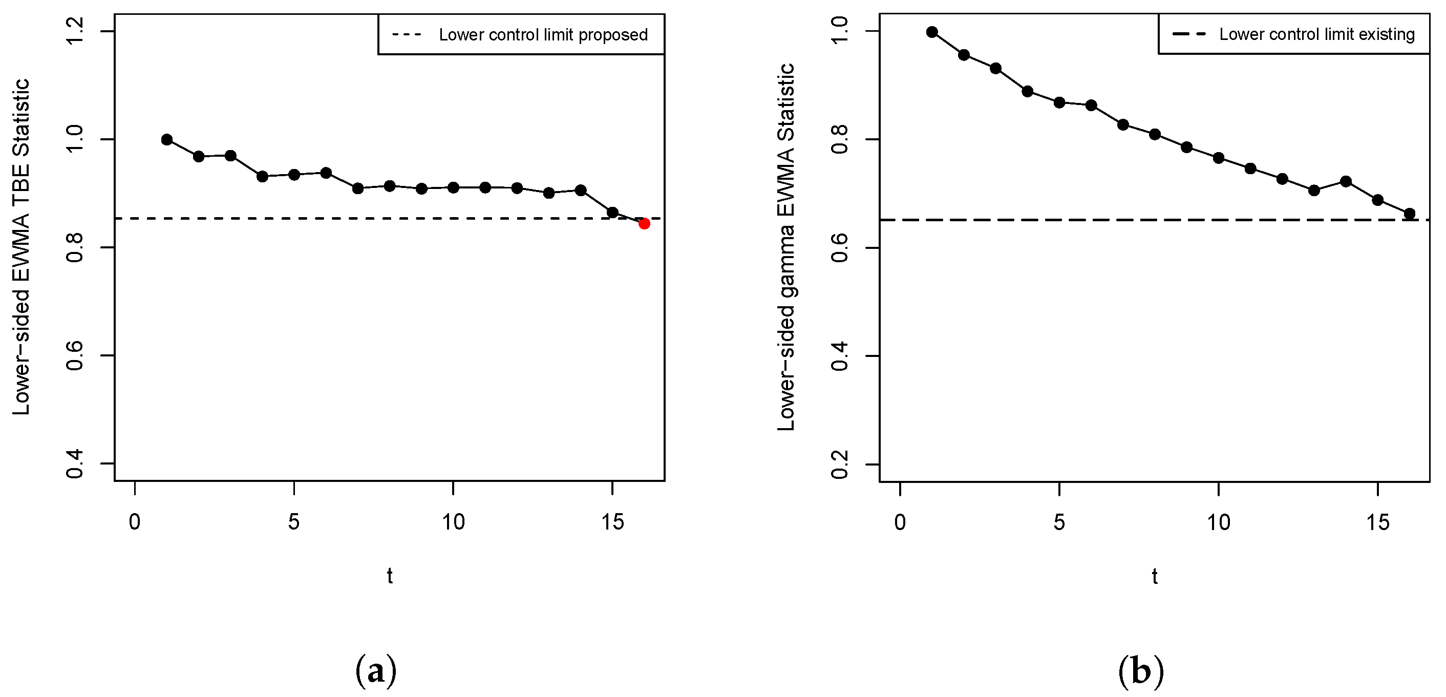
Figure 13.
Lower-sided proposed and existing TBE EWMA charts. (a) Proposed chart; (b) existing chart.
Figure 13.
Lower-sided proposed and existing TBE EWMA charts. (a) Proposed chart; (b) existing chart.
Table 1.
The UCL of the upper-sided TBE EWMA and existing gamma EWMA charts with , and .
Table 1.
The UCL of the upper-sided TBE EWMA and existing gamma EWMA charts with , and .
| Proposed |
|---|
| | () |
| n | 0.05 | 0.07 | 0.1 | 0.2 | 0.3 | 0.5 | 0.7 | 0.9 |
| 10 | 2.0933 | 2.1847 | 2.313 | 2.701 | 3.0671 | 3.791 | 4.5176 | 5.2624 |
| 30 | 2.0936 | 2.1849 | 2.3134 | 2.7026 | 3.0685 | 3.7937 | 4.5177 | 5.265 |
| 50 | 2.0941 | 2.1861 | 2.3147 | 2.7047 | 3.0715 | 3.798 | 4.5255 | 5.2715 |
| 100 | 2.0944 | 2.1862 | 2.3151 | 2.7044 | 3.0718 | 3.7973 | 4.5247 | 5.2718 |
| 200 | 2.0928 | 2.1848 | 2.3129 | 2.7016 | 3.0683 | 3.7914 | 4.5182 | 5.2644 |
| 300 | 2.0925 | 2.1845 | 2.3118 | 2.6996 | 3.0646 | 3.7851 | 4.5087 | 5.2552 |
| 350 | 2.0929 | 2.1837 | 2.3116 | 2.7005 | 3.0657 | 3.7854 | 4.5135 | 5.2549 |
| 2.0914 | 2.1848 | 2.3138 | 2.7059 | 3.0712 | 3.7887 | 4.5167 | 5.2622 |
| Existing |
| 10 | 0.7763 | 0.8597 | 0.977 | 1.3359 | 1.6734 | 2.3256 | 2.9743 | 3.6149 |
| 30 | 0.776 | 0.8599 | 0.9772 | 1.3356 | 1.6736 | 2.3256 | 2.9727 | 3.6151 |
| 50 | 0.7764 | 0.8601 | 0.9781 | 1.337 | 1.6753 | 2.3304 | 2.9779 | 3.6209 |
| 100 | 0.7769 | 0.861 | 0.9781 | 1.337 | 1.6756 | 2.3286 | 2.9739 | 3.6168 |
| 200 | 0.7764 | 0.8606 | 0.9787 | 1.3376 | 1.675 | 2.3251 | 2.9677 | 3.6078 |
| 300 | 0.7773 | 0.8624 | 0.9798 | 1.3396 | 1.6767 | 2.3285 | 2.9709 | 3.6126 |
| 350 | 0.7776 | 0.8622 | 0.9796 | 1.3391 | 1.6768 | 2.3288 | 2.9719 | 3.617 |
| 0.7779 | 0.8619 | 0.9811 | 1.3386 | 1.6766 | 2.3264 | 2.9654 | 3.6098 |
Table 2.
The UCL of the upper-sided TBE EWMA and existing upper-sided gamma EWMA charts with , and .
Table 2.
The UCL of the upper-sided TBE EWMA and existing upper-sided gamma EWMA charts with , and .
| Proposed |
|---|
| | () |
| n | 0.05 | 0.07 | 0.1 | 0.2 | 0.3 | 0.5 | 0.7 | 0.9 |
| 10 | 2.1542 | 2.2592 | 2.4043 | 2.8449 | 3.2624 | 4.0857 | 4.9226 | 5.7801 |
| 30 | 2.1547 | 2.2595 | 2.4049 | 2.846 | 3.2629 | 4.0862 | 4.9236 | 5.7819 |
| 50 | 2.1549 | 2.2598 | 2.4053 | 2.8468 | 3.2636 | 4.0878 | 4.9278 | 5.7841 |
| 100 | 2.1548 | 2.2595 | 2.4049 | 2.8468 | 3.262 | 4.0861 | 4.9273 | 5.7811 |
| 200 | 2.1541 | 2.2583 | 2.4032 | 2.8457 | 3.2603 | 4.0843 | 4.9263 | 5.779 |
| 300 | 2.1538 | 2.2576 | 2.4028 | 2.8449 | 3.2592 | 4.0833 | 4.9228 | 5.7765 |
| 350 | 2.1535 | 2.2575 | 2.4026 | 2.8448 | 3.259 | 4.0832 | 4.9222 | 5.7772 |
| 2.1531 | 2.2571 | 2.4021 | 2.8431 | 3.2596 | 4.0869 | 4.9208 | 5.7796 |
| Existing |
| 10 | 0.8249 | 0.9208 | 1.0551 | 1.4663 | 1.8552 | 2.6135 | 3.364 | 4.1178 |
| 30 | 0.8481 | 0.9207 | 1.055 | 1.4664 | 1.8551 | 2.6149 | 3.3649 | 4.1179 |
| 50 | 0.825 | 0.9213 | 1.0552 | 1.4674 | 1.8567 | 2.6167 | 3.3682 | 4.123 |
| 100 | 0.8253 | 0.9214 | 1.0554 | 1.4676 | 1.8566 | 2.6156 | 3.3666 | 4.1191 |
| 200 | 0.8257 | 0.9218 | 1.0564 | 1.4703 | 1.8602 | 2.618 | 3.3702 | 4.1204 |
| 300 | 0.8258 | 0.9227 | 1.0575 | 1.4701 | 1.8582 | 2.6161 | 3.3688 | 4.1183 |
| 350 | 0.8257 | 0.9221 | 1.0571 | 1.4704 | 1.8588 | 2.6162 | 3.3686 | 4.12 |
| 0.8256 | 0.9214 | 1.0566 | 1.4685 | 1.8563 | 2.6131 | 3.3675 | 4.1193 |
Table 3.
The UCL of the upper-sided TBE EWMA and existing upper-sided gamma EWMA charts with , and .
Table 3.
The UCL of the upper-sided TBE EWMA and existing upper-sided gamma EWMA charts with , and .
| Proposed |
|---|
| | () |
| n | 0.05 | 0.07 | 0.1 | 0.2 | 0.3 | 0.5 | 0.7 | 0.9 |
| 10 | 2.182 | 2.2927 | 2.4468 | 2.9127 | 3.3551 | 4.2298 | 5.1173 | 6.0301 |
| 30 | 2.1817 | 2.2924 | 2.4466 | 2.913 | 3.3553 | 4.2301 | 5.1168 | 6.0275 |
| 50 | 2.182 | 2.2926 | 2.4466 | 2.9129 | 3.3551 | 4.2306 | 5.1178 | 6.029 |
| 100 | 2.1821 | 2.2929 | 2.4462 | 2.9136 | 3.3558 | 4.2337 | 5.1204 | 6.0322 |
| 200 | 2.1816 | 2.292 | 2.4456 | 2.9129 | 3.355 | 4.2323 | 5.12 | 6.0356 |
| 300 | 2.1809 | 2.291 | 2.444 | 2.9089 | 3.3513 | 4.2281 | 5.1138 | 6.0274 |
| 350 | 2.1807 | 2.2911 | 2.4441 | 2.909 | 3.3512 | 4.2286 | 5.1158 | 6.0354 |
| 2.1814 | 2.2914 | 2.4442 | 2.9097 | 3.353 | 4.2285 | 5.1184 | 6.0333 |
| Existing |
| 10 | 0.848 | 0.9498 | 1.0917 | 1.5304 | 1.9451 | 2.7543 | 3.557 | 4.3608 |
| 30 | 0.8481 | 0.9501 | 1.092 | 1.5305 | 1.9451 | 2.7548 | 3.5585 | 4.3639 |
| 50 | 0.8483 | 0.9504 | 1.0927 | 1.5311 | 1.9468 | 2.7569 | 3.5604 | 4.3661 |
| 100 | 0.8487 | 0.9506 | 1.0928 | 1.5309 | 1.9453 | 2.7555 | 3.5587 | 4.3646 |
| 200 | 0.8483 | 0.9504 | 1.0928 | 1.5307 | 1.9448 | 2.7558 | 3.5602 | 4.3654 |
| 300 | 0.8489 | 0.9512 | 1.0939 | 1.5309 | 1.9458 | 2.7578 | 3.5603 | 4.369 |
| 350 | 0.8486 | 0.9507 | 1.0936 | 1.531 | 1.9464 | 2.7589 | 3.5613 | 4.3709 |
| 0.8488 | 0.9507 | 1.0932 | 1.5306 | 1.9455 | 2.7552 | 3.5625 | 4.3719 |
Table 4.
() profiles of the upper-sided EWMA TBE and upper-sided gamma EWMA chart when = 370.
Table 4.
() profiles of the upper-sided EWMA TBE and upper-sided gamma EWMA chart when = 370.
| | | () | 0.05 | 0.07 | 0.1 | 0.2 | 0.3 | 0.5 | 0.7 | 0.9 |
|---|
| | | |
2.1531
|
2.2571
|
2.4021
|
2.8431
|
3.2596
|
4.0869
|
4.9208
|
5.7796
|
|---|
|
Charts
| |
0.8256
|
0.9214
|
1.0566
|
1.4685
|
1.8563
|
2.6131
|
3.3675
|
4.1193
|
|---|
| 1 | Proposed | | 370.18 (365.38) | 370.3 (363.29) | 370.3 (365.05) | 370.52 (367.98) | 370.29 (363.96) | 370.21 (371.87) | 370.29 (374.89) | 370.29 (376.85) |
| | Existing | | 369.65 (369.58) | 369.65 (365.12) | 370.41 (363.49) | 370.17 (373.45) | 370.04 (374.61) | 370.33 (376.42) | 370.11 (373.59) | 369.93 (372.26) |
| 1.05 | Proposed | | 229.07 (223.64) | 237.1 (234.47) | 243.83 (240.24) | 257.33 (255.38) | 267.42 (264.37) | 279.11 (277.42) | 281.99 (283.12) | 285.28 (288.43) |
| | Existing | | 256.46 (245.83) | 259.41 (249.36) | 265.3 (255.38) | 277.03 (272.1) | 282.44 (282.58) | 288.46 (287.7) | 291.67 (291.34) | 292.21 (291.46) |
| 1.1 | Proposed | | 152.07 (144.54) | 159.51 (154.49) | 167.72 (165) | 185.87 (184.41) | 198.22 (199.29) | 215.35 (215.34) | 221.18 (220.76) | 225.9 (227.68) |
| | Existing | | 189.14 (181.44) | 193.28 (185.06) | 200.27 (193.18) | 213.05 (206.74) | 219.05 (213.91) | 227.51 (223.21) | 234.54 (233.02) | 236.22 (233.7) |
| 1.3 | Proposed | | 53.62 (45.77) | 56.75 (50.17) | 60.93 (55.5) | 72.36 (69.13) | 80.15 (79.25) | 93.15 (92.98) | 100.89 (101.45) | 105.74 (104.89) |
| | Existing | | 75.93 (67.89) | 78.82 (72.23) | 83.53 (77.75) | 93.64 (90.17) | 100.82 (97.52) | 108.73 (107.09) | 113.98 (112.92) | 116.93 (116.28) |
| 1.5 | Proposed | | 30.04 (23.57) | 30.99 (25.48) | 32.79 (28.13) | 38.18 (35.82) | 43.01 (41.15) | 50.52 (49.64) | 56.16 (55.43) | 60.15 (59.78) |
| | Existing | | 43.14 (35.94) | 44.49 (39.41) | 46.77 (43.21) | 52.62 (50.67) | 56.8 (55.39) | 62.37 (62.62) | 65.99 (65.53) | 69.19 (67.61) |
| 1.7 | Proposed | | 20.61 (15.31) | 20.99 (16.36) | 21.67 (17.67) | 24.83 (22.16) | 27.71 (25.69) | 32.71 (30.95) | 36.34 (35.35) | 39.26 (37.96) |
| | Existing | | 29.19 (23.04) | 29.72 (24.62) | 30.88 (26.88) | 34.63 (32.7) | 37.34 (36.33) | 41.64 (41.35) | 44.38 (44.46) | 46.13 (46.52) |
| 2 | Proposed | | 14.13 (9.88) | 14.11 (10.41) | 14.35 (11.19) | 15.74 (13.59) | 17.26 (15.77) | 20.02 (18.91) | 22.46 (21.49) | 24.18 (23.37) |
| | Existing | | 19.82 (14.76) | 19.84 (15.56) | 20.17 (16.82) | 22.08 (20.18) | 23.69 (22.6) | 26.23 (25.48) | 27.95 (27.46) | 28.98 (28.48) |
| 3 | Proposed | | 7.35 (4.87) | 7.17 (4.91) | 7.05 (5.05) | 7.13 (5.62) | 7.43 (6.21) | 8.25 (7.35) | 8.97 (8.27) | 9.59 (9.05) |
| | Existing | | 9.77 (6.82) | 9.53 (6.98) | 9.41 (7.22) | 9.57 (8.18) | 9.99 (8.96) | 10.72 (10.01) | 11.45 (10.85) | 11.9 (11.34) |
| 5 | Proposed | | 4.22 (2.68) | 4.1 (2.66) | 3.98 (2.68) | 3.85 (2.78) | 3.87 (2.96) | 4.03 (3.32) | 4.24 (3.63) | 4.45 (3.92) |
| | Existing | | 5.41 (3.68) | 5.21 (3.67) | 5.07 (3.72) | 4.92 (3.86) | 4.97 (4.1) | 5.2 (4.48) | 5.38 (4.83) | 5.53 (5.03) |
| 8 | Proposed | | 2.94 (1.85) | 2.87 (1.83) | 2.78 (1.81) | 2.67 (1.82) | 2.64 (1.85) | 2.66 (1.98) | 2.74 (2.12) | 2.82 (2.29) |
| | Existing | | 3.64 (2.47) | 3.51 (2.43) | 3.41 (2.4) | 3.27 (2.43) | 3.23 (2.5) | 3.28 (2.66) | 3.35 (2.78) | 3.42 (2.89) |
Table 5.
() profiles of the upper-sided TBE EWMA and upper-sided gamma EWMA chart when and = 370.
Table 5.
() profiles of the upper-sided TBE EWMA and upper-sided gamma EWMA chart when and = 370.
| | | () | 0.05 | 0.07 | 0.1 | 0.2 | 0.3 | 0.5 | 0.7 | 0.9 |
|---|
| | | |
2.1535
|
2.2575
|
2.4026
|
2.8448
|
3.259
|
4.0832
|
4.9222
|
5.7772
|
|---|
|
Charts
| |
0.8257
|
0.9221
|
1.0571
|
1.4704
|
1.8588
|
2.6162
|
3.3686
|
4.12
|
|---|
| 1 | Proposed | | 369.51 (367.59) | 369.58 (366.37) | 370.02 (370.38) | 369.76 (367.64) | 369.76 (365.71) | 369.81 (371.88) | 370.06 (372.16) | 370.04 (374.83) |
| | Existing | | 369.94 (364.82) | 369.64 (363.21) | 370.1 (363.25) | 370.23 (370.63) | 369.99 (371.85) | 370.04 (375.54) | 369.91 (374.79) | 370.49 (373.28) |
| 1.05 | Proposed | | 227.9 (221.74) | 234.81 (231.69) | 243.44 (240.1) | 261.63 (258.62) | 267.18 (263.79) | 277.82 (278.24) | 283.54 (286.29) | 285.48 (286.93) |
| | Existing | | 257.99 (250.66) | 264.05 (258.65) | 268.54 (262.1) | 278.69 (274.12) | 283.43 (283.21) | 288.99 (291.33) | 292.86 (294.32) | 294.74 (297.75) |
| 1.1 | Proposed | | 152.41 (145.87) | 160.99 (155.45) | 171.14 (165.78) | 191.88 (191.29) | 200.63 (200.66) | 214.29 (211.76) | 222.72 (223.06) | 226.99 (225.97) |
| | Existing | | 188.52 (181.91) | 195.61 (190.01) | 201.96 (198.28) | 214.99 (213.13) | 220.35 (219.37) | 228.44 (228.38) | 233.67 (234.56) | 237.88 (238.79) |
| 1.3 | Proposed | | 54.39 (47.47) | 57.29 (51.82) | 61.08 (55.84) | 72.62 (70.09) | 80.74 (79.71) | 92.91 (92.49) | 100.84 (99.38) | 106.62 (105.18) |
| | Existing | | 77.08 (69.67) | 80.3 (74.7) | 85.41 (82.32) | 97.3 (95.19) | 102.35 (102.2) | 110.46 (111.39) | 114.6 (115.23) | 117.9 (118.45) |
| 1.5 | Proposed | | 30.29 (23.99) | 31.27 (26.06) | 33.05 (29.04) | 39.38 (37.15) | 44.03 (43.05) | 51.33 (50.27) | 56.82 (56.24) | 59.81 (58.96) |
| | Existing | | 43.09 (36.34) | 44.38 (38.77) | 46.67 (42.43) | 53.51 (51.55) | 57.95 (56.47) | 63.76 (62.98) | 67.29 (67.21) | 69.5 (69.63) |
| 1.7 | Proposed | | 20.62 (15.38) | 20.93 (16.46) | 21.75 (17.88) | 24.95 (22.69) | 27.96 (26.57) | 32.99 (31.83) | 36.97 (36.18) | 39.89 (39.01) |
| | Existing | | 28.96 (22.76) | 29.69 (24.66) | 30.96 (27.31) | 34.65 (32.63) | 37.6 (36.22) | 41.73 (40.72) | 44.43 (43.51) | 46.19 (45.41) |
| 2 | Proposed | | 14.04 (9.82) | 14.05 (10.27) | 14.23 (11.01) | 15.58 (13.35) | 17.07 (15.46) | 20.07 (19.34) | 22.51 (22.06) | 24.43 (23.97) |
| | Existing | | 19.3 (14.27) | 19.27 (15.03) | 19.61 (16.17) | 21.41 (19.34) | 23 (21.62) | 25.49 (24.53) | 27.32 (26.5) | 28.58 (27.8) |
| 3 | Proposed | | 7.27 (4.74) | 7.12 (4.82) | 7.03 (4.95) | 7.13 (5.61) | 7.39 (6.16) | 8.17 (7.35) | 8.93 (8.24) | 9.56 (8.93) |
| | Existing | | 9.59 (6.6) | 9.35 (6.79) | 9.19 (7.01) | 9.4 (7.79) | 9.78 (8.58) | 10.52 (9.63) | 11.14 (10.54) | 11.67 (11.19) |
| 5 | Proposed | | 4.19 (2.62) | 4.07 (2.61) | 3.98 (2.63) | 3.87 (2.73) | 3.9 (2.93) | 4.04 (3.22) | 4.26 (3.53) | 4.42 (3.76) |
| | Existing | | 5.35 (3.66) | 5.17 (3.64) | 5.03 (3.65) | 4.89 (3.81) | 4.92 (4.04) | 5.09 (4.4) | 5.26 (4.68) | 5.44 (4.88) |
| 8 | Proposed | | 2.94 (1.81) | 2.86 (1.79) | 2.79 (1.78) | 2.69 (1.8) | 2.66 (1.84) | 2.7 (1.98) | 2.77 (2.12) | 2.85 (2.24) |
| | Existing | | 3.66 (2.47) | 3.53 (2.42) | 3.42 (2.39) | 3.29 (2.41) | 3.27 (2.49) | 3.29 (2.63) | 3.35 (2.77) | 3.42 (2.88) |
Table 6.
The LCL of the lower-sided TBE EWMA and lower-sided gamma EWMA charts when , and .
Table 6.
The LCL of the lower-sided TBE EWMA and lower-sided gamma EWMA charts when , and .
| Proposed |
|---|
| | () |
| n | 0.05 | 0.07 | 0.1 | 0.2 | 0.3 | 0.5 | 0.7 | 0.9 |
| 10 | 0.1821 | 0.1634 | 0.1411 | 0.0918 | 0.062 | 0.0284 | 0.0114 | 0.0027 |
| 30 | 0.1821 | 0.1635 | 0.1411 | 0.0919 | 0.0621 | 0.0284 | 0.0115 | 0.0028 |
| 50 | 0.1822 | 0.1636 | 0.1411 | 0.092 | 0.062 | 0.0284 | 0.0114 | 0.0027 |
| 100 | 0.1823 | 0.1637 | 0.1413 | 0.0921 | 0.0623 | 0.0286 | 0.0115 | 0.0027 |
| 200 | 0.1824 | 0.1636 | 0.1412 | 0.092 | 0.0623 | 0.0284 | 0.0115 | 0.0027 |
| 300 | 0.1824 | 0.1636 | 0.1412 | 0.0919 | 0.0622 | 0.0285 | 0.0114 | 0.0027 |
| 350 | 0.1823 | 0.1635 | 0.1411 | 0.0921 | 0.0622 | 0.0284 | 0.0114 | 0.0027 |
| 0.1823 | 0.1636 | 0.1411 | 0.092 | 0.0622 | 0.0284 | 0.0115 | 0.0027 |
| Existing |
| 10 | 0.3039 | 0.2662 | 0.2234 | 0.1373 | 0.0901 | 0.0397 | 0.0157 | 0.0039 |
| 30 | 0.304 | 0.2665 | 0.2237 | 0.1376 | 0.09 | 0.0397 | 0.0157 | 0.0039 |
| 50 | 0.3044 | 0.2669 | 0.2239 | 0.1376 | 0.0902 | 0.0398 | 0.0158 | 0.0039 |
| 100 | 0.3041 | 0.2663 | 0.2234 | 0.1373 | 0.09 | 0.0395 | 0.0157 | 0.0038 |
| 200 | 0.3038 | 0.2661 | 0.2228 | 0.1369 | 0.0896 | 0.0395 | 0.0157 | 0.0038 |
| 300 | 0.3038 | 0.2662 | 0.2232 | 0.1371 | 0.0896 | 0.0397 | 0.0157 | 0.0038 |
| 350 | 0.3038 | 0.2662 | 0.2235 | 0.1376 | 0.0899 | 0.0396 | 0.0157 | 0.0038 |
| 0.3033 | 0.2665 | 0.2229 | 0.1369 | 0.0896 | 0.0397 | 0.0157 | 0.0038 |
Table 7.
The LCL of the lower-sided TBE EWMA and lower-sided gamma EWMA charts with , and .
Table 7.
The LCL of the lower-sided TBE EWMA and lower-sided gamma EWMA charts with , and .
| Proposed |
|---|
| | () |
| n | 0.05 | 0.07 | 0.1 | 0.2 | 0.3 | 0.5 | 0.7 | 0.9 |
| 10 | 0.1705 | 0.1515 | 0.1291 | 0.0811 | 0.0532 | 0.0231 | 0.0087 | 0.0019 |
| 30 | 0.1705 | 0.1515 | 0.1291 | 0.0811 | 0.0532 | 0.0231 | 0.0087 | 0.0019 |
| 50 | 0.1705 | 0.1516 | 0.1291 | 0.081 | 0.0531 | 0.0231 | 0.0087 | 0.0019 |
| 100 | 0.1707 | 0.1516 | 0.1292 | 0.0811 | 0.0532 | 0.0231 | 0.0087 | 0.0019 |
| 200 | 0.1707 | 0.1517 | 0.1293 | 0.0814 | 0.0534 | 0.0231 | 0.0087 | 0.0019 |
| 300 | 0.1707 | 0.1518 | 0.1293 | 0.0814 | 0.0534 | 0.0231 | 0.0087 | 0.0019 |
| 350 | 0.1705 | 0.1516 | 0.1291 | 0.0813 | 0.0534 | 0.0231 | 0.0087 | 0.0019 |
| 0.1703 | 0.1515 | 0.1291 | 0.0812 | 0.0534 | 0.023 | 0.0087 | 0.0019 |
| Existing |
| 10 | 0.2823 | 0.2457 | 0.2038 | 0.1211 | 0.0769 | 0.0321 | 0.012 | 0.0026 |
| 30 | 0.2833 | 0.2458 | 0.2037 | 0.1211 | 0.0769 | 0.0321 | 0.012 | 0.0026 |
| 50 | 0.2834 | 0.2459 | 0.2038 | 0.1211 | 0.077 | 0.0321 | 0.012 | 0.0026 |
| 100 | 0.2836 | 0.246 | 0.2037 | 0.1213 | 0.077 | 0.0322 | 0.012 | 0.0026 |
| 200 | 0.2831 | 0.2456 | 0.2032 | 0.1208 | 0.0768 | 0.0321 | 0.012 | 0.0026 |
| 300 | 0.2833 | 0.2455 | 0.2032 | 0.1208 | 0.0769 | 0.0321 | 0.0119 | 0.0026 |
| 350 | 0.2835 | 0.2459 | 0.2035 | 0.121 | 0.077 | 0.0322 | 0.012 | 0.0026 |
| 0.2832 | 0.2455 | 0.2035 | 0.1207 | 0.0767 | 0.0321 | 0.012 | 0.0026 |
Table 8.
The LCL of the lower-sided TBE EWMA and lower-sided gamma EWMA charts with , and .
Table 8.
The LCL of the lower-sided TBE EWMA and lower-sided gamma EWMA charts with , and .
| Proposed |
|---|
| | () |
| n | 0.05 | 0.07 | 0.1 | 0.2 | 0.3 | 0.5 | 0.7 | 0.9 |
| 10 | 0.1655 | 0.1465 | 0.1242 | 0.0767 | 0.0495 | 0.0209 | 0.0077 | 0.0016 |
| 30 | 0.1656 | 0.1465 | 0.1242 | 0.0767 | 0.0496 | 0.0209 | 0.0077 | 0.0016 |
| 50 | 0.1655 | 0.1465 | 0.1241 | 0.0767 | 0.0496 | 0.0209 | 0.0077 | 0.0016 |
| 100 | 0.1656 | 0.1466 | 0.1243 | 0.0768 | 0.0497 | 0.0209 | 0.0077 | 0.0016 |
| 200 | 0.1657 | 0.1467 | 0.1243 | 0.0768 | 0.0497 | 0.0209 | 0.0077 | 0.0016 |
| 300 | 0.1655 | 0.1466 | 0.1241 | 0.0767 | 0.0496 | 0.0208 | 0.0077 | 0.0015 |
| 350 | 0.1654 | 0.1464 | 0.124 | 0.0766 | 0.0496 | 0.0208 | 0.0077 | 0.0015 |
| 0.1653 | 0.1463 | 0.1239 | 0.0766 | 0.0496 | 0.0209 | 0.0076 | 0.0015 |
| Existing |
| 10 | 0.2745 | 0.2369 | 0.1952 | 0.1142 | 0.0716 | 0.0292 | 0.0105 | 0.0021 |
| 30 | 0.2746 | 0.2369 | 0.1953 | 0.1142 | 0.0717 | 0.0292 | 0.0105 | 0.0021 |
| 50 | 0.2747 | 0.2371 | 0.1952 | 0.1142 | 0.0717 | 0.0292 | 0.0105 | 0.0022 |
| 100 | 0.2747 | 0.2371 | 0.1954 | 0.1142 | 0.0716 | 0.0291 | 0.0105 | 0.0021 |
| 200 | 0.2744 | 0.2368 | 0.1953 | 0.114 | 0.0715 | 0.0291 | 0.0105 | 0.0021 |
| 300 | 0.2746 | 0.2368 | 0.1953 | 0.114 | 0.0714 | 0.0291 | 0.0105 | 0.0021 |
| 350 | 0.2746 | 0.2369 | 0.1955 | 0.1142 | 0.0715 | 0.0291 | 0.0105 | 0.0021 |
| 0.2745 | 0.2369 | 0.1954 | 0.1141 | 0.0715 | 0.0291 | 0.0105 | 0.0021 |
Table 9.
profiles of the lower-sided TBE EWMA and lower-sided gamma EWMA chart when = 370.
Table 9.
profiles of the lower-sided TBE EWMA and lower-sided gamma EWMA chart when = 370.
| | | () | 0.05 | 0.07 | 0.1 | 0.2 | 0.3 | 0.5 | 0.7 | 0.9 |
|---|
| | | |
0.1703
|
0.1515
|
0.1291
|
0.0812
|
0.0534
|
0.023
|
0.0087
|
0.0019
|
|---|
|
Charts
| |
0.2832
|
0.2455
|
0.2035
|
0.1207
|
0.0767
|
0.0321
|
0.012
|
0.0026
|
|---|
| 1 | Proposed | | 370.83 (360.27) | 370.05 (359.99) | 370.11 (366.52) | 369.92 (366.92) | 370.83 (367.03) | 370.72 (372.91) | 369.96 (372.78) | 370.05 (368.35) |
| | Existing | | 369.77 (347.68) | 369.53 (348.21) | 369.97 (352.87) | 370.43 (362.27) | 370.89 (362.13) | 370.63 (364.78) | 369.95 (359.91) | 369.56 (365.87) |
| 0.8 | Proposed | | 192.33 (180.46) | 199.75 (190.28) | 209.95 (202.83) | 236.94 (235.15) | 249.87 (245.9) | 272.89 (274.07) | 289.14 (291.15) | 308.71 (303.9) |
| | Existing | | 115.03 (92.73) | 122.98 (105.36) | 132.25 (118.72) | 161.5 (151.22) | 185.69 (178.05) | 218.72 (216.23) | 242.45 (236.54) | 263.35 (260.6) |
| 0.6 | Proposed | | 85.92 (70.67) | 92.14 (79.06) | 100.49 (90.28) | 123.72 (118.93) | 142.14 (139) | 173.09 (170.68) | 201.56 (198.78) | 234.17 (229.66) |
| | Existing | | 45.44 (25.99) | 47.36 (30.37) | 50.95 (36.57) | 66.59 (56.66) | 82.2 (74.54) | 110.1 (104.44) | 138.49 (134.67) | 172.5 (171.32) |
| 0.5 | Proposed | | 55.7 (41.08) | 58.81 (46.34) | 64.39 (53.46) | 81.08 (74.62) | 96.87 (91.51) | 126.37 (123.14) | 154.62 (153.39) | 192.08 (188.84) |
| | Existing | | 32.19 (14.2) | 32.21 (16.41) | 33.33 (19.74) | 41.84 (32.3) | 52.27 (44.26) | 74.69 (69.57) | 99.22 (95.46) | 134.05 (131.26) |
| 0.4 | Proposed | | 35.84 (21.89) | 37.19 (25.03) | 39.64 (29.26) | 49.54 (41.85) | 59.59 (53.77) | 83.78 (80.2) | 110.17 (108.3) | 147.31 (145.99) |
| | Existing | | 24.08 (7.54) | 23.23 (8.55) | 23.09 (10.29) | 26.47 (17.46) | 32.42 (25.15) | 47.48 (42.11) | 67.01 (63.81) | 98.6 (97.22) |
| 0.3 | Proposed | | 23.13 (10.71) | 23.18 (11.86) | 23.88 (13.84) | 28.02 (20.44) | 33.93 (27.77) | 49.34 (45.13) | 69.35 (65.97) | 101.79 (100.16) |
| | Existing | | 19.07 (4.14) | 17.88 (4.55) | 17 (5.3) | 17.21 (8.35) | 19.81 (12.55) | 28.82 (23.65) | 42.43 (38.61) | 66.9 (63.97) |
| 0.25 | Proposed | | 18.74 (7.09) | 18.43 (7.82) | 18.46 (8.99) | 20.77 (13.55) | 24.33 (18.3) | 35.69 (31.04) | 51.6 (48.68) | 80.75 (79.02) |
| | Existing | | 17.22 (2.95) | 15.97 (3.28) | 14.91 (3.77) | 14.19 (5.74) | 15.58 (8.57) | 21.67 (16.56) | 32.43 (28.64) | 52.96 (49.75) |
| 0.2 | Proposed | | 15.35 (4.54) | 14.81 (4.98) | 14.49 (5.52) | 15.2 (8.15) | 17.38 (11.61) | 24.68 (20.15) | 36.89 (33.75) | 60.37 (58.6) |
| | Existing | | 15.68 (2.06) | 14.38 (2.23) | 13.21 (2.56) | 11.97 (3.89) | 12.32 (5.68) | 15.91 (10.74) | 23.64 (20.02) | 40.32 (37.31) |
| 0.15 | Proposed | | 12.77 (2.77) | 12.15 (2.95) | 11.61 (3.3) | 11.35 (4.68) | 12.19 (6.47) | 16.22 (11.97) | 24.06 (20.58) | 42.09 (39.34) |
| | Existing | | 14.39 (1.41) | 13.07 (1.47) | 11.84 (1.66) | 10.17 (2.45) | 9.93 (3.53) | 11.6 (6.75) | 16.56 (12.72) | 28.94 (26.26) |
| 0.1 | Proposed | | 10.82 (1.5) | 10.14 (1.57) | 9.52 (1.72) | 8.63 (2.37) | 8.63 (3.25) | 10.36 (6.06) | 14.69 (11.34) | 26.12 (23.31) |
| | Existing | | 13.3 (0.86) | 11.98 (0.89) | 10.73 (0.97) | 8.79 (1.37) | 8.13 (1.94) | 8.46 (3.74) | 10.92 (7.27) | 18.81 (16.16) |
Table 10.
() profiles of the lower-sided TBE EWMA and lower-sided gamma EWMA chart when and = 370.
Table 10.
() profiles of the lower-sided TBE EWMA and lower-sided gamma EWMA chart when and = 370.
| | | () | 0.05 | 0.07 | 0.1 | 0.2 | 0.3 | 0.5 | 0.7 | 0.9 |
|---|
| | | |
0.1705
|
0.1516
|
0.1291
|
0.0813
|
0.0534
|
0.0231
|
0.0087
|
0.0019
|
|---|
|
Charts
| |
0.2835
|
0.2459
|
0.2035
|
0.121
|
0.077
|
0.0322
|
0.012
|
0.0026
|
|---|
| 1 | Proposed | | 369.53 (357.99) | 369.61 (357.44) | 370.24 (363.72) | 369.65 (366.54) | 369.54 (365.74) | 370.13 (370.45) | 370.11 (366.29) | 370.23 (365.6) |
| | Existing | | 370.12 (348.87) | 369.87 (351.14) | 370.03 (350.69) | 370.17 (361.97) | 369.52 (360.41) | 370.49 (362.62) | 370.52 (365.6) | 370.18 (372.52) |
| 0.8 | Proposed | | 189.5 (177.51) | 197.9 (188.14) | 209.83 (201.17) | 235.39 (232.78) | 248.73 (244.94) | 272.76 (271.07) | 289.11 (288.05) | 311.26 (306.24) |
| | Existing | | 116.71 (95.38) | 125.03 (106.54) | 137 (121.38) | 164.32 (153.69) | 185.1 (175.85) | 215.21 (212.56) | 239.45 (233.06) | 263.41 (288.43) |
| 0.6 | Proposed | | 85.44 (69.79) | 91.41 (77.69) | 100.07 (88.11) | 123.03 (114.45) | 141.84 (137.23) | 172.62 (169.28) | 198.61 (196.21) | 235.71 (233.01) |
| | Existing | | 45.89 (26.21) | 47.58 (30.68) | 51.65 (37.36) | 66.44 (56.13) | 81.13 (73.01) | 110.86 (106.29) | 138.93 (133.93) | 173.08 (168.94) |
| 0.5 | Proposed | | 55.24 (40.56) | 58.46 (45.61) | 64.4 (52.93) | 81.25 (72.51) | 97.08 (89.87) | 126.16 (122.78) | 153.85 (148.97) | 191.7 (188.51) |
| | Existing | | 32.13 (13.87) | 32.13 (16.19) | 33.67 (20.14) | 42.18 (32.89) | 51.93 (44.22) | 73.21 (68.59) | 99.12 (95.11) | 133.48 (129.26) |
| 0.4 | Proposed | | 35.4 (22.27) | 36.7 (24.99) | 39.31 (29.25) | 47.7 (42.5) | 60.44 (54.65) | 83.97 (79.79) | 109.66 (105.45) | 147.95 (145.38) |
| | Existing | | 24.24 (7.76) | 23.47 (8.86) | 23.37 (10.7) | 26.6 (17.48) | 32.54 (25.47) | 47.72 (42.41) | 67.6 (63.8) | 97.81 (93.6) |
| 0.3 | Proposed | | 23.01 (10.58) | 23.05 (11.83) | 23.62 (13.87) | 27.89 (20.87) | 33.79 (27.85) | 49.59 (45.31) | 68.93 (65.34) | 103.62 (100.35) |
| | Existing | | 19.12 (4.13) | 17.92 (4.56) | 17.11 (5.39) | 17.37 (8.59) | 19.97 (12.89) | 28.57 (23.47) | 42.32 (37.82) | 66.82 (63.61) |
| 0.25 | Proposed | | 18.74 (7.16) | 18.41 (7.8) | 19.52 (9) | 20.6 (13.53) | 24.43 (18.66) | 35.7 (31.56) | 52.08 (48.47) | 81.31 (78.02) |
| | Existing | | 17.26 (2.99) | 16.01 (3.29) | 14.99 (3.8) | 14.32 (5.86) | 15.61 (8.66) | 21.74 (16.75) | 32.39 (28.45) | 53.03 (50.09) |
| 0.2 | Proposed | | 15.38 (4.57) | 14.88 (4.98) | 14.58 (5.6) | 15.34 (8.25) | 17.37 (11.63) | 24.7 (20.36) | 36.95 (33.29) | 61.05 (58.73) |
| | Existing | | 15.71 (2.11) | 14.41 (2.26) | 13.24 (2.55) | 11.99 (3.85) | 12.45 (5.82) | 16.18 (11.32) | 23.76 (19.68) | 40.86 (37.98) |
| 0.15 | Proposed | | 12.76 (2.76) | 12.16 (2.96) | 11.64 (3.29) | 11.35 (4.63) | 12.2 (6.54) | 16.4 (11.99) | 24.46 (21.34) | 52.58 (40.19) |
| | Existing | | 14.39 (1.41) | 13.09 (1.51) | 11.88 (1.66) | 10.2 (2.46) | 9.96 (3.57) | 11.78 (7) | 16.72 (12.99) | 28.86 (25.87) |
| 0.1 | Proposed | | 10.82 (1.49) | 10.15 (1.59) | 9.52 (1.7) | 8.64 (2.34) | 8.65 (3.2) | 10.37 (6.04) | 14.46 (11.26) | 26.28 (23.72) |
| | Existing | | 13.29 (0.87) | 11.97 (0.9) | 10.74 (0.97) | 8.8 (1.39) | 8.1 (1.93) | 8.45 (3.73) | 11.04 (7.47) | 18.93 (16.18) |
Table 11.
Time between consecutive accidents of F-16 (1 December 1988–31 December 2017).
Table 11.
Time between consecutive accidents of F-16 (1 December 1988–31 December 2017).
| Accidents No. | T (Days) | Accidents No. | T (Days) |
|---|
| 1 | 1456 | 9 | 499 |
| 2 | 231 | 10 | 587 |
| 3 | 691 | 11 | 561 |
| 4 | 122 | 12 | 547 |
| 5 | 718 | 13 | 448 |
| 6 | 1147 | 14 | 1561 |
| 7 | 225 | 15 | 53 |
| 8 | 706 | 16 | 280 |


