Abstract
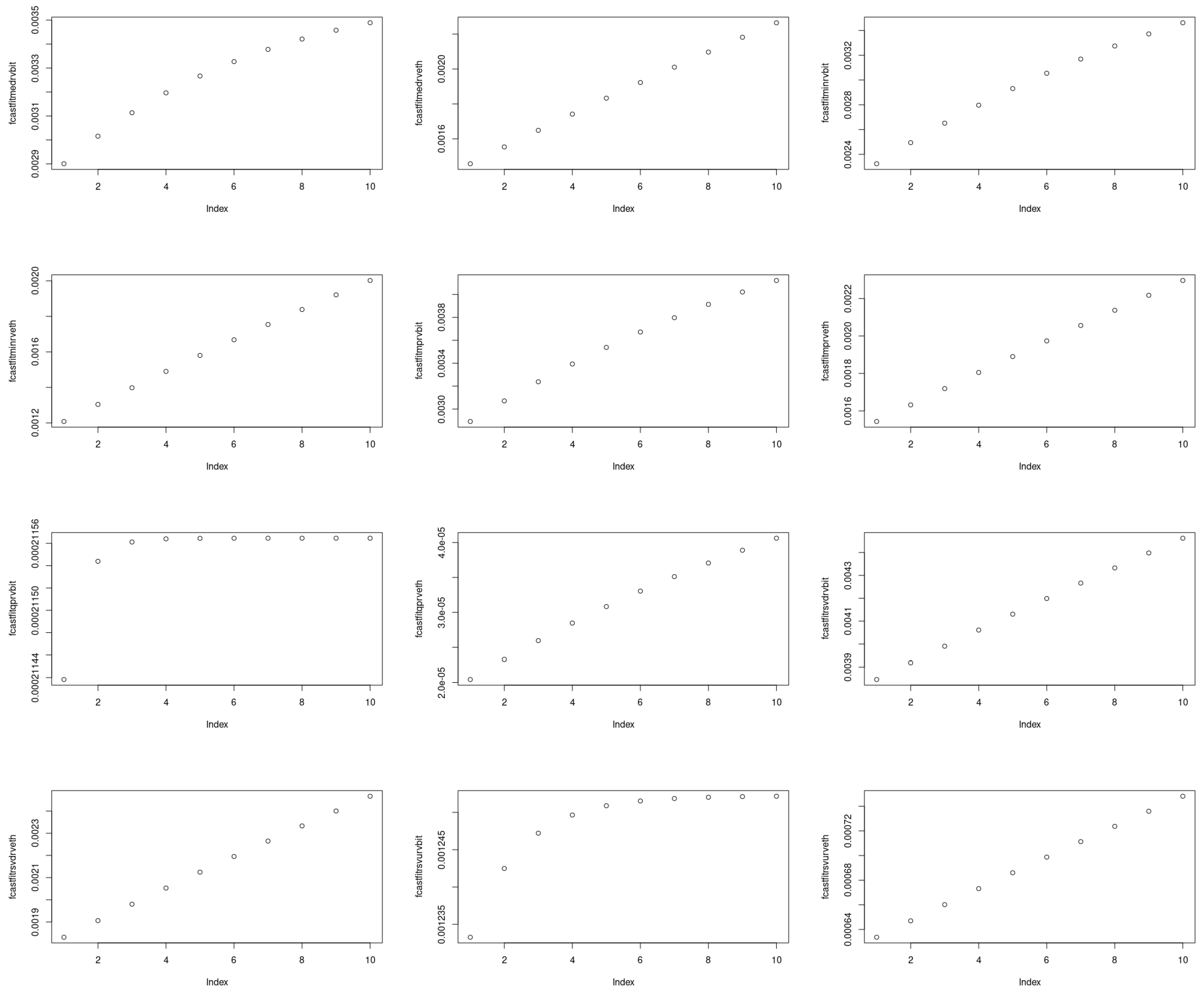
In this paper, we conducted an empirical investigation of the realized volatility of cryptocurrencies using an econometric approach. This work’s two main characteristics are: (i) the realized volatility to be forecast filters jumps, and (ii) the benefit of using various historical/implied volatility indices from brokers as exogenous variables was explicitly considered. We feature a jump-robust extension of the REGARCH-MIDAS-X model incorporating realized beta GARCH processes and MIDAS filters with monthly, daily, and hourly components. First, we estimated six jump-robust estimators of realized volatility for Bitcoin and Ethereum that were retained as the dependent variable. Second, we inserted ten Bitcoin and Ethereum volatility indices gathered from various exchanges as an exogenous variable, each at a time. Third, we explored their forecasting ability based on the MSE and QLIKE statistics. Our sample spanned the period from May 2018 to January 2023. The main result featured the best predictors among the volatility indices for Bitcoin and Ethereum derived from 30-day implied volatility. The significance of the findings could mostly be attributable to the ability of our new model to incorporate financial and technological variables directly into the specification of the Bitcoin and Ethereum volatility dynamics.
1. Introduction
The intrinsic interest of resorting to high-frequency data is to observe the price formation process at the highest frequency available on the exchanges. From that trading signal, options traders, in particular, can take underlying positions in the derivatives markets, typically to hedge or speculate. Another critical characteristic of our work is that we used volatility indices as potential explanatory variables. Be it historical or implied volatility, practitioners indeed pay particular attention to these indices, which serve to gauge the level of ‘fear’ in the markets in the spirit of the VIX (Amendola et al. [1]).
This paper contributes to the extant literature by modeling Bitcoin and Ethereum based on the realized mixed-frequency GARCH model. We enriched the variance dynamics, akin to the GARCH-MIDAS model of Engle et al. [2] and the realized GARCH model of Hansen et al. [3]. Taken together, we implemented a dynamically complete REGARCH-MIDAS-X for Bitcoin and Ethereum with blockchain factors and volatility indices. MIDAS regressions indeed appear to be a particularly attractive approach to the researcher confronted with data sampled at different frequencies, with the idea of parsimony in mind. Whereas the mean reverting daily financial volatility is modeled as a GARCH process, the MIDAS lag polynomials apply to monthly blockchain variables. Therefore, we were able to uncover the short- and long-term components in modeling the volatility of Bitcoin and Ethereum. In this paper, we employed a dataset of intra-daily jump-robust time series, coupled with monthly data for digital variables. To the best of our knowledge, this is the first paper to consider technological factors linked to the blockchain, in addition to volatility indices, as potential drivers of Bitcoin and Ethereum. Consistent with the idea of agents forming expectations of risk from information over varying time horizons, this econometric specification allows modeling a flexible two-component structure for Bitcoin and Ethereum. The short-term component was computed from volatility indices’ series with daily returns, whereas the long-run component was obtained from hashrates with monthly frequency. Linking mean reverting unit daily volatility (through the GARCH process) with monthly technological variables (through MIDAS polynomials) is expected to bring us a wealth of insights. It was hypothesized that including technological variables and volatility indices in the volatility model of Bitcoin and Ethereum will enhance the predictive ability.
There is a burgeoning literature on the REGARCH-MIDAS model. So far, we can limit its writing and applications to just a few groups of authors. On the one hand, Hansen et al. [3] modeled jointly stock returns and realized measures of their volatility and coined it ‘Realized GARCH’ (REGARCH). Unlike the naive augmentation of GARCH processes by a realized measure, the REGARCH model relates the observed realized measure to the latent volatility via the measurement equation. Besides, such a model can capture the dependency over the short term, which should improve the empirical fit (as measured by the log-likelihood or information criteria) and be relevant for forecasting. Applications of the realized GARCH include, to cite a few, Watanabe [4] to quantile forecasts of financial returns, Tian and Hamori [5] for modeling interest rate volatility, Contino and Gerlach [6] to Bayesian tail-risk forecasting, or Bonato [7] to agricultural commodity markets. On the other hand, Borup and Jakobsen [8] retained the short-term dynamics from such a realized GARCH and combined it with MIDAS filters to model the long-term component. More specifically, Borup and Jakobsen [8] initiated the theoretical groundings of the modeling with an illustration of the S&P500 Index and 20 individual stocks. Wu and Xie [9] provided a broader empirical application of the REGARCH-MIDAS to five international stock market indices: the S&P 500, the Nikkei 225, the FTSE 100, the DAX, and the SSE Composite Index. The same group of authors completed their investigation with forecasting exercises of implied volatility on the S&P500 (Wu et al. [10]) and of the VIX (Wu et al. [11]). Wang et al. [12] took a particular interest in the REGARCH-MIDAS model to predict the volatility of China’s New Energy Index comprising 50 companies. Lu et al. [13] resorted to the same kind of modeling to predict the volatility of Chinese agricultural futures markets (i.e., soybean meal, palm oil, corn, soybean oil, soybeans, white sugar, cotton, rapeseed oil, wheat, and rubber).
To the best of our knowledge, only Hung et al. [14] previously studied jump-robust estimators of realized volatility for Bitcoin (not Ethereum), the model with the tri-power variation being the best performer. When comparing jump-robust estimators for the MIB, DAX, CAC, and FTSE stock markets, Čuljak et al. [15] documented empirically the superiority of the two time scale version. In comparison, this paper scrutinized up to six jump-robust estimators of the realized volatility for Bitcoin and Ethereum. It is crucial that the econometric analysis distinguishes between the continuous and jump components of realized volatility based on the advances in the financial econometrics literature (see, e.g., initially, Andersen et al. [16] or, more recently, Caporin [17]). Also, jumps are very prevalent in the tick data of Bitcoin and Ethereum, as high as 25%, as previously detected by Sanhaji and Chevallier [18]. Taken together, these two arguments offer a proper justification to push the research effort one step further.
The main contribution to the literature on cryptocurrency markets is to propose a hybrid frequency approach that collapses intra-daily, daily, and monthly data in the vein of the High-Frequency Data-Based Projection-Driven GARCH by Chen et al. [19] and Chen et al. [20]. We propose an innovative approach based on the REGARCH-MIDAS-X tailored to jump-robust estimators of Bitcoin and Ethereum realized volatility combined with each cryptocurrency’s hashrate (as the MIDAS filter) and up to ten historical/implied volatility indices (as the explanatory ‘X’ factor). The research question deals with the jump-robust high-frequency analysis of Bitcoin and Ethereum with the exogenous informational content of volatility indices. The building blocks of REGARCH-MIDAS-X are gradually explained in the paper. To the best of our knowledge, we are the first empirical attempt at including digital (stemming from blockchain) and financial (stemming from options) variables as exogenous variables to explain Bitcoin and Ethereum returns in such a high-frequency jump-robust GARCH-MIDAS framework. We considered models with one explanatory variable at a time, over the six jump-robust estimators, and conducted as well a multi-day-ahead forecasting exercise. Our sample spans from May 2018 to January 2023.
To provide a gist of the results, the performance of REGARCH-MIDAS-X depends on the choice of explanatory variables. According to our experiments, the model with 30-day implied volatility as an exogenous driver was the best choice. This result was stable for the six classes of jump-robust estimators considered. Disentangling between the short-term GARCH volatility and the long-term MIDAS filters also led to better out-of-sample predictive ability of Bitcoin and Ethereum volatility. The intuition behind this finding is the information flows at different frequencies and with various degrees of persistence (Adrian and Rosenberg [21]). Daily news is short-lived on financial markets and can be deemed as ‘high-frequency’ (Calvet and Fisher [22]). On the contrary, monthly changes in technological conditions appear at a lower frequency and exhibit a longer-lasting impact. Our results are useful for selecting the appropriate drivers of Bitcoin and Ethereum. The performance of REGARCH-MIDAS-X depends indeed on the choice of the explanatory variables. The best specification was achieved by including 30-day implied volatility series. We concluded that adding information from derivatives options to a REGARCH-MIDAS-X model can improve the model’s forecasting performance. The findings can have implications for hedging investment and risk management as well.
The remainder of the article is structured as follows. Section 2 outlines the various classes of jump-robust estimators mobilized from high-frequency data for Bitcoin and Ethereum. Section 3 lays out the building blocks of the REGARCH-MIDAS-X models. Section 4 details the ten volatility indices retained for Bitcoin and Ethereum as explanatory variables. Section 5 contains the results from the REGARCH-MIDAS-X estimates and the associated forecasts. Section 6 concludes.
2. Jump-Robust Estimators of Realized Volatility for Bitcoin and Ethereum
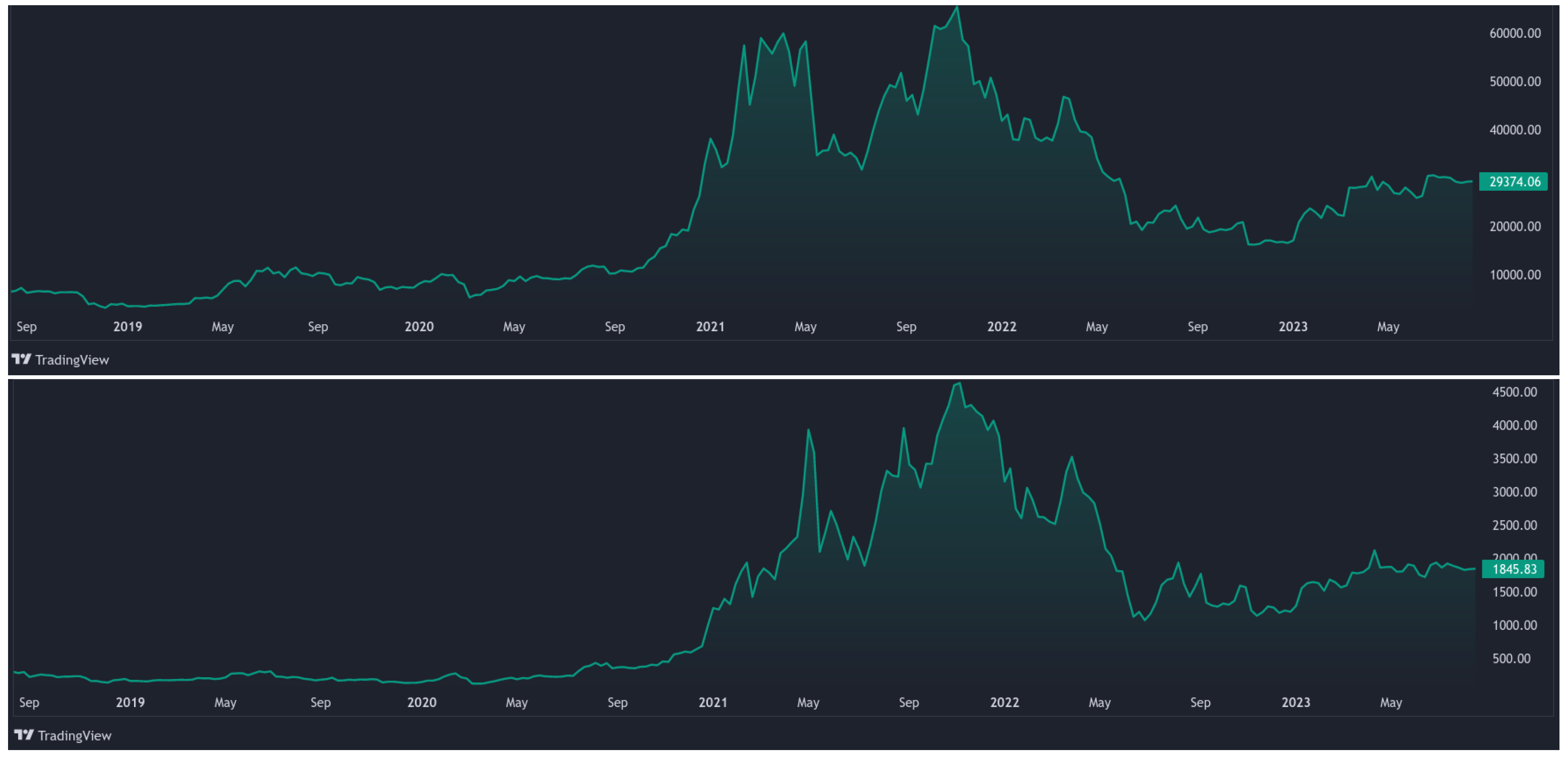
The price series (in levels) of Bitcoin and Ethereum are shown in Figure 1 from TradingView (see https://www.tradingview.com/chart/?symbol=CRYPTO%3ABTCUSD (accessed on 14 August 2023) for BTC and https://www.tradingview.com/symbols/ETHUSD/?exchange=CRYPTO (accessed on 14 August 2023) for ETH.). These underlying securities serve as the basis of our empirical application.
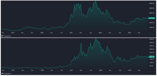
Figure 1.
TradingView’s 5-year BTCUSD (top) and ETHUSD (bottom) charts.
The tick data with a 60 min frequency for Bitcoin and Ethereum were sourced from CryptoData Download, more specifically by selecting the Bitfinex exchange, which is the most-liquid for derivatives (see, e.g., Alexander et al. [23] and Alexander and Dakos [24], Alexander and Heck [25]). The sample size is equal to 1709 observations from 15 May 2018 to 17 January 2023.
Sanhaji and Chevallier [18] documented that microstructure noise is present in Bitcoin and Ethereum high-frequency data for up to 4 min. This is on par with previous studies on the S&P500 documenting the presence of microstructure noise up to 5 min (see, e.g., Martens [26], Huang et al. [27]). Therefore, we considered that our paper will not be plagued by microstructure noise, given that we downloaded the data at a 60 min frequency (e.g., hourly data).
Since Sanhaji and Chevallier [18] already documented the properties of ‘naive’ Realized Volatility (RV) for Bitcoin and Ethereum, we focused instead in this article on extending the realm of investigation to the class of jump-robust estimators of RV. More specifically, we considered six jump-robust estimators for Bitcoin and Ethereum:
- MedRV;
- MinRV;
- Realized MultiPower Variation;
- Realized QuadPower Variation;
- Realized Semi-Variance Downside;
- Realized Semi-Variance Upside.
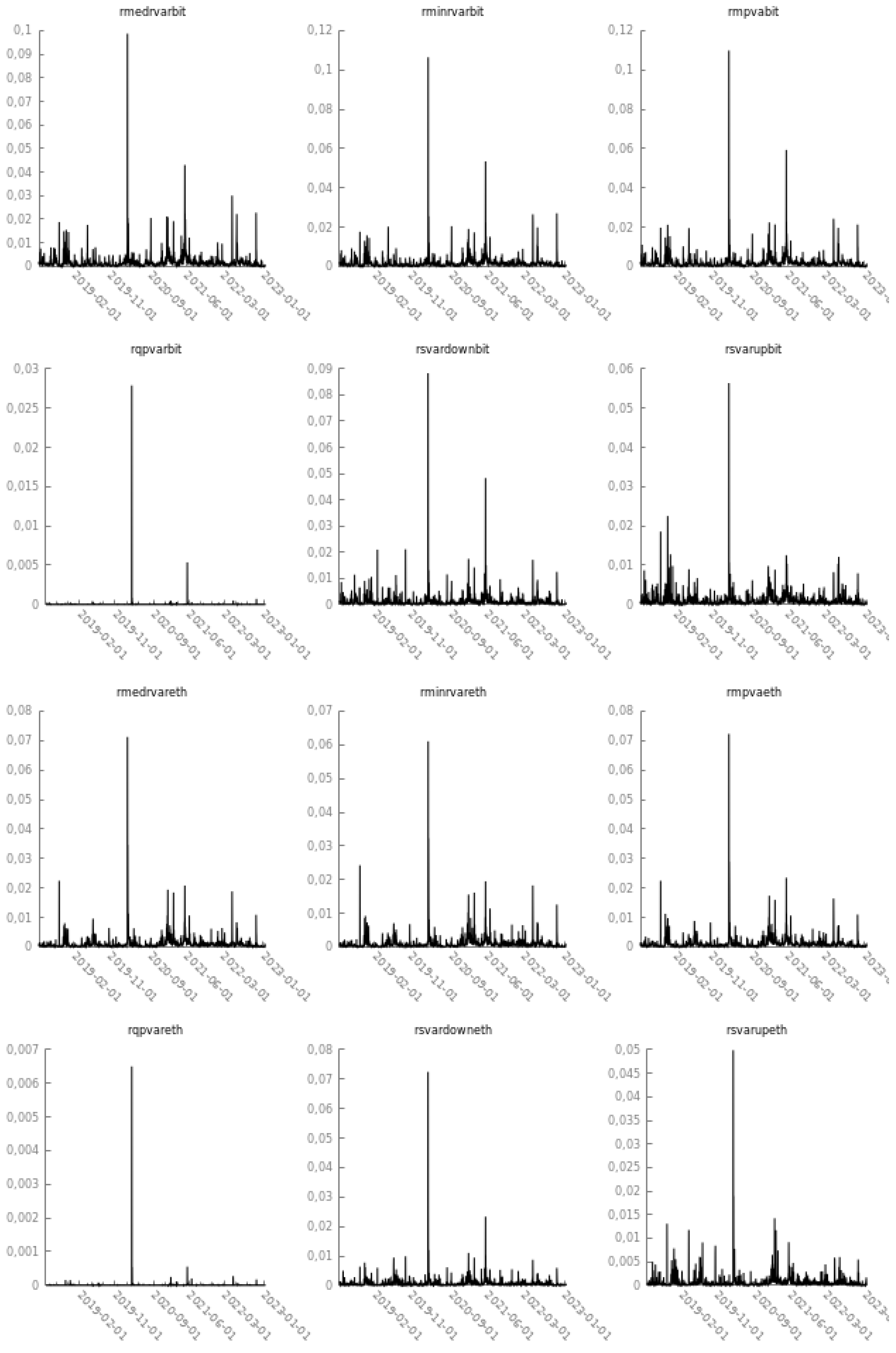
These can be viewed in Figure 2. These series will be specified iteratively as the dependent variable in REGARCH-MIDAS-X. The corresponding descriptive statistics can be found in Table A1 of Appendix A.

Figure 2.
Jump-robust estimators for Bitcoin and Ethereum from 15 May 2018 to the present. Note: For Bitcoin, is the MedRV estimator, the MinRV estimator, the RMPV estimator, the RQPV estimator, the RSV-down estimator, and the RSV-up estimator. The corresponding estimators are indexed by eth for Ethereum.
We borrowed the notations from Andersen et al. [28] in the theoretical exposition. Consider the univariate logarithmic price process of an asset. The price process is observed at the discrete points in time over a given period, which we refer to as a trading day. The corresponding returns and time intervals are denoted and , . For simplicity, assume equally spaced sampling, i.e., , for all . With regard to asymptotics, the time increments between successive return observations, defining the sampling scheme, uniformly shrink towards zero as N increases.
Next, consider the classic jump-diffusive representation:
where is a locally bounded and predictable process and is a càdlàg and bounded away from zero almost surely. In order to properly disentangle the continuous and jump components, stands for the standard Brownian motion (or Wiener process). J denotes a finite activity jump process, and is either zero (no jump) or a real number indicating the occurrence and size of a jump at time t. Notice that our strategy naturally discards the RV estimator, which would estimate the total quadratic variation of the observed semimartingale, including the contribution from the cumulative squared jumps.
In this paper, we really needed to estimate the Integrated Variance (IV), defined as . To achieve this task, we started with the first two MinRV and MedRV estimators of integrated variance:
The scaling factors ensure that every summand on the right-hand side of the equation provides an unbiased estimate of the underlying spot variance if the corresponding returns block is i.i.d. Gaussian. The interest behind the MinRV and MedRV estimators stems from the min/med operators fully eliminating returns contaminated by a large jump. Andersen et al. [28] demonstrated that the MinRV and MedRV estimators are indeed consistent for the IV.
Third, Andersen et al. [28] generalized the class of Realized MultiPower Variation (RMPV) statistics, defined via the cumulative sum of m products of adjacent absolute returns raised to the th order, where m is a positive integer and r a positive real number, usually an integer. Hence, the cumulative power of the adjacent products equals r. In the numerical implementation of RMPV, the window size of return blocks was set equal to 2 by default. Similarly, the power of the variation was set equal to 2 by default. These statistics provide consistent estimators for the corresponding integrated power of the volatility:
where is a known constant dependent only on m and r, while is a finite-sample-correction factor. If the adjacent returns are i.i.d. Gaussian, each summand in the equation delivers an unbiased estimate of the power of spot volatility. The sum, therefore, provides a (converging) Riemann approximation to the integrated power of the volatility process. In this context, RMPV effectively generalizes the entire first generation of estimators in the realized volatility literature.
Fourth, it is, therefore, immediate to derive the Realized QuadPower Variation as:
In the presence of a finite activity jump process, the additional benefit of the QuadPower measure is to allow an associated asymptotic mixed normal limit theory.
Last, but not least, we considered two additional jump-robust estimators originating from Barndorff-Nielsen et al. [29]. We now follow the notations from Bollerslev et al. [30], who assumed that high-frequency intraday prices are observed at equally spaced times over the trading day . Furthermore, Bollerslev et al. [30] denoted the natural logarithmic discrete-time return over the ith time-interval on day by .
According to these latest notations, the fifth Realized Downside Semi-Variance (RSV-down) and sixth Realized Upside Semi-Variance (RSV-up) estimators decompose the total realized variation into separate components associated with the positive and negative high-frequency returns:
For practical applications, think of RSV-down as a new source of information that focuses on squared negative jumps. Conversely, RSV-up may be of particular interest to investors with short positions in the market (hence, a fall in price can lead to a positive return and, hence, is desirable), such as hedge funds. Moreover, it is possible to show that:
such that the separately defined positive and negative semi-variance measures converge to one-half of the integrated variance plus the sum of squared positive and negative jumps, respectively. These limiting results imply that the difference between the semi-variances removes the variation due to the continuous component and, thus, only reflects the variation stemming from jumps. Bollerslev et al. [30] referred to this ‘good’ minus ‘bad’ realized volatility measure as the signed jump variation.
In the next section, we consider how to plug these six jump-robust estimators of realized volatility for Bitcoin and Ethereum, which we display in Figure 2, as the dependent variable into the REGARCH-MIDAS-X model.
3. Building Blocks of the Realized GARCH-Mixed Data Sampling-X Model
For methodological purposes, we detail the econometric methodology and the various estimation tasks step-by-step.
3.1. Objectives of the Model
Looking at the evolution of the prices of any asset, a good understanding of the evolution of the associated volatility is essential. GARCH processes (Engle [31], Bollerslev [32]) allow the extraction of information about the current level of volatility. Nevertheless, the current level of volatility based on the squared returns can appear as poor information when this volatility changes rapidly to a new level. Thus, a GARCH process is slow at catching these changes.
If the assets are known by their daily prices, the GARCH models give information on the volatility of these daily prices. The recent availability of high-frequency data (second, minutes, etc.) has caused researchers to introduce new measures of volatility called realized measures of volatility, which were introduced into the GARCH modeling. Thus, Hansen et al. [3] introduced the Realized GARCH (REGARCH) model in 2011. These REGARCH models have provided an advantageous structure for the joint modeling of stock returns and realized volatility measures.
According to Andersen et al. [33], the exploitation of granular information in high-frequency data by considering realized measures constitutes a much stronger signal of latent volatility than squared returns. However, with this approach, we do not capture the existence of the dependence structure characterized by a positive and slowly decaying autocorrelation function or a persistence parameter close to unity (the famous ‘integrated’ GARCH effect). A multiplicative decomposition of the conditional variance into a short-term and a long-term component has been developed to capture the evident high persistence.
In 2019, Borup and Jakobsen [8] modeled the short-term component via a first-order REGARCH model and the long-term component via, for instance, a MIxed-DAta Sampling (MIDAS) structure. In this long-term component, several MIDAS variables can be taken into account. Typically, they could be macro variables like global financial stress indexes, some economic policy uncertainty indexes known at a monthly frequency, or financial variables like the monthly realized volatility computed through the daily realized variances.
In this paper, we aimed to understand better the evolution of Bitcoin and Ethereum price swings observed within a day. Thus, we investigated the volatility of these crypto assets by looking simultaneously at the evolution of their latent volatility based on daily returns with long- and short-term components, as well as their jump-robust realized volatility based on high-frequency data (60 min). With the perspective of a long-term forecasting horizon, we are interested in detecting the drivers behind these cryptocurrency assets by considering the existence of persistence in their volatility.
We proceed with a brief exposition of the REGARCH-MIDAS-X model to answer these different expectations. A full-fledged version can be found in Borup and Jakobsen [8].
3.2. Some Notations
Let denote a time series of returns, a time series of realized measures, and a filtration so that is adapted to . We define the conditional mean and the conditional variance . We now introduce the specific modeling for introducing several time scales that we used in terms of low and high frequencies.
We define the daily returns , where is the price of the asset. In the MIDAS framework, it is convenient to introduce two time scales: here, denotes the monthly frequency and the number of days within a month t, (Typically, to amount to the number of days traded within a month. m can be formulated either via keeping it locally constant or else based on a local moving window. Engle et al. [2] documented that the difference between the two is negligible.) We assumed that the conditional mean corresponds to a zero-beta portfolio (Black [34]):
with
The innovation is assumed to be i.i.d. with mean zero and variance one (The innovation is an i.i.d random variable from a Student’s t distribution with degrees of freedom, as fat-tailed distributions are found adequate to describe financial data (Kuester et al. [35]).); and denote the short- and long-term components of the conditional variance, respectively.
The short-term component varies at the daily frequency and follows a unit variance GARCH(1,1) process. We used a logarithmic specification, which automatically ensures a positive variance:
where , , and .
The specification of the long-term (secular, low-frequency) volatility component builds on a long tradition, dating back to Merton [36] and Schwert [37], of measuring long-run volatility by realized volatility over a monthly horizon. What is new here is that is specified by smoothing historical realized volatilities in the spirit of MIDAS filtering, instead. Accordingly, the long-term component is regressed on a set of variables, varies at the monthly frequency, and is given by:
where and K is the number of periods over which the variables are smooth. denotes the MIDAS variable at the monthly frequency. assigns the importance of the MIDAS variable. z is the parameter accounting for the statistical significance of the volatility index inserted one at a time as an exogenous explanatory variable in our REGARCH-MIDAS-X experiments.
The parameter depicts a selected weighting scheme. This procedure allowed us to estimate optimally the number of lags for both the daily and monthly returns within MIDAS. It can produce various lag structures for past returns, monotonically increasing/decreasing, hump-shapes, etc. Ghysels et al. [38] documented that the beta function is a better choice than the exponential Almon for high-frequency models. In our setting, we, therefore, introduced:
By construction, the weights , , sum to one. Practically, we imposed , which implies that the weights are monotonically declining.
We now introduce the realized measure of volatility , inside the measurement equation, which provides a framework for the joint modeling of returns and volatility based on high-frequency data. Specifically, this paper features jump-robust estimators (sampled at an hourly frequency to avoid microstructure noise; see, e.g., Hansen and Lunde [39]) of Bitcoin and Ethereum instead of the naive RV, as recalled in Section 2 (see Sanhaji and Chevallier [18] for a further reference).
Unlike the naive augmentation of GARCH processes by realized measures, the REGARCH model relates the observed realized measure to the latent volatility via the measurement equation. According to Hansen et al. [3], including the realized measure in the model and the fact that has an ARMA representation motivate its name. In what follows, t denotes the daily frequency and i is the hourly frequency:
The sequence was assumed to be i.i.d. with mean zero and variance , and being mutually independent. Equation (12) is natural when is a consistent estimator of the integrated variance. The innovation is captured by .
is called the leverage function. This function captures the dependence between returns and future volatility, and we used the functional form constructed on Hermite polynomials, i.e.,:
The choice of Hermite polynomials is retained here, permitting a simple quadratic form, ensuring with and for any distribution. This form generates an asymmetric response in volatility to returns shocks, permitting mapping out how positive and negative shocks to the price affect future volatility. The parameter reflects how much the daily volatility occurs during trading hours. The parameters and (for instance) show how a shock in the price impacts volatility. For that, we can use the impact curve defined as . So, measures the percentage impact on volatility as a function of a return shock: .
To sum up, Equation (7) is labeled as the ‘return equation’, Equation (9) as the ‘GARCH equation’, Equation (10) as the ‘long-term’ equation, Equation (11) as the ‘weighting scheme’, and Equation (12) as the ‘measurement equation’. In this multiplicative framework, the ‘GARCH equation’ drives the dynamics of latent volatility. The ‘measurement equation’ is the true innovation in REGARCH and makes the model dynamically complete. It links the ex post realized measure with the ex ante conditional variance. It facilitates a simple modeling of the dependence between returns and future volatility. Of course, discrepancies between the two measures can be observed in . On the one hand, the conditional variance refers to close-to-close market intervals (e.g., daily returns). On the other hand, the realized measure is computed from open-to-close market intervals (in our setting, hourly sampling frequency). That is why both proportional and exponential correction parameters are included.
3.3. Estimation Practicalities
In the tables of results, the parameter space will be synthetically reproduced as with distributional assumptions and . and were assumed to be mutually and serially independent. Hansen et al. [40] further detailed the decomposition of the conditional density, leading to two contributions to the log-likelihood function. Empirically, the model is estimated by the Quasi-Maximum Likelihood Estimator (QMLE).
The asymptotic analysis of the quasi-maximum likelihood estimator for the GARCH MIDAS model can be found in Wang and Ghysels [41]. They provided a rigorous analysis of the maximum likelihood estimator of the GARCH-MIDAS model, so that it admits covariance stationary or strictly stationary ergodic solutions or satisfies -mixing properties. Besides, they documented that the QMLE is unbiased and the asymptotic standard errors are valid in the presence of exogenous explanatory variables.
For the realized GARCH, Hansen et al. [3] and Hansen and Huang [42] detailed the regularity conditions that justify the QMLE’s inference. They noticed that the mathematical structure of the log-likelihood function for the realized GARCH is similar to the structure analyzed in Straumann et al. [43], who adopted a stochastic recurrence approach to analyze the QMLE properties for a broad class of GARCH models. Besides, they relied on their proof of previous works by Jensen and Rahbek [44] and Jensen and Rahbek [45], documenting that the QMLE is consistent with a Gaussian limit distribution regardless of the process being stationary or non-stationary. Regarding the theoretical properties of the log-linear specification in the realized GARCH, Hansen et al. [3] provided closed-form expressions for the first and second derivatives of the log-likelihood function that enable the computation of robust standard errors (An attractive feature of the log-linear representation is that it conveniently preserves the ARMA structure that characterizes the GARCH equation. Another advantage of using a logarithmic form is that it automatically ensures a positive variance. Hansen et al. [3] presented additional evidence in favor of the log-linear specification in Section 5.5 of their paper.).
Based on previous works by Han and Kristensen [46], Han [47], and Francq et al. [48], Borup and Jakobsen [8] further documented the log-likelihood function of REGARCH-MIDAS:
In Equation (14), the joint log-likelihood is split into a sum of univariate models, whose likelihood can be maximized separately. The factorization of the likelihood is possible because:
- All observables are tied to their individual latent volatility process (e.g., is tied directly to the conditional volatility );
- The innovations and are taken to be independent in the formulation of the likelihood function.
Borup and Jakobsen [8] proceeded to calculate the score functions as a martingale difference sequence, which defines the first-order conditions for the maximum-likelihood estimator and facilitates the direct computation of standard errors for the coefficients. Specifically, for the long-run component, the derivatives for REGARCH-MIDAS can be found in Equation (A.41) of their Supplementary Appendix. To check the validity of the asymptotic distribution of the estimators, Borup and Jakobsen [8] followed the parametric bootstrapping technique by Paparoditis and Politis [49]. The in-sample distribution of the estimated parameters for REGARCH-MIDAS aligns with a normal distribution. The authors concluded that the QMLE approach and associated inferences are valid.
In terms of estimation ‘tricks’, we initialized the conditional variance process to be equal to its unconditional mean. To initialize the long-term component , we set the past values of equal to for the length of the backwards-looking horizon in the MIDAS filter. To avoid the issues of inferior local maxima during the estimation, we considered a grid of starting values by perturbation. Given this perturbation, the numerical optimization was stable. Currently, the estimation of MIDAS filters is eased by several licensed (e.g., Matlab, Eviews) or GNU (R CRAN, Octave, Gretl) software, with resources flagged on Eric Ghysel’s website (http://eghysels.web.unc.edu/ (accessed on 13 January 2023) (Onno Kleen and Daniel Borup also will provide their respective codes upon request to them.).
3.4. Selecting the Mixed Data Sampling Filter: Cryptocurrency Hashrates
Since the seminal contribution by Ghysels et al. [50], the appeal of MIxed DAta Sampling (MIDAS) has been immediate to all macroeconomists (Ghysels et al. [38] defined the MIDAS regressions as “a simple, parsimonious, and flexible class of time series models that allow the left-hand and right-hand variables of time series regressions to be sampled at different frequencies”.). It offers, indeed, the possibility to contrast the frequency available in financial markets (typically, daily or intraday) with that available for macroeconomic variables (e.g., quarterly or monthly). By using the highest frequency available for each series, the econometrician is, therefore, not losing any information, as he/she would have in the case where he/she had harmonized all the series (say, to monthly frequency) to obtain a balanced sample. Initial applications of this technique include, to cite a few, Ghysels et al. [51], who found a significantly positive relation between the conditional mean and the conditional variance of the aggregate stock market return, or Ghysels et al. [52], who considered various MIDAS regressions to predict volatility. A survey can be found in Ghysels et al. [38].
MIDAS consists of two additive components, one interpreted as a short-run (transitory) component estimated with daily return data and a second one identified as the long-run (secular trend) component obtained from macroeconomic monthly data. Alternatively, the short-term part could reflect the day traders’ investment horizon. In contrast, the long-term component could relate to pension funds or other types of investors with longer-term maturities in mind. Katsiampa [53] documented that Bitcoin volatility can indeed be decomposed into short- and long-term components. Once again, we observed the ability of the component models to capture complex dynamics via a parsimonious parameter structure.
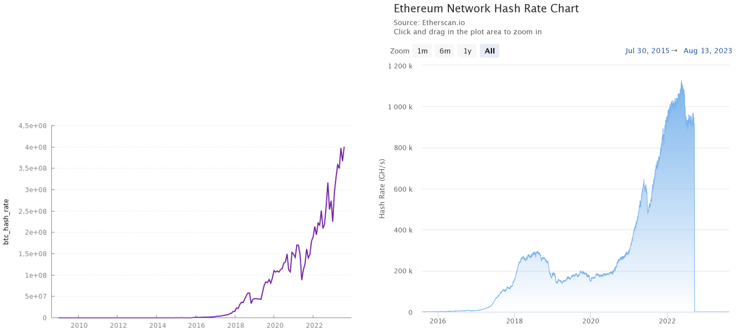
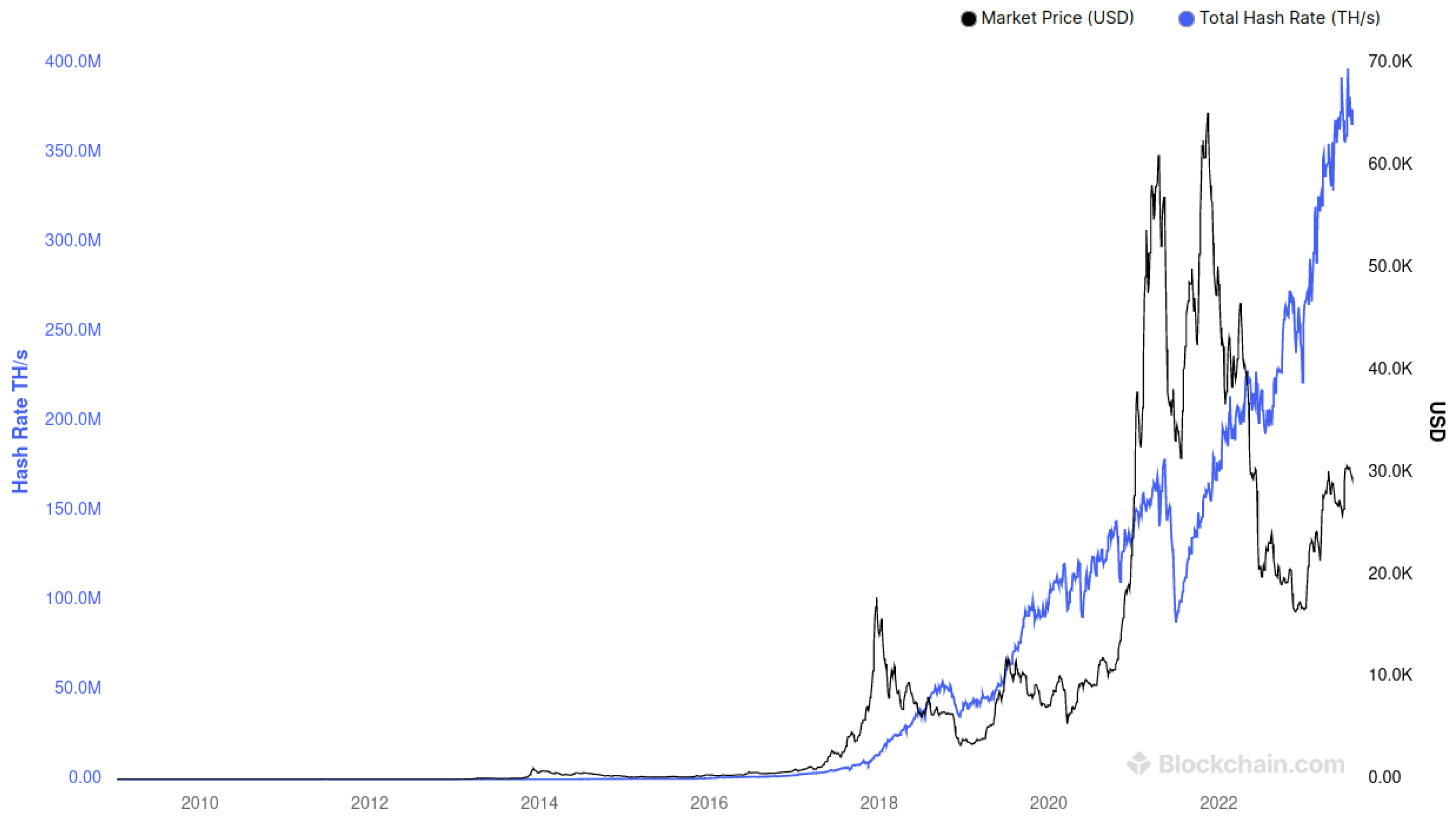
Regarding the long-term MIDAS macro component serving as a proxy of the business cycle, the monthly industrial production is typically selected by studies on the S&P 500 index (see, e.g., Engle et al. [2] or Conrad and Loch [54]). In this paper, we opted for a more ‘digital’ MIDAS filter by selecting the hashrate, which shows the historical measure of the processing power on a given blockchain network. For instance, Bitcoin’s market price and total hashrate tend to go hand in hand (see, e.g., Fantazzini and Kolodin [55], Marthinsen and Gordon [56], and Kubal and Kristoufek [57]), as is visible to the interested reader in Figure A1 of Appendix A. Bitcoin’s monthly hashrate was sourced from Nasdaq Data Link. Ethereum’s hashrate was sourced from Etherscan. Both variables are displayed in Figure 3. The ‘digital’ MIDAS filter was transformed to a logarithmic first difference.
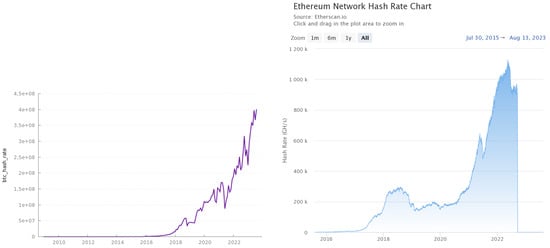
Figure 3.
Nasdaq Data Link’s monthly hashrate for Bitcoin from 31 January 2009 to the present (left) and Etherscan’s Ethereum hashrate from 30 July 2015 to the present (right).
4. Volatility Indices for Bitcoin and Ethereum: The ‘X’ Factor
This section details the (10×) Bitcoin and Ethereum volatility indices that will be used as the ‘X’ in the REGARCH-MIDAS-X model in the subsequent estimation and prediction steps.
4.1. Historical Volatility Indices
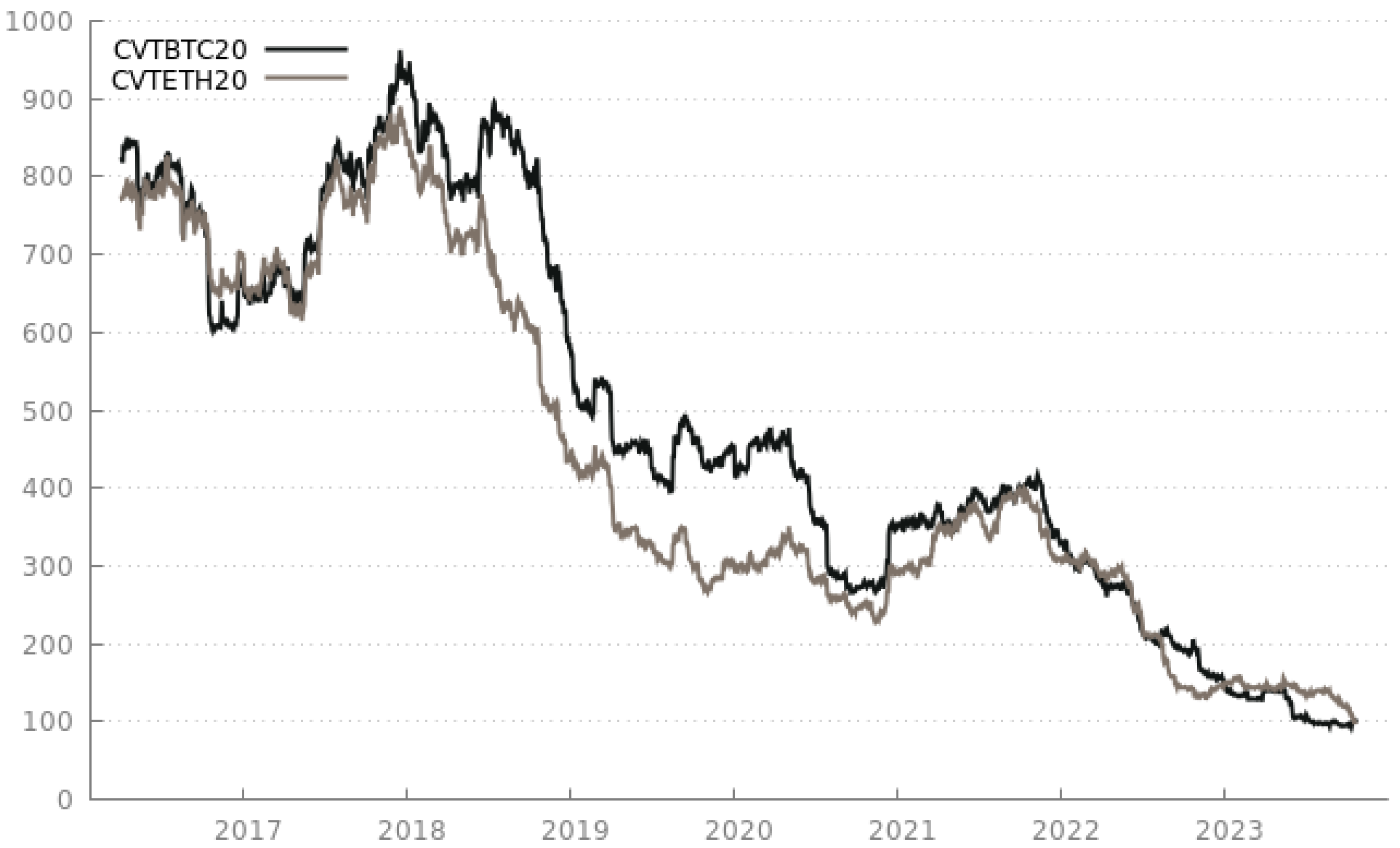
Compass Financial Technologies proposes a wide array of Crypto Volatility Target Indices. Two of them are of particular interest to us in this paper. On the one hand, we have the Compass Crypto Volatility Index Bitcoin 20% (CVTBTC20), computed from Kaiko’s historical tick-by-tick trade data, whose annualized historical volatility target algorithm is set at 20%. On the other hand, we find the Compass Crypto Volatility Target Index Ethereum 20% (CVTETH20), which exhibits similarly an annualized volatility target of 20% by functioning on rolling windows (Compass FT’s methodology is available at https://www.compassft.com/wp-content/uploads/CCVT$_$Methodology.pdf (accessed on 13 August 2023)). Both Bitcoin- and Ethereum-based indices from Compass FT are available from 4 February 2016 onwards. The Compass BTC and ETH Target Volatility Indices are shown in Figure 4.
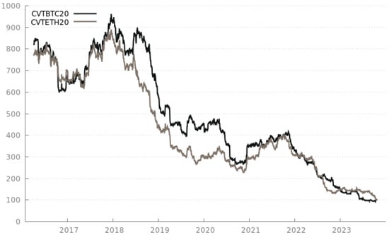
Figure 4.
Compass FT’s CVTBTC20 and CVTETH20 from 4 February 2016 to the present.
Next, Bitcoinity has created a Bitcoin Price Volatility Index from various exchanges. We chose Bitfinex as one of the most-liquid crypto exchanges, especially for derivatives. The index is computed as the standard deviation from all market trades, in logarithmic form, with a moving average smoothing. Bitcoinity’s index has been computed since 10 March 2013. It is shown in Figure 5.
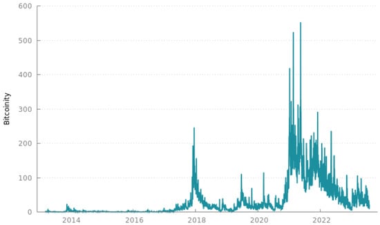
Figure 5.
Bitcoinity’s Bitcoin Price Volatility Index from 10 March 2013 to the present.
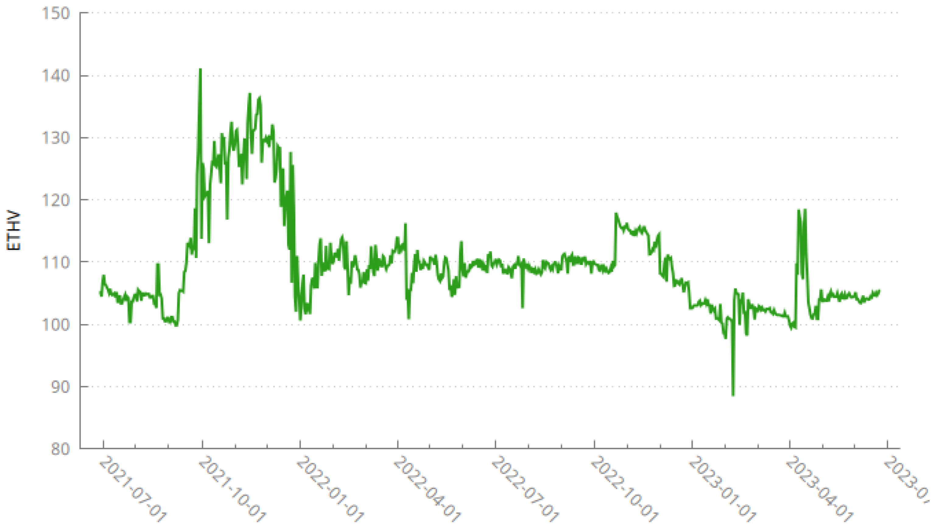
Regarding Ethereum, Volmex Labs Finance calculates the Ethereum Volatility Index (ETHV) to track Ethereum’s expected historical volatility over the next 30 days. This token has been available on several exchanges like CoinGecko since 28 June 2021. It is reproduced in Figure 6.

Figure 6.
Volmex Labs Finance’s ETHV from 28 June 2021 to the present.
4.2. Implied Volatility Indices
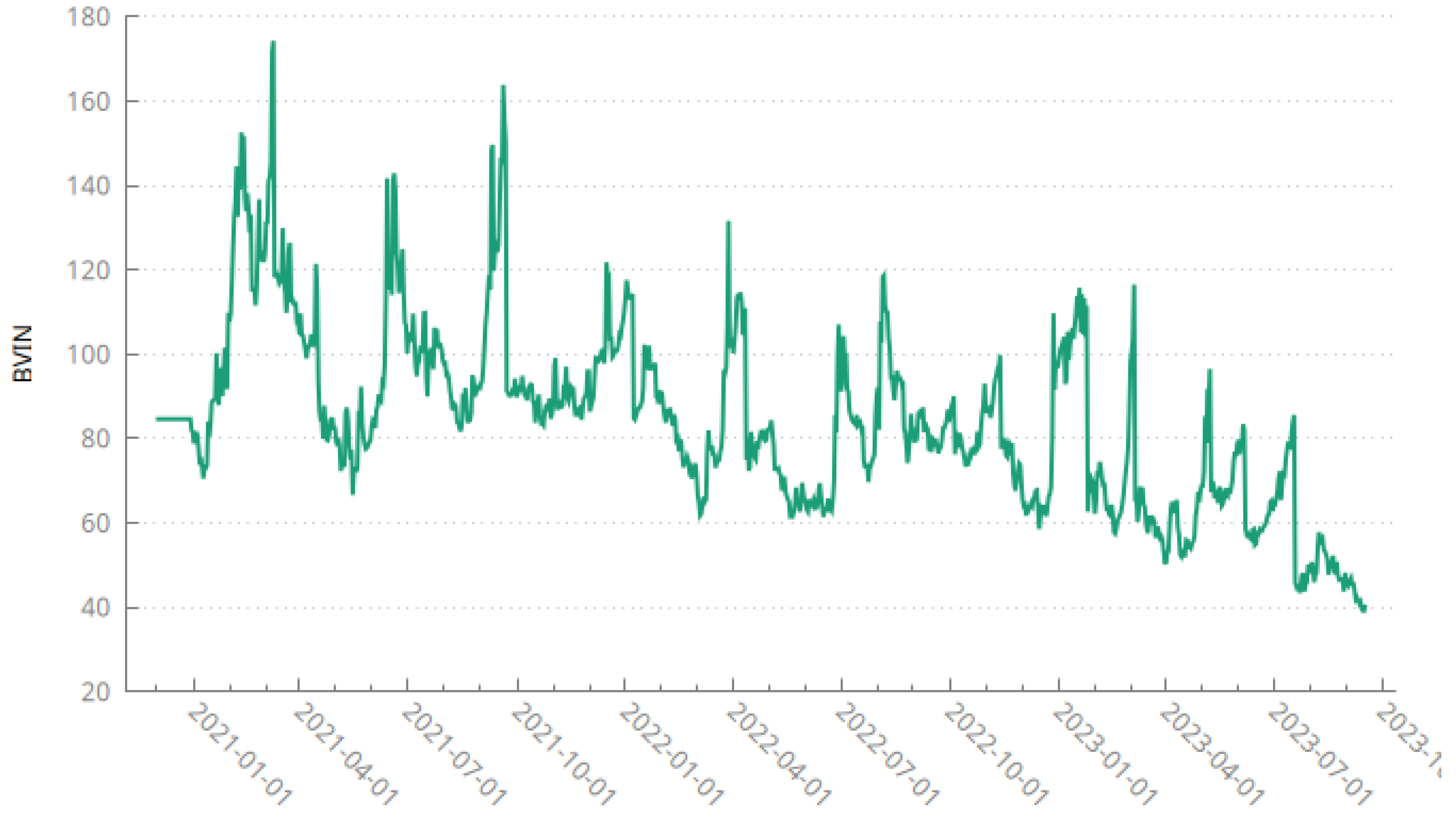
Alexander and Imeraj [58] constructed their own Bitcoin VIX, by following the same methodology as the original CBOE’s VIX. The index is calculated using 30-day Bitcoin options data from the broker Deribit. Their index is now registered on Cryptocompare under the BVIN (Bitcoin Volatility Index) ticker. This volatility index is available from 1 December 2020 onwards. It is reproduced in Figure 7.
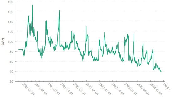
Figure 7.
The Bitcoin Volatility Index (BVIN) from 1 December 2020 to the present.
Next, Triple3 Partners have proposed both the BitVol (Bitcoin Volatility) and EthVol (Ethereum Volatility) indices measured from 30-day implied volatility on at-the-money options for BTC and ETH, respectively (the T3Index documentation is available at https://t3index.com/wp-content/uploads/2022/06/Bit-Vol-process$_$guide-Jan-2019-2022$_$03$_$22-06$_$02$_$32-UTC.pdf (accessed on 13 August 2023)). These volatility indices are available from 8 January 2019 onwards for BTC and from 15 April 2020 onwards for ETH. They are reproduced in Figure 8.
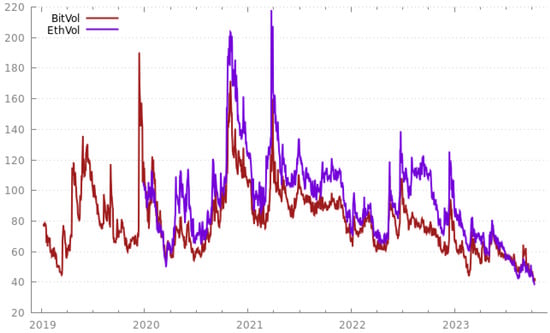
Figure 8.
Triple3 Partners’ BitVol and EthVol from 8 January 2019 to the present.
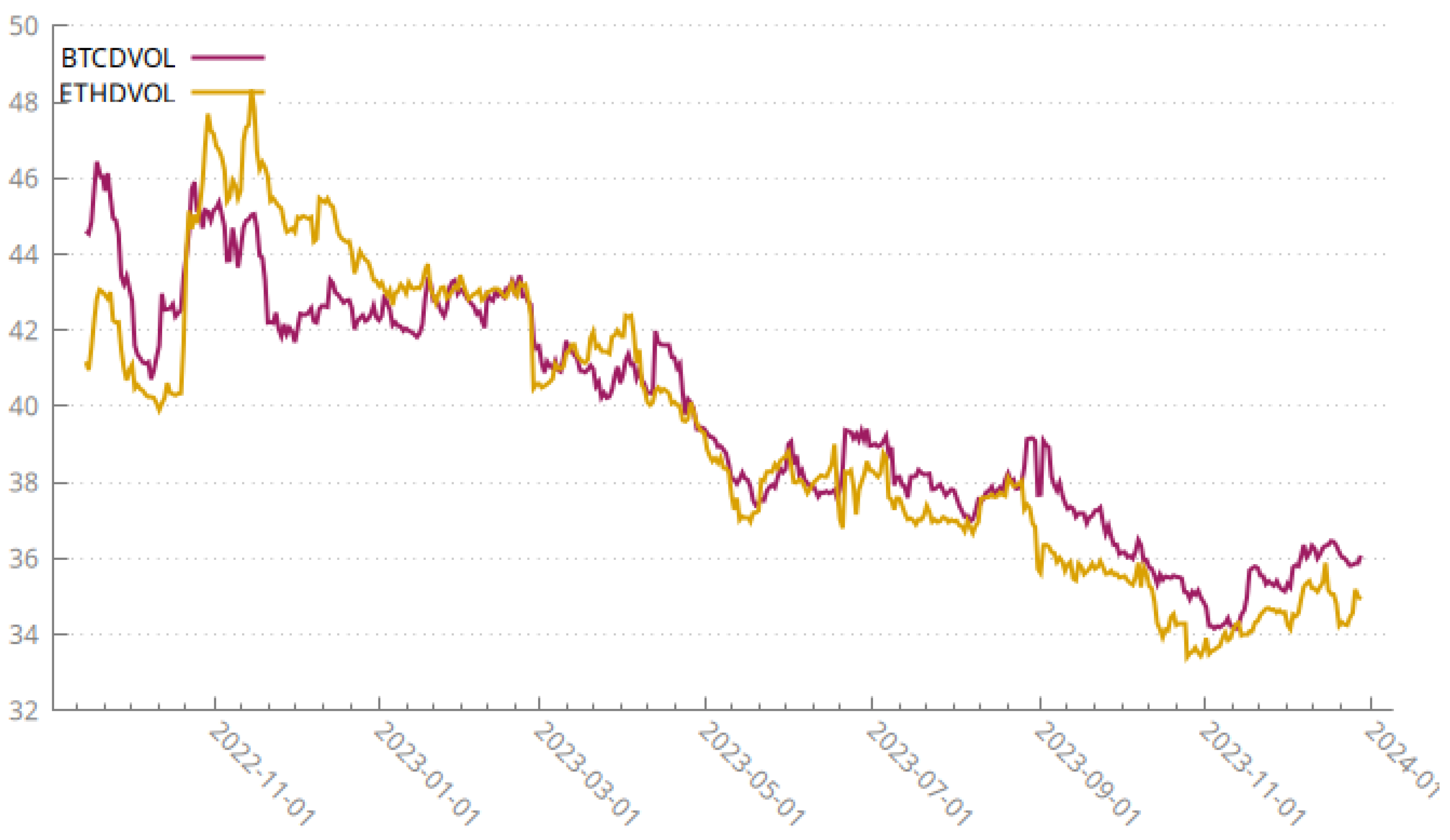
As a broker, Deribit also proposes its own custom BTC and ETH Volatility Indices (DVOLBTC and DVOLETH, respectively). Their methodology also hinges on a 30-day implied volatility from options (the Deribit documentation is available at https://insights.deribit.com/industry/demystifying-dvol-futures/ (accessed on 13 August 2023)). The Deribit Volatility Indices are available from 26 March 2023 onwards. The Deribit Volatility Indices are visible in Figure 9.

Figure 9.
Deribit’s DVOLBTC and DVOLETH from 26 March 2023 to the present.
4.3. Aggregate Cryptocurrency Volatility Indices
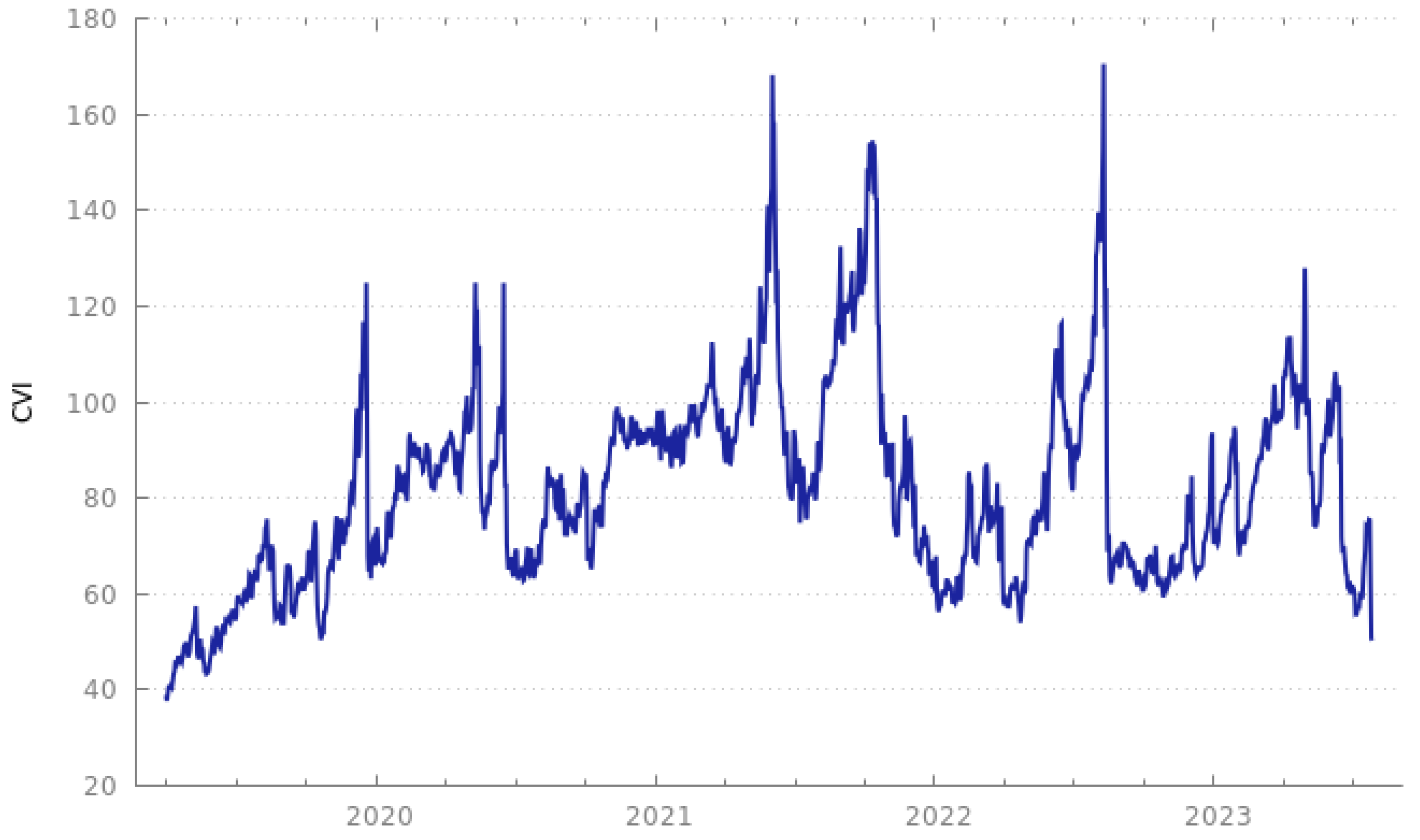
The Crypto Volatility Index (CVI) is advertised as ‘the VIX of Crypto’ by CVI Finance. As for the original VIX, the goal is to estimate the 30-day implied volatility based on the Black–Scholes options pricing model tailored for Bitcoin and Ethereum options (the CVI documentation is available at https://docs.cvi.finance/cvi-index/index-calculation (accessed on 13 August 2023)). The CVI is available on Investing.com from 31 March 2019 onwards. It is pictured in Figure 10.
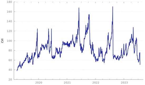
Figure 10.
CVI Finance’s Crypto Volatility Index from 31 March 2019 to the present.
There used to be another competitor for the VIX of the whole cryptocurrency market, also known as the VCRIX computed by Kim et al. [59]. However, the VCRIX has been discontinued since the acquisition of the Royalton CRIX by the S&P Global Indices. Therefore, we cannot consider the VCRIX in further empirical research (the interested reader can verify that the VCRIX ends on 14 December 2022 at http://data.thecrix.de/data/vcrix.csv (accessed on 13 August 2023)).
The interested reader can find descriptive statistics on these (10×) volatility indices in Table A2 of Appendix A.
5. Empirical Results
Given the high persistence of volatility, previous literature developed a multiplicative decomposition of the conditional variance into short- and long-term components (Engle and Rangel [60] and Conrad and Kleen [61]). Engle et al. [2] first developed the MIDAS with GARCH effects (To be precise, Engle and Rangel [60] introduced earlier an exponential spline-GARCH as a convenient nonnegative parameterization. The spline-GARCH model formulates the low-frequency volatility in a nonparametric manner so that the long-run variance is time-varying.). This technique combines the works of Engle [31] and Bollerslev [32] on Generalized Autoregressive Heteroskedasticity with mixed data sampling regressions (Ghysels et al. [50] and Ghysels et al. [38]). The GARCH-MIDAS model modifies the dynamics of low-frequency volatility to be stochastic in the spirit of MIDAS filtering so that it can directly incorporate data sampled at a lower frequency (e.g., monthly data) than the asset returns (typically, computed on a daily or intraday basis). This combination relates to a long tradition of volatility models with multiple components linking stock markets and economic activity, pioneered by Ding and Granger [62], Engle and Lee [63].
We posit that the predictive ability of Bitcoin and Ethereum will be enhanced if we add high-frequency data. As recalled by Ghysels et al. [38], the variables that are available at a high frequency contain potentially valuable information. Conrad and Kleen [61] demonstrated that the autocorrelation function of squared returns is better captured by a multiplicative GARCH specification, rather than a nested GARCH(1,1) model, arising from persistence in the long-term component. Improvements in information gathering on financial markets have eased access to such intra-daily data, and it would be a waste of data for the econometrician to discard them. To mitigate the effects of microstructure noise (Bandi and Russell [64]) (See the discussion in Section 4.3 of the paper by Ghysels et al. [38].), the MIDAS regressions cannot be run directly on (unequally spaced) raw tick-by-tick data, but rather on pre-built hourly jump-robust realized volatility series for Bitcoin and Ethereum, as detailed in Section 2.
Regarding introducing the ‘X’ factor, Borup and Jakobsen [8], notice that their REGARCH-MIDAS specification can accommodate the inclusion of exogenous information such as low- or high-frequency variables. As explained in Section 4, gathering historical and implied volatility indices from brokers will lead to augmented information when inserting one ‘X’ variable at a time. Thus configured, it is expected that REGARCH-MIDAS-X will capture a rich set of dynamics pertaining to Bitcoin and Ethereum, which would have been impossible to capture by running same-frequency regressions.
We experimented with several versions of the jump-robust REGARCH-MIDAS-X model. A skewness parameter can be specified. However, the sign of the parameter was not found to be consistent between the jump-robust REGARCH-MIDAS models with and without the X component. Therefore, it was deemed not necessary. Asymmetry (positive or negative) was also investigated, but the parameters were never statistically significant, so we did not further consider this effect. Considering a parsimonious estimation of the REGARCH-MIDAS-X model, we decided to drop the skewness and asymmetric effects from the space of coefficients to be estimated.
5.1. Setting the Mixed Data Sampling Lags
Recall that the REGARCH-MIDAS-X specification allows us to extract two components of volatility via mixed data sampling: (i) the short-term volatility and (ii) the long-run (or secular) volatility. Classically, the short-run volatility is a GARCH component based on daily returns that moves around a long-run component driven by the hashrate variable computed over a monthly basis. The short-run volatility corresponds to daily trading conditions. The long-run trend component is smoother. Therefore, the MIDAS weighting scheme helps us extract the slowly moving secular component around which daily volatility moves.
The weights are parametrized via the beta weighting scheme in Equation (11), with k = 264 (roughly one year of trading on daily data) and (approximately three years of monthly data for the Bitcoin and Ethereum economic cycle). Ghysels et al. [38] underlined that most MIDAS regressors involve polynomials, putting hardly any weight on longer lags. Engle et al. [2] showed that optimal weights decay to 0 around thirty months of lags, regardless of the choice of t and the length of MIDAS lag year. Borup and Jakobsen [8] recalled that an important aim of the MIDAS filters is parsimony (compared to lags in the ARMA structure). As long as the weighting function is flexible, the choices of the lag length of the MIDAS components k and K are of limited importance, if they are chosen to be reasonably large. Conrad and Kleen [61] confirmed that the estimated MIDAS weighting schemes no longer change once the selected lag length is sufficiently large. Engle et al. [2] even implemented an upper bound on the MIDAS beta polynomial parameters at 300, as values above this tend to create numerical instability. From that perspective, our choices of lag length appear rather conservative (To put it differently, Borup and Jakobsen [8] suggested a methodology for choosing a uniform value for the lag length of the MIDAS filters k and K. The econometrician needs to estimate the model for a range of lag values and choose that for which higher values lead to no sizeable gain in the maximized log-likelihood value. In Part D of their Supplementary Appendix, the interested reader can verify that the maximized log-likelihood values initially increased until lag 25–50 (in weekly frequency), after which the values reached a ceiling. Therefore, information up to half a year in the past seems most important for explaining the conditional variance dynamics. They proceeded with a choice of K = 52 for the weekly MIDAS and K = 12 for the monthly MIDAS. At its core, this is the spirit of the algorithm we designed to estimate the system of Equations (7)–(12).).
5.2. Estimation Step
In this section, we examine the empirical fit of the REGARCH-MIDAS-X specification. One exogenous variable at a time can be added. More explanatory variables are computationally difficult and yield unstable estimation results (Conrad and Kleen [61] experimented with including more than two variables in the long-term component. However, they concluded that the likelihood is relatively insensitive with respect to changes in the weighting parameters.).
In Table 1, Table 2, Table 3, Table 4, Table 5, Table 6, Table 7, Table 8, Table 9, Table 10, Table 11 and Table 12, we report the estimated parameters, their standard errors, and the associated maximized log-likelihood values for the models under consideration. To facilitate the reading of tables of the results, the color coding is the following:

Table 1.
Estimation results for MedRV BTC.

Table 2.
Estimation results for MedRV ETH.

Table 3.
Estimation results for MinRV BTC.

Table 4.
Estimation results for MinRV ETH.

Table 5.
Estimation results for RMPV BTC.

Table 6.
Estimation results for RMPV ETH.

Table 7.
Estimation results for RQPV BTC.

Table 8.
Estimation results for RQPV ETH.

Table 9.
Estimation results for RSV-down BTC.

Table 10.
Estimation results for RSV-down ETH.

Table 11.
Estimation results for RSV-up BTC.

Table 12.
Estimation results for RSV-up ETH.
- *** stands for 1% statistical significance and is highlighted in green;
- ** stands for 5% statistical significance and is shown in orange;
- * stands for 10% statistical significance and is shown in yellow;
- The values that minimize the forecasting criteria MSE and QLIKE are finally displayed in gray.
In terms of the full log-likelihood and information criteria, it is customary to inspect that the best goodness-of-fit is obtained for the lowest BIC and, correspondingly, that the worst fit is reached for low log-likelihood values. Overall, the jump-robust estimators yielded very similar results. Small differences can only be seen in the log-likelihood, AIC, and BIC scores.
We derived a number of notable findings. The robust standard errors suggested that almost all parameters were significant. Another interesting feature appearing in the tables is that the sums of , i.e., inferior to 1, as per the model’s requirement. Deviations of the short-term component from the long-term component were short-lived for the daily part of REGARCH-MIDAS-X.
The GARCH parameter was smaller than what is usually observed for conventional GARCH models. Indeed, some persistence in the volatility was already captured by the jump-robust estimators of realized volatility.
As a way of addressing parameter proliferation, Ghysels et al. [38] recalled that, in a MIDAS regression, the coefficients of the lag polynomial are captured by a known function (e.g., the beta function in our case) of a few parameters summarized in a vector . We verified that is strongly significant (except for BTC’s MinRV, MultiPower Variation, and Realized SemiVariance), which confirmed the presence of the MIDAS hashrate filtering.
In what follows, we interpret the MIDAS parameters and . For MedRV-BTC-DvolBtc (Table 1), the parameter estimate of was 0.0070 (at the 1% level). Since the weighting function put 2.0000 on , we found that a high level of Bitcoin’s hashrate during the current month would increase Bitcoin’s long-term volatility. The same reasoning applies to MedRV-ETH-DvolETH (Table 2).
To extend our investigation of how much cryptocurrency volatility relates to the hashrate, consider next RQPV-BTC-DvolBTC (Table 7). The optimal weighting function was stable at (with 1% significance), which put 2.0000 as well on . For RQPV-ETH-DvolETH (Table 8), the parameter was again positive: increasing the hashrate led to high ETH volatility.
Notice that, in a few instances, the parameter can turn to negative, as for RSV-down-ETH-CVI ( with 1% significance) in Table 10 with (at the 5% level). For an increase in Ethereum’s hashrate one month before, the interpretation was that the long-term volatility of Ethereum would rather decrease on that occasion.
Next, we turn to investigating the parameter z, which accounts for the ‘X’ factor. The parameter estimate of z ranged from to 0.0547 at a 1% statistical significance. As a matter of fact, z was only negative and significant in the case of RMPV-BTC-BitVol (Table 5). The rest of the time, z exhibited a cyclical pattern: increased in historical or implied volatility increased the underlying cryptocurrency’s volatility. In terms of the parameter estimate of z, this rather cyclical finding implied that a 1% increase of historical or implied volatility in the current month would increase Bitcoin’s or Ethereum’s volatility the next month by 0.05%.
The estimates showed that the REGARCH-MIDAS-X model with implied volatility had the most-important exogenous contribution. Among these models involving implied volatility series, we observed that the broker Deribit’s 30-day rolling implied volatility (‘Dvol’ displayed in Figure 9) contributed systematically to delivering the best estimation results (as proxied by the forecast statistics MSE and QLIKE, which were minimized). Notice that, in Table 5, the broker’s Triple3 Partners’ implied volatility series also features a statistically (yet negative) effect on Bitcoin’s volatility, which was deemed to minimize the forecast statistics almost equally. This result applies to both Ethereum and Bitcoin in Table 1, Table 2, Table 3, Table 4, Table 5, Table 6, Table 7, Table 8, Table 9, Table 10, Table 11 and Table 12. Volatility extracted from option prices is clearly a great source of Bitcoin and Ethereum’s volatility.
Interestingly, when looking at the last row of Table 10, we can infer as well the negative influence of CVI Finance’s Aggregate Cryptocurrency Volatility Index (as seen in Figure 10) on Ethereum’s volatility ( at 1% significance). This is the only instance when we can infer some statistical influence from a clone of the VVIX (for the S&P500) or the VCRIX (when it used to be computed).
Suppose we combine the experiments gathered from historical and implied volatility series. In that case, it is unsurprising that the largest influence (over Bitcoin and Ethereum’s volatility) came from the 30-day rolling implied volatility, especially from the broker Deribit (Figure 9). Volatility extracted from options data is clearly the greatest source of variation in Bitcoin and Ethereum’s volatility. Triple3 Partners and CVI Finance occasionally featured some statistical significance as well, albeit in a marginal number of cases across Table 1, Table 2, Table 3, Table 4, Table 5, Table 6, Table 7, Table 8, Table 9, Table 10, Table 11 and Table 12.
5.3. Prediction Step
Forecasting volatility is central for pricing derivatives and is meaningful for assessing risk management strategies. First, let us outline the forecasting procedure involved with the proposed model. We followed the approach by Borup and Jakobsen [8] for multi-day-ahead forecasting. We used the estimated parameters of the model to make out-of-sample forecasts 10 days ahead.
To evaluate the variance prediction of a specific model, we used the MSE and QLIKE loss functions. Correspondingly, the out-of-sample results for forecast horizon are presented across Table 1, Table 2, Table 3, Table 4, Table 5, Table 6, Table 7, Table 8, Table 9, Table 10, Table 11 and Table 12.
Regarding the volatility indices, the broker’s Deribit Dvol Implied Volatility Index appeared overwhelmingly as the best predictor, as we can verify that the MSE and QLIKE were systematically minimized. Notice that Triple3 Partners’ BitVol can compete twice with Dvol in terms of the MSE and QLIKE in the case of Bitcoin’s MedRV (Table 1) and MPV (Table 5) estimators.
Regarding jump-robust estimators, for BTC, the QPRV estimator slightly outperformed other jump-robust estimators based on the MSE statistic (Table 7). For ETH, judging by the MSE and QLIKE statistics, we may suggest that the RSV-down estimator stood out as the best among all jump-robust estimators (Table 10).
In the particular case of the ETH RSV-down estimator, the Aggregate Crypto Volatility Index (CVI) tended to perform even better as an exogenous variable. This would imply that the Ethereum ecosystem can pick up influences from other cryptocurrencies. Added to the informational content of its own implied volatility, the Ethereum price can, therefore, be usefully complemented by the predicting power of CVI Finance’s Aggregate Volatility Index (Figure 10).
One additional finding can be inferred if we use instead the Akaike Information Criterion (AIC) or the Bayesian Information Criterion (BIC) to evaluate the results. Indeed, in an attempt to minimize the value of these information criteria, the reader is geared towards the additional interpretation that Compass’s Crypto Historical Volatility Indices and were also useful to predict the BTC and ETH prices.
All in all, we can generalize that the REGARCH-MIDAS-X model with Deribit’s 30-day implied volatility series, improves the model fit with respect to other candidate regressors. To illustrate this finding, we produce in Figure 11 the 10-day-ahead out-of-sample forecast for the corresponding REGARCH-MIDAS-X models with any jump-robust estimator and, as an exogenous variable, Deribit’s DVol explanatory variable. Following Amendola et al. [1], all cases covered out-of-sample forecasts and pertained to non-overlapping samples of forecasts.
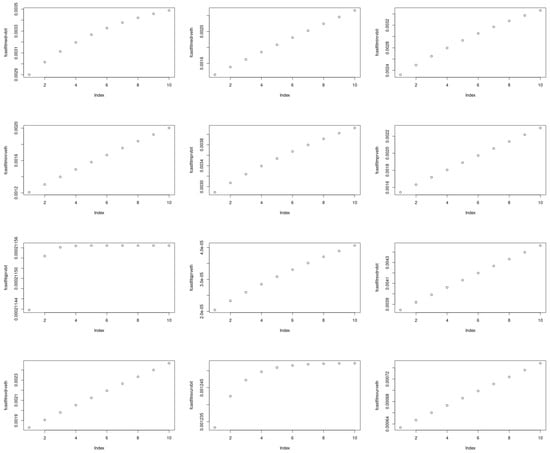
Figure 11.
Ten-day-ahead forecast for REGARCH-MIDAS-X models with jump-robust estimators (as the input) and volatility indices (as X).
6. Conclusions
A rich literature has now developed on Bitcoin, considered as a derivatives instrument. Following the methodology by Hasbrouck [66], Baur and Dimpfl [67] analyzed the trading volume and trading hours of the globally distributed Bitcoin spot market, compared to that of the U.S.-based CBOE/CME futures contracts introduced in December 2017. Entrop et al. [68] assessed that medium-sized trades, as well as news-based Bitcoin sentiment contain the most information in terms of price discovery on spot and futures markets. Alexander et al. [23] examined the price discovery and hedging effectiveness on the unregulated derivatives exchange BitMEX. Using minute-by-minute data, the authors demonstrated that BitMEX derivatives led prices on major Bitcoin spot exchanges, by looking primarily at inter-exchange spreads and relative trading volumes.
However, there is little literature on how financial variables could forecast the future movement of Bitcoin futures volatility. Moreover, there is virtually no contribution to how blockchain variables might affect Bitcoin’s price path. The literature on Ethereum is even more scarce on these latter topics. This paper proposed to fill these research gaps. We believe we are the first paper dealing with jump-robust high-frequency time series of Bitcoin and Ethereum augmented with hashrates (as the MIDAS filter) and volatility indices (as the exogenous variables). To do so, it appeared attractive to mobilize the research methodology for the REGARCH-MIDAS-X model, which provided an excellent framework for the joint modeling of returns and realized volatility measures.
With an original application to Bitcoin and Ethereum, the REGARCH-MIDAS-X model helped us analyze the link between financial volatility and the digital environment. The unit variance GARCH fluctuated around a time-varying long-term component, which is a function of each cryptocurrency’s hashrate. This MIDAS approach bridged the gap between high- (e.g., jump-robust intraday or daily) and low- (e.g., monthly) frequency data. The model explicitly distinguished short- and long-run Bitcoin and Ethereum volatility sources. Besides, the model enabled the inclusion of brokers’ volatility indices as exogenous variables (the ‘X’ factor) and linked them directly to blockchain in bivariate specifications. Last, but not least, we identified the realized GARCH as a very attractive model to be coupled with MIDAS filters, to capture volatility persistence better than the GARCH framework, and to deliver superior predictive ability (especially at shorter horizons).
Our results expose new essential findings on the Bitcoin and Ethereum market dynamics from May 2018 to January 2023. According to our experiments, the best ‘X’ factor to model Bitcoin and Ethereum’s high-frequency jump-robust returns stemmed from the 30-day implied volatility. Brokers such Triple3 Partners or Deribit can provide such an index. Regarding the MIDAS filtering, each cryptocurrency’s hashrate allowed us to determine the long-term component. Besides, we investigated the predictive ability of the REGARCH-MIDAS-X model for Bitcoin and Ethereum returns. Models driven by the broker’s Deribit 30-day implied volatility (and, for Ethereum once, CVI Finance’s Aggregate Crypto Volatility Index) performed the best in the out-of-sample prediction at a 10-day horizon. This informational content gleaned from options prices has a guiding significance for market participants, policymakers, and risk managers.
Author Contributions
Conceptualization, J.C.; methodology, B.S. and J.C.; software, B.S. and J.C.; validation, J.C. and B.S.; formal analysis, J.C. and B.S.; investigation, J.C. and B.S.; resources, B.S. and J.C.; data curation, B.S. and J.C.; writing—original draft preparation, J.C. and B.S.; writing—review and editing, J.C. and B.S.; visualization, B.S. All authors have read and agreed to the published version of the manuscript.
Funding
This research received no external funding.
Institutional Review Board Statement
Not applicable.
Informed Consent Statement
Not applicable.
Data Availability Statement
The monthly hashrate for Bitcoin was taken from https://data.nasdaq.com/data/BCHAIN/HRATE-bitcoin-hash-rate (accessed on 13 August 2023). Ethereum’s hashrate was sourced from https://etherscan.io/chart/hashrate?output=csv (accessed on 13 August 2023). The tick data for Bitcoin and Ethereum were sourced from https://www.cryptodatadownload.com/data/bitfinex/ (accessed on 13 August 2023). The Bitcoin Volatility Index (BVIN) is accessible at: https://www.cryptocompare.com/indices/bvin/ (accessed on 13 August 2023). The Crypto Volatility Index (CVI) is accessible at https://www.investing.com/indices/crypto-volatility-index-historical-data (accessed on 13 August 2023). Deribit’s DvolETH is located at https://metrics.deribit.com/options/ETH (accessed on 13 August 2023) and DvolBtc at https://metrics.deribit.com/options/BTC (accessed on 13 August 2023). Bitcoinity’s Bitcoin Price Volatility Index can be found at https://data.bitcoinity.org/markets/volatility/all/USD/bitfinex?f=m10&g=15&st=log&t=l (accessed on 13 August 2023). Compass FT’s Bitcoin Volatility Target 20% can be found at https://www.compassft.com/indice/cvtbtc20/ (accessed on 13 August 2023) and Ethereum Volatility Target 20% at https://www.compassft.com/indice/cvteth20/ (accessed on 13 August 2023). T3 Partners’ Indices BitVol and EthVol are both accessible at https://t3index.com/indexes/bit-vol/ (accessed on 13 August 2023). Volmex Finance’s ETHV historical data can be found at https://www.coingecko.com/en/coins/ethereum-volatility-index-token (accessed on 13 August 2023).
Conflicts of Interest
The authors declare no conflict of interest.
Appendix A
Appendix A.1. Descriptive Statistics of Bitcoin and Ethereum Jump-Robust Estimators

Table A1.
Descriptive statistics of Bitcoin and Ethereum jump-robust estimators.
Table A1.
Descriptive statistics of Bitcoin and Ethereum jump-robust estimators.
| Mean | Median | Min | Max | Std. Dev. | Skewness | Kurtosis | |
|---|---|---|---|---|---|---|---|
| rmedrvarbit | 0.0018 | 0.00094 | 0.000027 | 0.10 | 0.0037 | 13.52 | 305.62 |
| rminrvarbit | 0.0017 | 0.00087 | 0.000017 | 0.11 | 0.0038 | 15.30 | 366.82 |
| rmpvarbit | 0.0019 | 0.00100 | 0.000017 | 0.11 | 0.0040 | 14.71 | 342.10 |
| rqpvarbit | 0.0000 | 0.00000 | 0.000000 | 0.03 | 0.0007 | 39.15 | 1573.40 |
| rsvardownbit | 0.0012 | 0.00051 | 0.000009 | 0.09 | 0.0031 | 16.45 | 396.62 |
| rsvarupbit | 0.0011 | 0.00054 | 0.000008 | 0.06 | 0.0021 | 13.05 | 298.42 |
| rmedrvareth | 0.0010 | 0.00049 | 0.000007 | 0.07 | 0.0025 | 15.78 | 377.58 |
| rminrvareth | 0.0010 | 0.00046 | 0.000007 | 0.06 | 0.0023 | 13.72 | 292.88 |
| rmpvaeth | 0.0011 | 0.00054 | 0.000007 | 0.07 | 0.0025 | 15.48 | 376.64 |
| rqpvareth | 0.0000 | 0.00000 | 0.000000 | 0.01 | 0.0002 | 39.98 | 1628.50 |
| rsvardowneth | 0.0007 | 0.00028 | 0.000002 | 0.07 | 0.0022 | 21.83 | 656.12 |
| rsvarupeth | 0.0007 | 0.00029 | 0.000002 | 0.05 | 0.0017 | 16.55 | 426.54 |
Note: For Bitcoin, rmedrvarbit is the Median Realized Volatility estimator, rminrvarbit is the Minimum Variance Estimator, rmpvarbit the Realized MultiPower Estimator, rqpvarbit the Realized QuadPower Estimator, rsvardownbit the Realized Downside Semi-Variance Estimator, and rsvarupbit the Realized Upside Semi-Variance Estimator. Corresponding estimators are indexed by eth for Ethereum. The number of observations is equal to 1709.
Appendix A.2. Blockchain.com’s View of Bitcoin Price against the Hashrate

Figure A1.
Blockchain.com’s snapshot of Bitcoin’s price in USD against total hashrate from February 2009 until the present.
Figure A1.
Blockchain.com’s snapshot of Bitcoin’s price in USD against total hashrate from February 2009 until the present.
Appendix A.3. Descriptive Statistics of Bitcoin and Ethereum Volatility Indices

Table A2.
Descriptive statistics of Bitcoin and Ethereum volatility indices.
Table A2.
Descriptive statistics of Bitcoin and Ethereum volatility indices.
| Mean | Median | Min | Max | Std. Dev. | Skew. | Kurt. | Obs. | |
|---|---|---|---|---|---|---|---|---|
| BVIN | 84.29 | 83.75 | 39.13 | 174.29 | 21.57 | 0.63 | 0.82 | 1021 |
| CVI | 81.67 | 80.03 | 37.76 | 170.55 | 20.50 | 0.75 | 0.98 | 1579 |
| BitVol | 79.61 | 77.00 | 40.47 | 190.28 | 20.94 | 1.03 | 1.80 | 1490 |
| EthVol | 92.98 | 91.83 | 38.59 | 217.99 | 28.23 | 0.93 | 1.82 | 1187 |
| BTCDVOL | 39.71 | 39.27 | 34.15 | 46.43 | 3.06 | 0.08 | 471 | |
| ETHDVOL | 39.47 | 38.65 | 33.40 | 48.33 | 3.75 | 0.22 | 471 | |
| CVTBTC20 | 484.24 | 434.08 | 93.50 | 962.45 | 246.37 | 0.19 | 2761 | |
| CVTETH20 | 434.11 | 342.54 | 99.62 | 890.45 | 230.94 | 0.43 | 2761 | |
| Bitcoinity | 31.29 | 10.81 | 0.06 | 552.66 | 50.31 | 2.78 | 11.36 | 3789 |
| ETHV | 109.64 | 108.69 | 88.44 | 141.15 | 7.82 | 1.45 | 2.01 | 728 |
Note: BVIN is the Bitcoin Volatility Index, CVI the Crypto Volatility Index, BitVol T3 Partners’ Implied Volatility Index for Bitcoin, EthVol T3 Partners’ Implied Volatility Index for Ethereum, BTCDVOL Deribit’s Implied Volatility Index for Bitcoin, ETHDVOL Deribit’s Implied Volatility Index for Ethereum, CVTBTC20 Compass FT’s Bitcoin Historical Volatility Target 20% for Bitcoin, CVTETH20 Compass FT’s Bitcoin Historical Volatility Target 20% for Ethereum, Bitcoinity the historical standard deviation for Bitcoin calculated from Bitfinex, and ETHV Volmex Labs Finance’s Index of Ethereum Volatility. Std. Dev. stands for Standard Deviation, Kurt. for excess Kurtosis, Skew. for Skewness, and Obs. for the number of Observations.
Appendix A.4. Cyclic/Trend Decomposition and Simple Moving Average Channels for Bitcoin and Ethereum
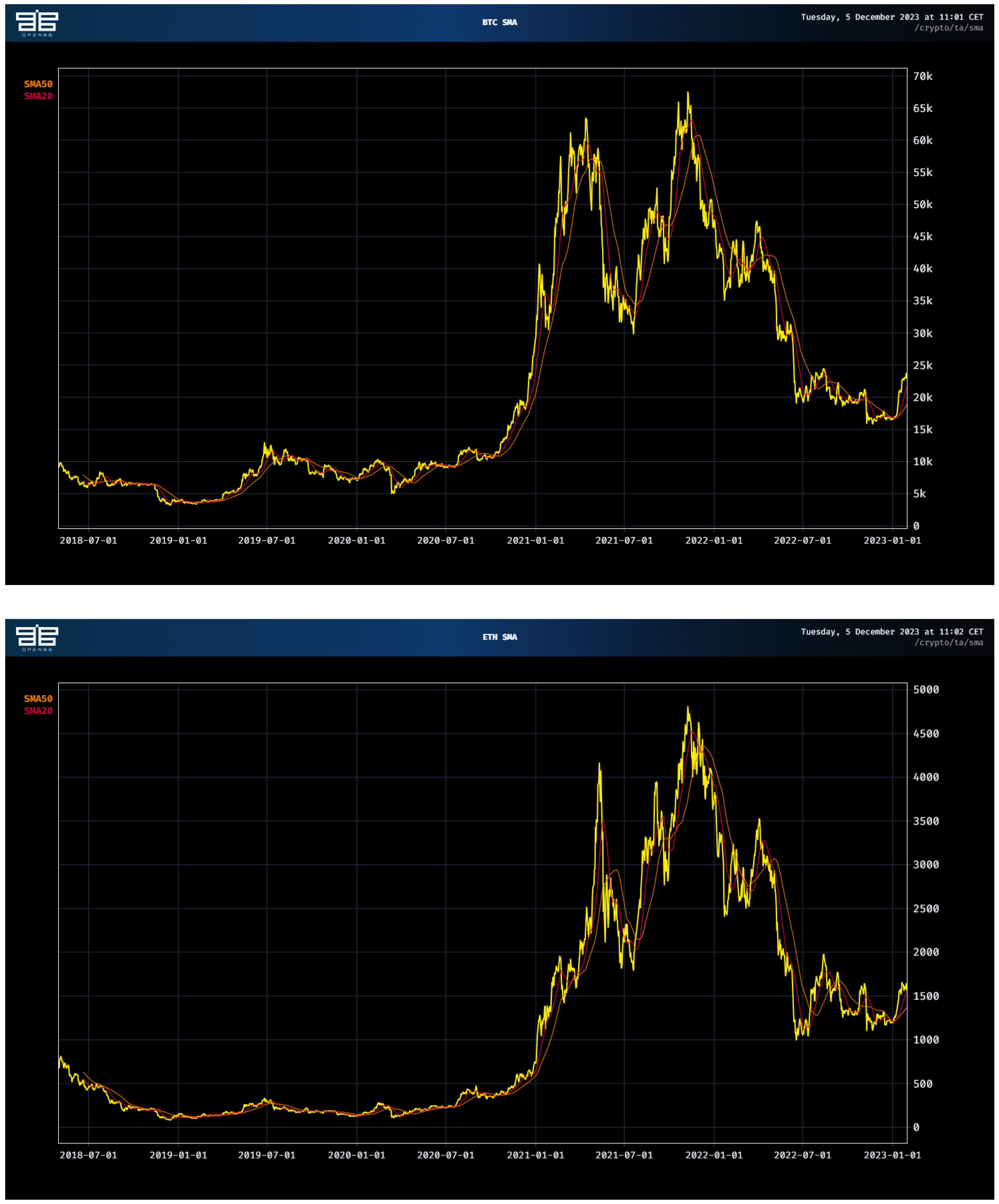
The sample considered was between May 2018 and January 2023. To analyze the long-memory behavior of the time series, we produced two graphs. One handles the decomposition of BTC and ETH into seasonal, trend, and cyclic components. The other reproduces a Simple Moving Average channel for BTC and ETH. The interested reader may glean from Figure A2 and Figure A3 that dramatic changes have impacted Bitcoin and Ethereum during the period January 2021–July 2022 especially, substantially inflating the prices before they dropped into what is known as the ‘crypto winter’.
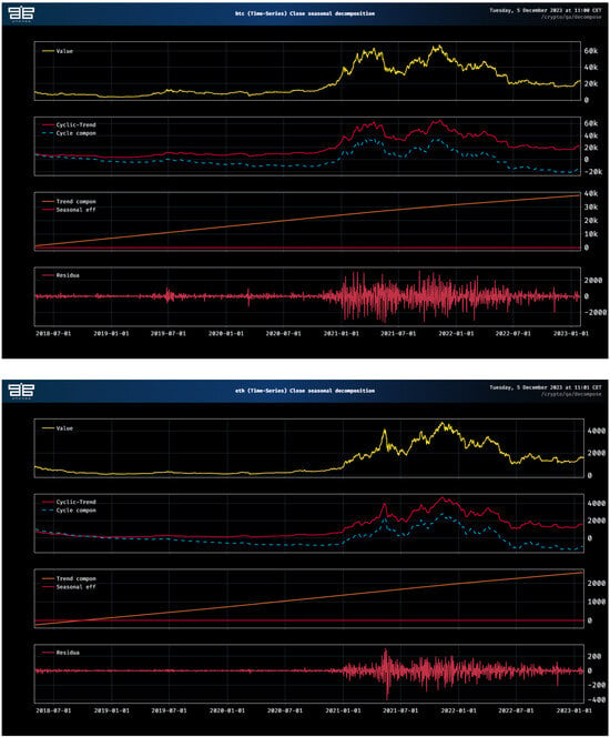
Figure A2.
Cyclic/trend decomposition for BTCUSD (top) and ETHUSD (bottom).
Figure A2.
Cyclic/trend decomposition for BTCUSD (top) and ETHUSD (bottom).
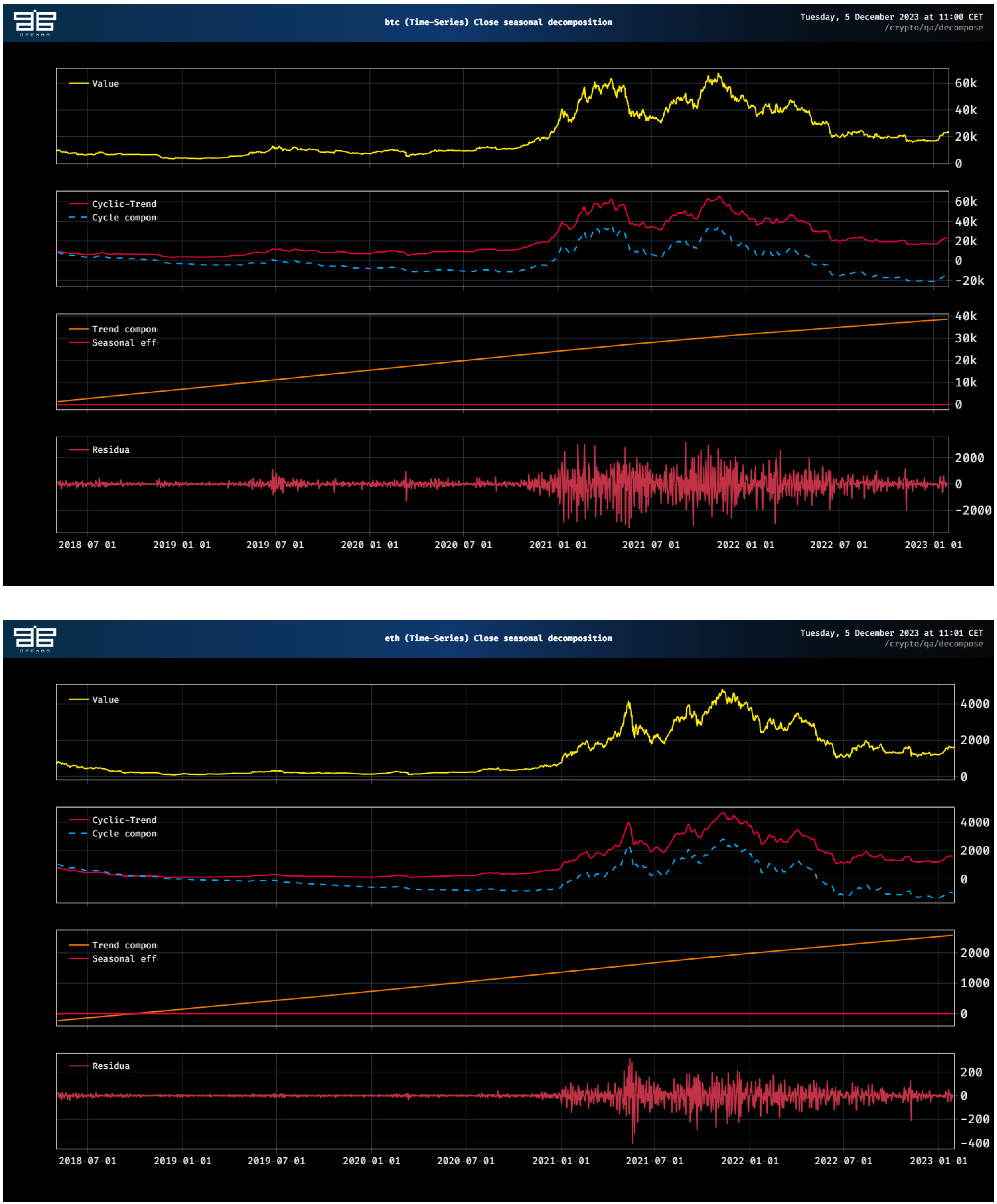
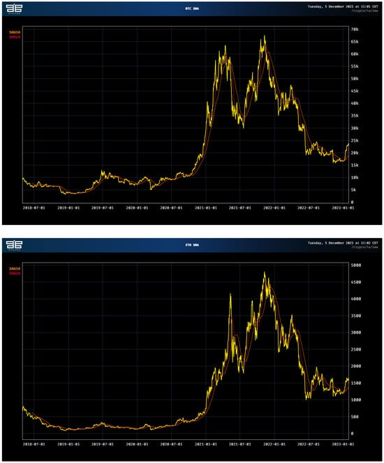
Figure A3.
SMA decomposition for BTCUSD (top) and ETHUSD (bottom).
Figure A3.
SMA decomposition for BTCUSD (top) and ETHUSD (bottom).
References
- Amendola, A.; Candila, V.; Gallo, G.M. Choosing the frequency of volatility components within the Double Asymmetric GARCH–MIDAS–X model. Econom. Stat. 2021, 20, 12–28. [Google Scholar] [CrossRef]
- Engle, R.F.; Ghysels, E.; Sohn, B. Stock market volatility and macroeconomic fundamentals. Rev. Econ. Stat. 2013, 95, 776–797. [Google Scholar] [CrossRef]
- Hansen, P.R.; Huang, Z.; Shek, H.H. Realized GARCH: A joint model for returns and realized measures of volatility. J. Appl. Econom. 2012, 27, 877–906. [Google Scholar] [CrossRef]
- Watanabe, T. Quantile forecasts of financial returns using realized GARCH models. Jpn. Econ. Rev. 2012, 63, 68–80. [Google Scholar] [CrossRef][Green Version]
- Tian, S.; Hamori, S. Modeling interest rate volatility: A realized GARCH approach. J. Bank. Financ. 2015, 61, 158–171. [Google Scholar] [CrossRef]
- Contino, C.; Gerlach, R.H. Bayesian tail-risk forecasting using realized GARCH. Appl. Stoch. Model. Bus. Ind. 2017, 33, 213–236. [Google Scholar] [CrossRef]
- Bonato, M. Realized correlations, betas and volatility spillover in the agricultural commodity market: What has changed? J. Int. Financ. Mark. Inst. Money 2019, 62, 184–202. [Google Scholar] [CrossRef]
- Borup, D.; Jakobsen, J.S. Capturing volatility persistence: A dynamically complete realized EGARCH-MIDAS model. Quant. Financ. 2019, 19, 1839–1855. [Google Scholar] [CrossRef]
- Wu, X.; Xie, H. A realized EGARCH-MIDAS model with higher moments. Financ. Res. Lett. 2021, 38, 101392. [Google Scholar] [CrossRef]
- Wu, X.; Wang, X.; Wang, H. Forecasting stock market volatility using implied volatility: Evidence from extended realized EGARCH-MIDAS model. Appl. Econ. Lett. 2021, 28, 915–920. [Google Scholar] [CrossRef]
- Wu, X.; He, Q.; Xie, H. Forecasting VIX with time-varying risk aversion. Int. Rev. Econ. Financ. 2023, 88, 458–475. [Google Scholar] [CrossRef]
- Wang, L.; Zhao, C.; Liang, C.; Jiu, S. Predicting the volatility of China’s new energy stock market: Deep insight from the realized EGARCH-MIDAS model. Financ. Res. Lett. 2022, 48, 102981. [Google Scholar] [CrossRef]
- Lu, X.; Su, Y.; Huang, D. Chinese agricultural futures volatility: New insights from potential domestic and global predictors. Int. Rev. Financ. Anal. 2023, 89, 102786. [Google Scholar] [CrossRef]
- Hung, J.C.; Liu, H.C.; Yang, J.J. Improving the realized GARCH’s volatility forecast for Bitcoin with jump-robust estimators. N. Am. J. Econ. Financ. 2020, 52, 101165. [Google Scholar] [CrossRef]
- Čuljak, M.; Arnerić, J.; Žigman, A. Is Jump Robust Two Times Scaled Estimator Superior among Realized Volatility Competitors? Mathematics 2022, 10, 2124. [Google Scholar] [CrossRef]
- Andersen, T.G.; Bollerslev, T.; Diebold, F.X. Roughing it up: Including jump components in the measurement, modeling, and forecasting of return volatility. Rev. Econ. Stat. 2007, 89, 701–720. [Google Scholar] [CrossRef]
- Caporin, M. The role of jumps in realized volatility modeling and forecasting. J. Financ. Econom. 2022, 21, nbab030. [Google Scholar] [CrossRef]
- Sanhaji, B.; Chevallier, J. Tracking ‘Pure’ Systematic Risk with Realized Betas for Bitcoin and Ethereum. Econometrics 2023, 11, 19. [Google Scholar] [CrossRef]
- Chen, X.; Ghysels, E.; Wang, F. HYBRID GARCH models and intra-daily return periodicity. J. Time Ser. Econom. 2011, 3, 1–38. [Google Scholar] [CrossRef]
- Chen, X.; Ghysels, E.; Wang, F. Hybrid-garch: A generic class of models for volatility predictions using high frequency data. Stat. Sin. 2015, 25, 759–786. [Google Scholar] [CrossRef]
- Adrian, T.; Rosenberg, J. Stock returns and volatility: Pricing the short-run and long-run components of market risk. J. Financ. 2008, 63, 2997–3030. [Google Scholar] [CrossRef]
- Calvet, L.E.; Fisher, A.J. Multifrequency news and stock returns. J. Financ. Econ. 2007, 86, 178–212. [Google Scholar] [CrossRef]
- Alexander, C.; Choi, J.; Park, H.; Sohn, S. BitMEX bitcoin derivatives: Price discovery, informational efficiency, and hedging effectiveness. J. Futures Mark. 2020, 40, 23–43. [Google Scholar] [CrossRef]
- Alexander, C.; Dakos, M. A critical investigation of cryptocurrency data and analysis. Quant. Financ. 2020, 20, 173–188. [Google Scholar] [CrossRef]
- Alexander, C.; Heck, D.F. Price discovery in Bitcoin: The impact of unregulated markets. J. Financ. Stab. 2020, 50, 100776. [Google Scholar] [CrossRef]
- Martens, M. Measuring and forecasting S&P 500 index-futures volatility using high-frequency data. J. Futur. Mark. Futur. Options Other Deriv. Prod. 2002, 22, 497–518. [Google Scholar]
- Huang, S.; Liu, Q.; Jun, Y. Realized daily variance of S&P 500 cash index: A revaluation of stylized facts. Ann. Econ. Financ. 2007, 8, 33. [Google Scholar]
- Andersen, T.G.; Dobrev, D.; Schaumburg, E. Jump-robust volatility estimation using nearest neighbor truncation. J. Econom. 2012, 169, 75–93. [Google Scholar] [CrossRef]
- Barndorff-Nielsen, O.E.; Kinnebrock, S.; Shephard, N. Measuring Downside Risk-Realised Semivariance; CREATES Research Paper; SSRN: Amsterdam, The Netherlands, 2008. [Google Scholar]
- Bollerslev, T.; Li, S.Z.; Zhao, B. Good volatility, bad volatility, and the cross section of stock returns. J. Financ. Quant. Anal. 2020, 55, 751–781. [Google Scholar] [CrossRef]
- Engle, R.F. Autoregressive conditional heteroscedasticity with estimates of the variance of United Kingdom inflation. Econom. J. Econom. Soc. 1982, 50, 987–1007. [Google Scholar] [CrossRef]
- Bollerslev, T. Generalized autoregressive conditional heteroskedasticity. J. Econom. 1986, 31, 307–327. [Google Scholar] [CrossRef]
- Andersen, T.G.; Bollerslev, T.; Diebold, F.X.; Labys, P. Modeling and forecasting realized volatility. Econometrica 2003, 71, 579–625. [Google Scholar] [CrossRef]
- Black, F. Capital market equilibrium with restricted borrowing. J. Bus. 1972, 45, 444–455. [Google Scholar] [CrossRef]
- Kuester, K.; Mittnik, S.; Paolella, M.S. Value-at-risk prediction: A comparison of alternative strategies. J. Financ. Econom. 2006, 4, 53–89. [Google Scholar] [CrossRef]
- Merton, R.C. On Estimating the Expected Return on the Market: An Exploratory Investigation; Technical Report; National Bureau of Economic Research: Cambridge, MA, USA, 1980. [Google Scholar]
- Schwert, G.W. Why does stock market volatility change over time? J. Financ. 1989, 44, 1115–1153. [Google Scholar] [CrossRef]
- Ghysels, E.; Sinko, A.; Valkanov, R. MIDAS regressions: Further results and new directions. Econom. Rev. 2007, 26, 53–90. [Google Scholar] [CrossRef]
- Hansen, P.R.; Lunde, A. Realized variance and market microstructure noise. J. Bus. Econ. Stat. 2006, 24, 127–161. [Google Scholar] [CrossRef]
- Hansen, P.R.; Lunde, A.; Voev, V. Realized beta GARCH: A multivariate GARCH model with realized measures of volatility. J. Appl. Econom. 2014, 29, 774–799. [Google Scholar] [CrossRef]
- Wang, F.; Ghysels, E. Econometric analysis of volatility component models. Econom. Theory 2015, 31, 362–393. [Google Scholar] [CrossRef]
- Hansen, P.R.; Huang, Z. Exponential GARCH modeling with realized measures of volatility. J. Bus. Econ. Stat. 2016, 34, 269–287. [Google Scholar] [CrossRef]
- Straumann, D.; Mikosch, T. Quasi-maximum-likelihood estimation in conditionally heteroscedastic time series: A stochastic recurrence equations approach. Ann. Stat. 2006, 34, 2449–2495. [Google Scholar] [CrossRef]
- Jensen, S.T.; Rahbek, A. Asymptotic inference for nonstationary GARCH. Econom. Theory 2004, 20, 1203–1226. [Google Scholar] [CrossRef]
- Jensen, S.T.; Rahbek, A. Asymptotic normality of the QMLE estimator of ARCH in the nonstationary case. Econometrica 2004, 72, 641–646. [Google Scholar] [CrossRef]
- Han, H.; Kristensen, D. Asymptotic theory for the QMLE in GARCH-X models with stationary and nonstationary covariates. J. Bus. Econ. Stat. 2014, 32, 416–429. [Google Scholar] [CrossRef]
- Han, H. Asymptotic properties of GARCH-X processes. J. Financ. Econom. 2015, 13, 188–221. [Google Scholar] [CrossRef]
- Francq, C.; Thieu, L.Q. Qml Inference For Volatility Models With Covariates. Econom. Theory 2019, 35, 37–72. [Google Scholar] [CrossRef]
- Paparoditis, E.; Politis, D.N. Resampling and subsampling for financial time series. In Handbook of Financial Time Series; Springer: Cham, Switzerland, 2009; pp. 983–999. [Google Scholar]
- Ghysels, E.; Santa-Clara, P.; Valkanov, R. The MIDAS Touch: Mixed Data Sampling Regression Models; Working Paper; University of North Carolina at Chapel Hill: Chapel Hill, NC, USA, 2004. [Google Scholar]
- Ghysels, E.; Santa-Clara, P.; Valkanov, R. There is a risk-return trade-off after all. J. Financ. Econ. 2005, 76, 509–548. [Google Scholar] [CrossRef]
- Ghysels, E.; Santa-Clara, P.; Valkanov, R. Predicting volatility: Getting the most out of return data sampled at different frequencies. J. Econom. 2006, 131, 59–95. [Google Scholar] [CrossRef]
- Katsiampa, P. Volatility estimation for Bitcoin: A comparison of GARCH models. Econ. Lett. 2017, 158, 3–6. [Google Scholar] [CrossRef]
- Conrad, C.; Loch, K. Anticipating long-term stock market volatility. J. Appl. Econom. 2015, 30, 1090–1114. [Google Scholar] [CrossRef]
- Fantazzini, D.; Kolodin, N. Does the hashrate affect the bitcoin price? J. Risk Financ. Manag. 2020, 13, 263. [Google Scholar] [CrossRef]
- Marthinsen, J.E.; Gordon, S.R. The price and cost of bitcoin. Q. Rev. Econ. Financ. 2022, 85, 280–288. [Google Scholar] [CrossRef]
- Kubal, J.; Kristoufek, L. Exploring the relationship between Bitcoin price and network’s hashrate within endogenous system. Int. Rev. Financ. Anal. 2022, 84, 102375. [Google Scholar] [CrossRef]
- Alexander, C.; Imeraj, A. The Bitcoin VIX and its variance risk premium. J. Altern. Invest. 2021, 23, 84–109. [Google Scholar] [CrossRef]
- Kim, A.; Trimborn, S.; Härdle, W.K. VCRIX—A volatility index for crypto-currencies. Int. Rev. Financ. Anal. 2021, 78, 101915. [Google Scholar] [CrossRef]
- Engle, R.F.; Rangel, J.G. The spline-GARCH model for low-frequency volatility and its global macroeconomic causes. Rev. Financ. Stud. 2008, 21, 1187–1222. [Google Scholar] [CrossRef]
- Conrad, C.; Kleen, O. Two are better than one: Volatility forecasting using multiplicative component GARCH-MIDAS models. J. Appl. Econom. 2020, 35, 19–45. [Google Scholar] [CrossRef]
- Ding, Z.; Granger, C.W. Modeling volatility persistence of speculative returns: A new approach. J. Econom. 1996, 73, 185–215. [Google Scholar] [CrossRef]
- Engle, R.F.; Lee, G. A long-run and short-run component model of stock return volatility. In Cointegration, Causality, and Forecasting: A Festschrift in Honour of Clive WJ Granger; Oxford University Press: Oxford, UK, 1999; pp. 475–497. [Google Scholar]
- Bandi, F.M.; Russell, J.R. Microstructure noise, realized variance, and optimal sampling. Rev. Econ. Stud. 2008, 75, 339–369. [Google Scholar] [CrossRef]
- Patton, A.J. Volatility forecast comparison using imperfect volatility proxies. J. Econom. 2011, 160, 246–256. [Google Scholar] [CrossRef]
- Hasbrouck, J. One security, many markets: Determining the contributions to price discovery. J. Financ. 1995, 50, 1175–1199. [Google Scholar] [CrossRef]
- Baur, D.G.; Dimpfl, T. Price discovery in bitcoin spot or futures? J. Futur. Mark. 2019, 39, 803–817. [Google Scholar] [CrossRef]
- Entrop, O.; Frijns, B.; Seruset, M. The Determinants of Price Discovery on Bitcoin Markets. J. Futures Mark. 2020, 40, 816–837. [Google Scholar] [CrossRef]
Disclaimer/Publisher’s Note: The statements, opinions and data contained in all publications are solely those of the individual author(s) and contributor(s) and not of MDPI and/or the editor(s). MDPI and/or the editor(s) disclaim responsibility for any injury to people or property resulting from any ideas, methods, instructions or products referred to in the content. |
© 2023 by the authors. Licensee MDPI, Basel, Switzerland. This article is an open access article distributed under the terms and conditions of the Creative Commons Attribution (CC BY) license (https://creativecommons.org/licenses/by/4.0/).

