The New Exponentiated Half Logistic-Harris-G Family of Distributions with Actuarial Measures and Applications

Abstract

In this study, we introduce a new generalized family of distributions called the Exponentiated Half Logistic-Harris-G (EHL-Harris-G) distribution, which extends the Harris-G distribution. The motivation for introducing this generalized family of distributions lies in its ability to overcome the limitations of previous families, enhance flexibility, improve tail behavior, provide better statistical properties and find applications in several fields. Several statistical properties, including hazard rate function, quantile function, moments, moments of residual life, distribution of the order statistics and Rényi entropy are discussed. Risk measures, such as value at risk, tail value at risk, tail variance and tail variance premium, are also derived and studied. To estimate the parameters of the EHL-Harris-G family of distributions, the following six different estimation approaches are used: maximum likelihood (MLE), least-squares (LS), weighted least-squares (WLS), maximum product spacing (MPS), Cramér–von Mises (CVM), and Anderson–Darling (AD). The Monte Carlo simulation results for EHL-Harris-Weibull (EHL-Harris-W) show that the MLE method allows us to obtain better estimates, followed by WLS and then AD. Finally, we show that the EHL-Harris-W distribution is superior to some other equi-parameter non-nested models in the literature, by fitting it to two real-life data sets from different disciplines.

1. Introduction

As distribution theory develops, it addresses the challenges researchers face, proposing a variety of models for better analyzing and exploring lifetime data sets. Consequently, useful models are necessary to better understand real phenomena in nature. Current trends and practices in constructing new probability models differ greatly from those proposed before 1997. A key objective of developing, extending, or generalizing models, and their classes, is to explain the lifetime phenomenon in a variety of fields, including physics, computer science, insurance, public health, medicine, engineering, biology, industry, communication, life testing, and so on.

Some well-known and fundamental distributions, such as Uniform, Beta, Exponential, Rayleigh, Weibull, and Gamma, do not demonstrate a wide range of flexibility. For example, the exponential distribution can be modeled with a constant hazard function, whereas the Rayleigh distribution can only be modeled with an increasing hazard function. The Weibull distribution, however, is more flexible and can be modeled with increasing, decreasing, or constant hazard functions. However, it cannot be used to model non-monotonic failure rate functions (such as unimodal or bathtub shapes), due to limitations in the Weibull distribution. It is difficult to describe the mathematical properties of the gamma distribution because there is no closed form of the cumulative distribution function. The failure rate behavior of complex phenomena, such as human mortality, reliability, lifetime testing, engineering modeling, electronic sciences, and biological surveys, may be bathtub-shaped, upside-down bathtub-shaped, and others, but is not usually monotonous. In response, researchers have developed several classes and families of generalized distributions for studying monotonic or non-monotonic failure rates in models.

Over the years, several new and very useful classes and families of distributions have been developed, as well as generalized distributions obtained by adding one or more parameters to existing distributions. As a result of the extra parameters introduced, the tail weight and entropy of a density function can be controlled, depending on the resulting distribution. Some of the well-known families, to mention just a few of these, are as follow: the Marshall-Olkin-G, by [1], the beta-G, by [2], the transmuted-G, by [3], the gamma-G, by [4], the Kumaraswamy-G, by [5], the exponentiated generalized-G by [6], the T-X family, by [7], the logistic-G, by [8], the Weibull-G, by [9], and the odd log-logistic-G by [10], the type II half logistic family of distributions, by [11], the odd log-logistic Topp–Leone G family of distributions, by [12], the type II half logistic Kumaraswamy distribution, by [13], the exponentiated half-logistic odd Lindley-G family of distributions, by [14], the type II kumaraswamy half logistic family of distributions, by [15], the half logistic log-logistic Weibull distribution, by [16], the half logistic modified Kies exponential distribution, by [17], a class of distributions which includes the normal ones by [18], the stable symmetric family of distributions, by [19], towards the establishment of a family of distributions that best fits any data set, by [20], and the generation of distribution functions, by [21].

The Exponentiated Half Logistic-G (EHL-G) family of distributions was developed by [22]. The cumulative distribution function (cdf) and probability density function (pdf) of the EHL-G family distributions is given by:

$$\begin{array}{ccc}\hfill F_{EHL-G}(x;\alpha ,\zeta )& =& {\left[\frac{1-{\overline{G}}^{\lambda }(x;\zeta )}{1+{\overline{G}}^{\lambda }(x;\zeta )}\right]}^{\alpha },\hfill \end{array}$$

(1)

and

$$\begin{array}{ccc}\hfill f_{EHL-G}(x;\alpha ,\zeta )& =& 2\alpha \lambda g(x;\zeta ){\left(1-G(x;\zeta )\right)}^{\lambda -1}\frac{{[1-{\overline{G}}^{\lambda }(x;\zeta )]}^{\alpha -1}}{{[1+{\overline{G}}^{\lambda }(x;\zeta )]}^{\alpha +1}},\hfill \end{array}$$

(2)

respectively, for $x>0$, $\alpha >0$ and parameter vector $\zeta$. Pinho et al. [23] developed the Harris-G class of distributions with the cdf and pdf given as:

$$\begin{array}{ccc}\hfill F_{H-G}(x;\theta ,v,\zeta )& =& 1-{\left[\frac{\theta {\overline{G}}^v(x;\zeta )}{1-\overline{\theta }{\overline{G}}^v(x;\zeta )}\right]}^{\frac{1}{v}}\hfill \end{array}$$

(3)

and

$$\begin{array}{ccc}\hfill f_{H-G}(x;\theta ,v,\zeta )& =& \frac{{\theta }^{\frac{1}{v}}g(x;\zeta )}{{\left[1-\overline{\theta }{\overline{G}}^v(x;\zeta )\right]}^{1+\frac{1}{v}}},\hfill \end{array}$$

(4)

for $\theta ,v>0,\overline{\theta }=1-\theta ,$ and parameter vector $\zeta$, respectively. In this study, we introduce a new generalized family of distributions called the Exponentiated Half Logistic-Harris-G (EHL-Harris-G) distribution, which extends the Harris-G distribution by  [23].

An empirical study on loss distributions was carried out by [24], using exploratory data analysis and empirical methods to estimate risk. They ruled out the use of exponential, gamma, and Weibull distributions, due to their lack of flexibility and poor results, and said, “one would need to use a model that is flexible enough”. Therefore, it is essential to develop models based on existing distributions, or create new models that are applicable in the areas of financial risk management, insurance and actuarial sciences, climate science, extreme value analysis and portfolio optimization. In light of the premises outlined above, we were motivated to seek out more flexible probability distributions to provide greater accuracy in fitting data. Therefore, several factors motivated the development of the exponentiated half logistic-Harris-G (EHL-Harris-G) family of distributions: (i) its ability to overcome the limitations of previous distributions, enhance flexibility, improve tail behavior, provide better statistical properties, and find applications in several fields; (ii) to define special models with a good number of different shapes of hazard rate function; (iii) to produce skewness for symmetrical models; (iv) to provide consistently better fits than other generalized distributions with the same underlying model; (v) to generalize some existing models in the literature; (vi) to modulate the weight of the tails of any baseline distribution. The areas of applicability for the EHL-Harris-G family of distributions in research include financial risk management, insurance and actuarial sciences, climate science, extreme value analysis and portfolio optimization.

The rest of the work is organized in the following manner. Section 2 presents the novel exponentiated half-logistic-Harris-G (EHL-Harris-G) family of distributions, reliability and hazard rate function, sub-families, linear representation and quantile function. In Section 3, moments, moment generating function, moments of residual life, the distribution of order statistics, and Rényi entropy are presented. Section 4 contains six different estimation methods to estimate the unknown parameters of the EHL-Harris-G family of distributions. In Section 5, some special models from the EHL-Harris-G family of distributions are presented. In Section 6, Monte Carlo simulations are employed to examine the consistency property of six estimation methods for the EHL-Harris-G distribution family. In Section 7, actuarial measures and numerical studies of these measures are presented. Real data applications are given in Section 8, followed by some concluding remarks in Section 9.

2. The New Family of Distributions

In this section, we define the cdf and the pdf of the exponentiated Half Logistic-Harris-G (EHL-Harris-G) family of distributions by considering a case where $\lambda =1$ is in Equation (1). Then the pdf and the cdf of the Harris-G distribution, defined by (3) and (4), are substituted into Equations (1) and (2). The resulting cdf and pdf of the EHL-Harris-G family of distributions are, respectively, given by:

$$F(x;\alpha ,v,\delta ,\zeta )={\left[\frac{1-{\left(\frac{\delta {\overline{G}}^v(x;\zeta )}{1-\overline{\delta }{\overline{G}}^v(x;\zeta )}\right)}^{\frac{1}{v}}}{1+{\left(\frac{\delta {\overline{G}}^v(x;\zeta )}{1-\overline{\delta }{\overline{G}}^v(x;\zeta )}\right)}^{\frac{1}{v}}}\right]}^{\alpha },$$

(5)

and

$$\begin{array}{ccc}\hfill f(x;\alpha ,v,\delta ,\zeta )& =& 2\alpha {\delta }^{\frac{1}{v}}g(x;\zeta ){\left(1-\overline{\delta }{\overline{G}}^v(x;\zeta )\right)}^{-(\frac{1}{v}+1)}{\left[1-{\left(\frac{\delta {\overline{G}}^v(x;\zeta )}{1-\overline{\delta }{\overline{G}}^v(x;\zeta )}\right)}^{\frac{1}{v}}\right]}^{\alpha -1}\hfill \\ & \times & {\left[1+{\left(\frac{\delta {\overline{G}}^v(x;\zeta )}{1-\overline{\delta }{\overline{G}}^v(x;\zeta )}\right)}^{\frac{1}{v}}\right]}^{-(\alpha +1)},\hfill \end{array}$$

(6)

for $\alpha ,v,\delta >0$, $\overline{\delta }=1-\delta ,$ $x>0$ and parameter vector $\zeta$, where G is the baseline cdf.

2.1. Reliability Measures

The survival function and hazard rate function (hrf) of the EHL-Harris-G family of distributions are given by:

$$\begin{array}{c}\hfill S\left(x\right)=1-{\left[\frac{1-{\left(\frac{\delta {\overline{G}}^v(x;\zeta )}{1-\overline{\delta }{\overline{G}}^v(x;\zeta )}\right)}^{\frac{1}{v}}}{1+{\left(\frac{\delta {\overline{G}}^v(x;\zeta )}{1-\overline{\delta }{\overline{G}}^v(x;\zeta )}\right)}^{\frac{1}{v}}}\right]}^{\alpha },\end{array}$$

(7)

and

$$\begin{array}{ccc}\hfill h\left(x\right)& =& 2\alpha {\delta }^{\frac{1}{v}}g(x;\zeta ){\left(1-\overline{\delta }{\overline{G}}^v(x;\zeta )\right)}^{-(\frac{1}{v}+1)}{\left[1-{\left(\frac{\delta {\overline{G}}^v(x;\zeta )}{1-\overline{\delta }{\overline{G}}^v(x;\zeta )}\right)}^{\frac{1}{v}}\right]}^{\alpha -1}\hfill \\ & \times & {\left[1+{\left(\frac{\delta {\overline{G}}^v(x;\zeta )}{1-\overline{\delta }{\overline{G}}^v(x;\zeta )}\right)}^{\frac{1}{v}}\right]}^{-(\alpha +1)}{\left(1-{\left[\frac{1-{\left(\frac{\delta {\overline{G}}^v(x;\zeta )}{1-\overline{\delta }{\overline{G}}^v(x;\zeta )}\right)}^{\frac{1}{v}}}{1+{\left(\frac{\delta {\overline{G}}^v(x;\zeta )}{1-\overline{\delta }{\overline{G}}^v(x;\zeta )}\right)}^{\frac{1}{v}}}\right]}^{\alpha }\right)}^{-1},\hfill \end{array}$$

(8)

for $\alpha ,v,\delta >0$, $\overline{\delta }=1-\delta$ and parameter vector $\zeta$, respectively. The cumulative hazard rate function of the EHL-Harris-G family of distributions is given by:

$$\begin{array}{c}\hfill H\left(x\right)=-ln\left(S\left(x\right)\right)=-ln\left(1-{\left[\frac{1-{\left(\frac{\delta {\overline{G}}^v(x;\zeta )}{1-\overline{\delta }{\overline{G}}^v(x;\zeta )}\right)}^{\frac{1}{v}}}{1+{\left(\frac{\delta {\overline{G}}^v(x;\zeta )}{1-\overline{\delta }{\overline{G}}^v(x;\zeta )}\right)}^{\frac{1}{v}}}\right]}^{\alpha }\right).\end{array}$$

(9)

2.2. Sub-Families of EHL-Harris-G Family of Distributions

• When $v=1,$ we obtain the exponentiated half logistic-Marshall-Olkin-G family of distributions with the cdf:

  $$\begin{array}{c}\hfill F(x;\alpha ,\delta ,\zeta )={\left[\frac{1-\frac{\delta \overline{G}(x;\zeta )}{1-\overline{\delta }\overline{G}(x;\zeta )}}{1+\frac{\delta \overline{G}(x;\zeta )}{1-\overline{\delta }\overline{G}(x;\zeta )}}\right]}^{\alpha },\end{array}$$

  for $\alpha ,\delta >0$ and parameter vector $\zeta .$ This is a new family of distributions.
• When $\alpha =1,$ we obtain the half logistic-Harris-G family of distributions with the cdf:

  $$F(x;v,\delta ,\zeta )=\frac{1-{\left(\frac{\delta {\overline{G}}^v(x;\zeta )}{1-\overline{\delta }{\overline{G}}^v(x;\zeta )}\right)}^{\frac{1}{v}}}{1+{\left(\frac{\delta {\overline{G}}^v(x;\zeta )}{1-\overline{\delta }{\overline{G}}^v(x;\zeta )}\right)}^{\frac{1}{v}}},$$

  for $v,\delta >0$ and parameter vector $\zeta .$ This is a new family of distributions.
• When $\delta =1,$ we obtain a reduced EHL-G family of distributions with the cdf:

  $$F(x;\alpha ,\zeta )={\left[\frac{1-\overline{G}(x;\zeta )}{1+\overline{G}(x;\zeta )}\right]}^{\alpha }={\left[\frac{G(x;\zeta )}{1+\overline{G}(x;\zeta )}\right]}^{\alpha },$$

  for $\alpha >0,$ and parameter vector $\zeta .$ See [22] for details.
• When $\alpha =v=1,$ we obtain the half logistic-Marshall-Olkin-G (HL-MO-G) family of distributions new family of distributions with the cdf:

  $$F(x;\delta ,\zeta )=\frac{1-\left(\frac{\delta \overline{G}(x;\zeta )}{1-\overline{\delta }\overline{G}(x;\zeta )}\right)}{1+\left(\frac{\delta \overline{G}(x;\zeta )}{1-\overline{\delta }{\overline{G}}^v(x;\zeta )}\right)},$$

  for $\delta >0,$ and parameter vector $\zeta .$
• If $\alpha =\delta =1,$ we obtain a reduced Half Logistic-G (HL-G) family of distributions with the cdf:

  $$F(x;\zeta )=\frac{1-\overline{G}(x;\zeta )}{1+\overline{G}(x;\zeta )}=\frac{G(x;\zeta )}{1+\overline{G}(x;\zeta )},$$

  for parameter vector $\zeta .$ See [22] for additional details.
• If $v=\delta =1,$ we obtain a reduced EHL-G family of distributions with the cdf:

  $$F(x;\alpha ,\zeta )={\left[\frac{G(x;\zeta )}{1+\overline{G}(x;\zeta )}\right]}^{\alpha },$$

  for $\alpha >0$ and parameter vector $\zeta .$ See [22] for details.

2.3. Linear Representation

In this sub-section, we express the pdf of the EHL-Harris-G family of distributions as an infinite linear combination of exponentiated-G (Exp-G) densities. Making use of the following generalized series expansions,

$$\begin{array}{c}\hfill {(1-z)}^{-n}=\sum _{ı=0}^{\infty }{(-1)}^i\left(\genfrac{}{}{0pt}{}{n+i-1}{i}\right)z^i\mathrm{for}\left|z\right|<1,\end{array}$$

the pdf of the EHL-Harris-G family of distributions can be expressed as follows:

$$\begin{array}{ccc}\hfill f(x;\alpha ,v,\delta ,\zeta )& =& 2\alpha {\delta }^{\frac{1}{v}}g(x;\zeta ){\left(1-\overline{\delta }{\overline{G}}^v(x;\zeta )\right)}^{-(\frac{1}{v}+1)}{\left[1-{\left(\frac{\delta {\overline{G}}^v(x;\zeta )}{1-\overline{\delta }{\overline{G}}^v(x;\zeta )}\right)}^{\frac{1}{v}}\right]}^{\alpha -1}\hfill \\ & \times & {\left[1+{\left(\frac{\delta {\overline{G}}^v(x;\zeta )}{1-\overline{\delta }{\overline{G}}^v(x;\zeta )}\right)}^{\frac{1}{v}}\right]}^{-(\alpha +1)}\hfill \\ & =& 2\alpha g(x;\zeta )\sum _{m,n=0}^{\infty }{(-1)}^n{\delta }^{\frac{1}{v}(m+n+1)}\left(\genfrac{}{}{0pt}{}{\alpha +m}{m}\right)\left(\genfrac{}{}{0pt}{}{\alpha -1}{n}\right){\overline{G}}^{m+n}(x;\zeta )\hfill \\ & \times & {\left[1-\overline{\delta }{\overline{G}}^v(x;\zeta )\right]}^{-(\frac{1}{v}(m+n+1)+1)}\hfill \\ & =& 2\alpha g(x;\zeta )\sum _{m,n,k=0}^{\infty }{(-1)}^{n+k}{\delta }^{\frac{1}{v}(m+n+1)}{\overline{\delta }}^k\left(\genfrac{}{}{0pt}{}{\alpha +m}{m}\right)\left(\genfrac{}{}{0pt}{}{\frac{1}{v}(m+n+1)+k}{k}\right)\hfill \\ & \times & \left(\genfrac{}{}{0pt}{}{\alpha -1}{n}\right){\overline{G}}^{vk+m+n}(x;\zeta )\hfill \\ & =& 2\alpha g(x;\zeta )\sum _{m,n,k,p=0}^{\infty }{(-1)}^{n+k+p}{\delta }^{\frac{1}{v}(m+n+1)}{\overline{\delta }}^k\left(\genfrac{}{}{0pt}{}{\frac{1}{v}(m+n+1)+k}{k}\right)\hfill \\ & \times & \left(\genfrac{}{}{0pt}{}{\alpha +m}{m}\right)\left(\genfrac{}{}{0pt}{}{\alpha -1}{n}\right)\left(\genfrac{}{}{0pt}{}{vk+m+n}{p}\right)G^p(x;\zeta )\hfill \\ & =& \sum _{p=0}^{\infty }{\phi }_{p+1}{g}_{p+1}(x;\zeta ),\hfill \end{array}$$

(10)

where $g_{p+1}(x;\zeta )=(p+1){\left[G(x;\zeta )\right]}^{p}g(x;\zeta )$ is the Exp-G pdf with the power parameter $(p+1)$ and parameter vector $\zeta ,$ and

$$\begin{array}{ccc}\hfill {\phi }_{p+1}& =& 2\alpha \sum _{m,n,k,p=0}^{\infty }\frac{{(-1)}^{n+k+p}{\delta }^{\frac{1}{v}(m+n+1)}{\overline{\delta }}^k}{p+1}\left(\genfrac{}{}{0pt}{}{\frac{1}{v}(m+n+1)+k}{k}\right)\hfill \\ & \times & \left(\genfrac{}{}{0pt}{}{\alpha +m}{m}\right)\left(\genfrac{}{}{0pt}{}{\alpha -1}{n}\right)\left(\genfrac{}{}{0pt}{}{vk+m+n}{p}\right).\hfill \end{array}$$

(11)

Thus, the statistical properties of the EHL-Harris-G family of distributions can be obtained from those of the Exp-G family of distributions.

2.4. Quantile Function

The quantile function is a very useful quantity in many statistical applications and Monte-Carlo methods. It is used to generate some random numbers from a distribution and is obtained by the inverting pf the cdf of a distribution. Let us assume X to be a random variable following the EHL-Harris-G family of distributions. Then, the quantile function of X can be obtained as follows:

$$F(x;\alpha ,v,\delta ,\zeta )={\left[\frac{1-{\left(\frac{\delta {\overline{G}}^v(x;\zeta )}{1-\overline{\delta }{\overline{G}}^v(x;\zeta )}\right)}^{\frac{1}{v}}}{1+{\left(\frac{\delta {\overline{G}}^v(x;\zeta )}{1-\overline{\delta }{\overline{G}}^v(x;\zeta )}\right)}^{\frac{1}{v}}}\right]}^{\alpha }=u,$$

(12)

for $0\le u\le 1$, that is,

$$G(x;\zeta )=1-{\left({\left[\frac{1-u^{\frac{1}{\alpha }}}{1+u^{\frac{1}{\alpha }}}\right]}^{-v}\delta +\overline{\delta }\right)}^{-\frac{1}{v}}.$$

(13)

Consequently, the quantile function of the EHL-Harris-G family of distributions is given by:

$$Q_X\left(u\right)=G^{-1}\left[1-{\left({\left[\frac{1-u^{\frac{1}{\alpha }}}{1+u^{\frac{1}{\alpha }}}\right]}^{-v}\delta +\overline{\delta }\right)}^{-\frac{1}{v}}\right].$$

(14)

Subsequently, using Equation (14) for the specified baseline cdf G, we can generate random variates from the EHL-Harris-G family of distributions for a specified baseline cdf G.

3. Statistical Properties

In this section, we provide some of the statistical properties of the EHL-Harris-G family of distributions, such as moments, the moment generating function, moments of residual life, distribution of order statistics and Rényi entropy. Throughout this section, we consider $f\left(x\right)=f(x;\alpha ,v,\delta ,\zeta )$ without any loss of generality to be the pdf of the EHL-Harris-G family of distributions.

3.1. Moments and Generating Function

Let $Y_{p+1}\sim Exponentiated-G(p+1,\zeta )$, then, the $r^{th}$ raw moment, ${\mu }_r^{\prime }$, of the EHL-Harris-G family of distributions is given by:

$${\mu }_r^{\prime }=E\left(X^r\right)={\int }_{-\infty }^{\infty }{x}^{r}f\left(x\right)dx=\sum _{p=0}^{\infty }{\phi }_{p+1}E\left(Y_{p+1}^r\right),$$

where $E\left(Y_{p+1}^r\right)$ is the $r^{th}$ moment of $Y_{p+1}$ and ${\phi }_{p+1}$ is given by Equation (11). The moment generating function (MGF), for $\left|t\right|<1$, is given by:

$$M_X\left(t\right)=E\left(e^{tX}\right)=\sum _{p=0}^{\infty }{\phi }_{p+1}{M}_{p+1}\left(t\right),$$

where $M_{p+1}\left(t\right)$ is the mgf of $Y_{p+1}$ and ${\phi }_{p+1}$ is given by Equation (11).

3.2. Order Statistics

In reliability theory and quality control testing, order statistics plays a vital role in predicting the time to failure of components. Suppose $X_1,X_2,\dots ,X_z$ are independent and identically distributed random variables from the EHL-Harris-G family of distributions. The pdf of the $i^{th}$ order statistic of X from the EHL-Harris-G pdf $f\left(x\right)$ can be written as

$$\begin{array}{ccc}\hfill f_{i:z}\left(x_{\left(i\right)}\right)& =& \frac{z!f\left(x_{\left(i\right)}\right)}{(i-1)!(z-i)!}\sum _{q=0}^{z-i}{(-1)}^q\left(\genfrac{}{}{0pt}{}{z-i}{q}\right){\left[F\left(x_{\left(i\right)}\right)\right]}^{q+i-1}.\hfill \end{array}$$

(15)

Using Equations (5) and (6), we have

$$\begin{array}{ccc}\hfill f\left(x_{\left(i\right)}\right){\left[F\left(x_{\left(i\right)}\right)\right]}^{q+i-1}& =& 2\alpha {\delta }^{\frac{1}{v}}g(x_{\left(i\right)};\zeta ){\left(1-\overline{\delta }{\overline{G}}^v(x_{\left(i\right)};\zeta )\right)}^{-(\frac{1}{v}+1)}\hfill \\ & \times & {\left[1-{\left(\frac{\delta {\overline{G}}^v(x_{\left(i\right)};\zeta )}{1-\overline{\delta }{\overline{G}}^v(x_{\left(i\right)};\zeta )}\right)}^{\frac{1}{v}}\right]}^{\alpha (q+i)-1}\hfill \\ & \times & {\left[1+{\left(\frac{\delta {\overline{G}}^v(x_{\left(i\right)};\zeta )}{1-\overline{\delta }{\overline{G}}^v(x_{\left(i\right)};\zeta )}\right)}^{\frac{1}{v}}\right]}^{-\left(\alpha \right(q+i)+1)}\hfill \\ & =& 2\alpha g(x_{\left(i\right)};\zeta )\sum _{m,n=0}^{\infty }{(-1)}^n{\delta }^{\frac{1}{v}(m+n+1)}\left(\genfrac{}{}{0pt}{}{\alpha (q+i)+m}{m}\right)\hfill \\ & \times & \left(\genfrac{}{}{0pt}{}{\alpha (q+i)-1}{n}\right){\overline{G}}^{m+n}(x_{\left(i\right)};\zeta ){(1-\overline{\delta }{\overline{G}}^v(x_{\left(i\right)};\zeta ))}^{-(\frac{1}{v}(m+n+1)+1)}\hfill \\ & =& 2\alpha g(x_{\left(i\right)};\zeta )\sum _{m,n,k,p=0}^{\infty }{(-1)}^{n+k+p}{\overline{\delta }}^k{\delta }^{\frac{1}{v}(m+n+1)}\left(\genfrac{}{}{0pt}{}{\alpha (q+i)+m}{m}\right)\hfill \\ & \times & \left(\genfrac{}{}{0pt}{}{\alpha (q+i)-1}{n}\right)\left(\genfrac{}{}{0pt}{}{\frac{1}{v}(m+n+1)+k}{k}\right)\left(\genfrac{}{}{0pt}{}{vk+m+n}{p}\right)G^p(x_{\left(i\right)};\zeta )\hfill \\ & =& \sum _{p=0}^{\infty }{\psi }_{p+1}{g}_{p+1}(x_{\left(i\right)};\zeta ),\hfill \end{array}$$

(16)

where $g_{p+1}(x_{\left(i\right)};\zeta )=(p+1){\left[G(x_{\left(i\right)};\zeta )\right]}^{p}g(x_{\left(i\right)};\zeta )$ is the Exp-G pdf with the power parameter $(p+1)$ and parameter vector $\zeta ,$ and

$$\begin{array}{ccc}\hfill {\psi }_{p+1}& =& 2\alpha \sum _{m,n,k,p=0}^{\infty }\frac{{(-1)}^{n+k+p}{\overline{\delta }}^k{\delta }^{\frac{1}{v}(m+n+1)}}{p+1}\left(\genfrac{}{}{0pt}{}{\alpha (q+i)+m}{m}\right)\hfill \\ & \times & \left(\genfrac{}{}{0pt}{}{\alpha (q+i)-1}{n}\right)\left(\genfrac{}{}{0pt}{}{\frac{1}{v}(m+n+1)+k}{k}\right)\left(\genfrac{}{}{0pt}{}{vk+m+n}{p}\right).\hfill \end{array}$$

(17)

Thus, by substituting (16) into (15), the pdf of the $i^{th}$ order statistic of X from the EHL-Harris-G family of distributions can be written as:

$$\begin{array}{ccc}\hfill f_{i:z}\left(x_{\left(i\right)}\right)& =& \frac{z!}{(i-1)!(z-i)!}\sum _{p=0}^{\infty }\sum _{q=0}^{z-i}{(-1)}^q\left(\genfrac{}{}{0pt}{}{z-i}{q}\right){\psi }_{p+1}{g}_{p+1}(x_{\left(i\right)};\zeta ).\hfill \end{array}$$

(18)

This shows that the pdf of $i^{th}$ order statistic of X from the EHL-Harris-G family of distributions can be obtained from those of the Exp-G family of distributions.

3.3. Rényi Entropy

Rényi entropy is a measure of randomness or uncertainty in the system. It is mostly used in information theory. Rényi entropy is defined as:

$$I_R\left(\theta \right)=\frac{1}{1-\theta }log\left({\int }_0^{\infty }{\left[f\left(x\right)\right]}^{\theta }dx\right),\theta \ne 1,\theta >0.$$

(19)

Note that

$$\begin{array}{ccc}\hfill {\left[f\left(x\right)\right]}^{\theta }& =& {\left(2\alpha \right)}^{\theta }{\delta }^{\frac{\theta }{v}}{g}^{\theta }(x;\zeta ){\left(1-\overline{\delta }{\overline{G}}^v(x;\zeta )\right)}^{-\theta (\frac{1}{v}+1)}\hfill \\ & \times & {\left[1-{\left(\frac{\delta {\overline{G}}^v(x;\zeta )}{1-\overline{\delta }{\overline{G}}^v(x;\zeta )}\right)}^{\frac{1}{v}}\right]}^{\theta (\alpha -1)}{\left[1+{\left(\frac{\delta {\overline{G}}^v(x;\zeta )}{1-\overline{\delta }{\overline{G}}^v(x;\zeta )}\right)}^{\frac{1}{v}}\right]}^{-\theta (\alpha +1)}\hfill \\ & =& {\left(2\alpha \right)}^{\theta }{g}^{\theta }(x;\zeta )\sum _{m,n,k,p=0}^{\infty }{(-1)}^{n+k+p}{\overline{\delta }}^k{\delta }^{\frac{1}{v}(m+n+\theta )}\left(\genfrac{}{}{0pt}{}{\theta (\alpha +1)+m-1}{m}\right)\hfill \\ & \times & \left(\genfrac{}{}{0pt}{}{\theta (\alpha -1)}{n}\right)\left(\genfrac{}{}{0pt}{}{\frac{1}{v}(m+n+\theta )+k-\theta -1}{k}\right)\left(\genfrac{}{}{0pt}{}{vk+m+n}{p}\right)G^p(x;\zeta ).\hfill \end{array}$$

Rényi entropy for the EHL-Harris-G family of distributions is given by:

$$\begin{array}{ccc}\hfill I_R\left(\theta \right)& =& \frac{1}{1-\theta }log[\sum _{m,n,k,p=0}^{\infty }{\left(2\alpha \right)}^{\theta }{(-1)}^{n+k+p}{\overline{\delta }}^k{\delta }^{\frac{1}{v}(m+n+\theta )}\left(\genfrac{}{}{0pt}{}{\theta (\alpha +1)+m-1}{m}\right)\hfill \\ & \times & \left(\genfrac{}{}{0pt}{}{\theta (\alpha -1)}{n}\right)\left(\genfrac{}{}{0pt}{}{\frac{1}{v}(m+n+\theta )+k-\theta -1}{k}\right)\left(\genfrac{}{}{0pt}{}{vk+m+n}{p}\right){\left[1+\frac{p}{\theta }\right]}^{-1}\hfill \\ & \times & {\int }_0^{\infty }{\left(\left[1+\frac{p}{\theta }\right]{\left(G(x;\zeta )\right)}^{\frac{p}{\theta }}\left(g(x;\zeta )\right)\right)}^{\theta }dx]\hfill \\ & =& \frac{1}{1-\theta }log\left[\sum _{p=0}^{\infty }{\tau }_{p+1}exp\left((1-\theta )I_{REG}\right)\right],\hfill \end{array}$$

(20)

for $\theta >0,$ $\theta \ne 1,$ where $I_{REG}=\frac{1}{1-\theta }log\left[{\int }_0^{\infty }{\left(\left[1+\frac{p}{\theta }\right]{\left(G(x;\zeta )\right)}^{\frac{p}{\theta }}\left(g(x;\zeta )\right)\right)}^{\theta }dx\right]$ is the Rényi entropy of Exp-G distribution with power parameter $(\frac{p}{\theta }+1),$ and

$$\begin{array}{ccc}\hfill {\tau }_{p+1}& =& \sum _{m,n,k=0}^{\infty }{\left(2\alpha \right)}^{\theta }{(-1)}^{n+k+p}{\overline{\delta }}^k{\delta }^{\frac{1}{v}(m+n+\theta )}\left(\genfrac{}{}{0pt}{}{\theta (\alpha +1)+m-1}{m}\right)\left(\genfrac{}{}{0pt}{}{\theta (\alpha -1)}{n}\right)\hfill \\ & \times & \left(\genfrac{}{}{0pt}{}{\frac{1}{v}(m+n+\theta )+k-\theta -1}{k}\right)\left(\genfrac{}{}{0pt}{}{vk+m+n}{p}\right){\left[1+\frac{p}{\theta }\right]}^{-1}.\hfill \end{array}$$

(21)

Thus, the Rényi entropy of the EHL-Harris-G family of distributions can be obtained from that of the Exp-G family of distributions.

3.4. Moment of Residual and Reversed Residual Life

Moments of the residual life distribution are extensively used in reliability analysis. The $r^{th}$ moment of the residual life, say ${\eta }_r\left(t\right)$ of a random variable X is:

$$\begin{array}{c}\hfill {\eta }_r\left(t\right)=E\left[{\left(X-t\right)}^r\mid X>t\right]=\frac{1}{\overline{F}\left(t\right)}{\int }_t^{\infty }{\left(x-t\right)}^{r}f\left(x\right)dx.\end{array}$$

Consequently, ${\eta }_r\left(t\right)$ for the EHL-Harris-G family of distributions is given as follows:

$$\begin{array}{c}\hfill {\eta }_r\left(t\right)=\frac{1}{\overline{F}\left(t\right)}\sum _{p,u=0}^{\infty }\left(\genfrac{}{}{0pt}{}{r}{u}\right){(-t)}^{r-u}{\phi }_{p+1}{\int }_t^{\infty }{x}^u{g}_{p+1}(x;\zeta )dx,\end{array}$$

(22)

where ${\phi }_{p+1}$ is as defined in Equation (11) and $g_{p+1}(x;\zeta )$ denotes the Exp-G distribution with power parameter $(p+1)$. By setting $r=1$ in the formula above, we obtain the mean excess function of the EHL-Harris-G family of distributions. The $r^{th}$ moment of the reversed residual life, say ${\varphi }_r\left(t\right)$, of a random variable X is:

$$\begin{array}{c}\hfill {\varphi }_r\left(t\right)=E\left[{\left(t-X\right)}^r\mid X\le t\right]=\frac{1}{F\left(t\right)}{\int }_0^t{\left(t-x\right)}^{r}f\left(x\right)dx.\end{array}$$

Subsequently, ${\varphi }_r\left(t\right)$ for the EHL-Harris-G family of distributions is given as follows:

$$\begin{array}{c}\hfill {\varphi }_r\left(t\right)=\frac{1}{F\left(t\right)}\sum _{p,u=0}^{\infty }\left(\genfrac{}{}{0pt}{}{r}{u}\right){(-t)}^{r-u}{\phi }_{p+1}{\int }_0^t{x}^u{g}_{p+1}(x;\zeta )dx,\end{array}$$

where ${\phi }_{p+1}$ is as defined in Equation (11) and $g_{p+1}(x;\zeta )$ denotes the Exp-G distribution with power parameter $(p+1)$. If we set $r=1$ from the above formula, we derive the mean inactivity time of the EHL-Harris-G family of distributions.

4. Parameter Estimation

In statistical analysis, estimating the unknown parameters for a given sample is an important concept. In this section, we estimate the unknown parameters of the EHL-Harris-G family of distributions by using six different estimation methods. Let $\mathbf{\Delta }=(\alpha ,v,\delta ,\zeta )$ denote the vector of model parameters.

4.1. Maximum Likelihood Estimation

By assuming $x_1,x_2,\dots ,x_n$ is the sample of size, n, obtained from the EHL-Harris-G family of distributions, the log-likelihood function ${\ell }_n={\ell }_n(\mathbf{\Delta })$ for $\mathbf{\Delta }=(\alpha ,v,\delta ,\zeta )$ has the form:

$$\begin{array}{ccc}\hfill {\ell }_n(\mathbf{\Delta })& =& nlog\left(2\alpha \right)+\frac{n}{v}log\left(\delta \right)+\sum _{i=1}^{n}logg(x_i;\zeta )-\left(\frac{1}{v}+1\right)\sum _{i=1}^{n}log\left(1-\overline{\delta }{\overline{G}}^v(x_i;\zeta )\right)\hfill \\ & +& (\alpha -1)\sum _{i=1}^{n}log\left[1-{\left(\frac{\delta {\overline{G}}^v(x_i;\zeta )}{1-\overline{\delta }{\overline{G}}^v(x_i;\zeta )}\right)}^{\frac{1}{v}}\right]\hfill \\ & -& (\alpha +1)\sum _{i=1}^{n}log\left[1+{\left(\frac{\delta {\overline{G}}^v(x_i;\zeta )}{1-\overline{\delta }{\overline{G}}^v(x_i;\zeta )}\right)}^{\frac{1}{v}}\right].\hfill \end{array}$$

(23)

The maximum likelihood estimates (MLEs) of $\alpha ,v,\delta ,\zeta$, denoted by $\widehat{\alpha },\widehat{v},\widehat{\delta },\widehat{\zeta }$, can be obtained by solving the nonlinear system of equations, ${(\frac{\partial {\ell }_n}{\partial \alpha },\frac{\partial {\ell }_n}{\partial v},\frac{\partial {\ell }_n}{\partial \delta },\frac{\partial {\ell }_n}{\partial {\zeta }_k})}^T=\mathbf{0}$, numerically with respect to the parameters, using a numerical method, such as the Newton–Raphson procedure, since closed forms of the equations are intractable. The partial derivatives of the log-likelihood function with respect to each component of the parameter vector are given in the Appendix A.

4.2. Methods of Least Square and Weighted Least Square

Swain et al. [25] proposed the least-square (LS) and weighted least-square (WLS) estimation methods to estimate the beta distribution parameters. In the LS method, the unknown parameters are obtained by minimizing the following function:

$$\begin{array}{ccc}\hfill LS(\mathbf{\Delta })& =& \sum _{i=1}^n{\left(F\left(x_{\left(i\right)};\alpha ,v,\delta ,\zeta \right)-\frac{i}{n+1}\right)}^2\hfill \\ & =& \sum _{i=1}^n{\left({\left[\frac{1-{\left(\frac{\delta {\overline{G}}^v(x_{\left(i\right)};\zeta )}{1-\overline{\delta }{\overline{G}}^v(x_{\left(i\right)};\zeta )}\right)}^{\frac{1}{v}}}{1+{\left(\frac{\delta {\overline{G}}^v(x_{\left(i\right)};\zeta )}{1-\overline{\delta }{\overline{G}}^v(x_{\left(i\right)};\zeta )}\right)}^{\frac{1}{v}}}\right]}^{\alpha }-\frac{i}{n+1}\right)}^2.\hfill \end{array}$$

For the WLS method, the unknown parameters are determined by minimization of the following function:

$$\begin{array}{ccc}\hfill WLS(\mathbf{\Delta })& =& \sum _{i=1}^n\frac{{(n+1)}^2(n+2)}{i(n-i+1)}{\left(F\left(x_{\left(i\right)};\alpha ,v,\delta ,\zeta \right)-\frac{i}{n+1}\right)}^2\hfill \\ & =& \sum _{i=1}^n\frac{{(n+1)}^2(n+2)}{i(n-i+1)}{\left({\left[\frac{1-{\left(\frac{\delta {\overline{G}}^v(x_{\left(i\right)};\zeta )}{1-\overline{\delta }{\overline{G}}^v(x_{\left(i\right)};\zeta )}\right)}^{\frac{1}{v}}}{1+{\left(\frac{\delta {\overline{G}}^v(x_{\left(i\right)};\zeta )}{1-\overline{\delta }{\overline{G}}^v(x_{\left(i\right)};\zeta )}\right)}^{\frac{1}{v}}}\right]}^{\alpha }-\frac{i}{n+1}\right)}^2.\hfill \end{array}$$

By solving the nonlinear equations ${(\frac{\partial WLS(\mathbf{\Delta })}{\partial \alpha },\frac{\partial WLS(\mathbf{\Delta })}{\partial v},\frac{\partial WLS(\mathbf{\Delta })}{\partial \delta },\frac{\partial WLS(\mathbf{\Delta })}{\partial {\zeta }_k})}^T=\mathbf{0},$ numerically, values of the parameter estimates are obtained.

4.3. Method of Maximum Product of Spacing

Cheng and Amin [26] introduced the maximum product spacing (MPS) method as an alternative to the method of maximum likelihood for computing parameters for continuous univariate distributions. In the MPS method, the unknown parameters are obtained by maximizing the following function:

$$\begin{array}{ccc}\hfill MPS(\mathbf{\Delta })& =& \frac{1}{n+1}\sum _{i=1}^{n+1}log\left(F(x_{\left(i\right)};\alpha ,v,\delta ,\zeta )-F(x_{(i-1)};\alpha ,v,\delta ,\zeta )\right)\hfill \\ & =& \frac{1}{n+1}\sum _{i=1}^{n+1}log\left({\left[\frac{1-{\left(\frac{\delta {\overline{G}}^v(x_{\left(i\right)};\zeta )}{1-\overline{\delta }{\overline{G}}^v(x_{\left(i\right)};\zeta )}\right)}^{\frac{1}{v}}}{1+{\left(\frac{\delta {\overline{G}}^v(x_{\left(i\right)};\zeta )}{1-\overline{\delta }{\overline{G}}^v(x_{\left(i\right)};\zeta )}\right)}^{\frac{1}{v}}}\right]}^{\alpha }-{\left[\frac{1-{\left(\frac{\delta {\overline{G}}^v(x_{(i-1)};\zeta )}{1-\overline{\delta }{\overline{G}}^v(x_{(i-1)};\zeta )}\right)}^{\frac{1}{v}}}{1+{\left(\frac{\delta {\overline{G}}^v(x_{(i-1)};\zeta )}{1-\overline{\delta }{\overline{G}}^v(x_{(i-1)};\zeta )}\right)}^{\frac{1}{v}}}\right]}^{\alpha }\right).\hfill \end{array}$$

Solving the nonlinear equations ${(\frac{\partial MPS(\mathbf{\Delta })}{\partial \alpha },\frac{\partial MPS(\mathbf{\Delta })}{\partial v},\frac{\partial MPS(\mathbf{\Delta })}{\partial \delta },\frac{\partial MPS(\mathbf{\Delta })}{\partial {\zeta }_k})}^T=\mathbf{0},$ we obtain the maximum product of spacing estimates of the parameters of the EHL-Harris-G family of distributions when the baseline cdf G is specified.

4.4. Method of Cramér–Von Mises

The Cramér-von Mises (CVM) method compares the empirical distribution function with a hypothesized theoretical distribution. In the Cramér–von Mises (CVM) method, the unknown parameters are obtained by minimizing the following function:

$$\begin{array}{ccc}\hfill CVM(\mathbf{\Delta })& =& \frac{1}{12n}+\sum _{i=1}^n{\left(F\left(x_{\left(i\right)};\alpha ,v,\delta ,\zeta \right)-\frac{2i-1}{2n}\right)}^2\hfill \\ & =& \frac{1}{12n}+\sum _{i=1}^n{\left({\left[\frac{1-{\left(\frac{\delta {\overline{G}}^v(x_{\left(i\right)};\zeta )}{1-\overline{\delta }{\overline{G}}^v(x_{\left(i\right)};\zeta )}\right)}^{\frac{1}{v}}}{1+{\left(\frac{\delta {\overline{G}}^v(x_{\left(i\right)};\zeta )}{1-\overline{\delta }{\overline{G}}^v(x_{\left(i\right)};\zeta )}\right)}^{\frac{1}{v}}}\right]}^{\alpha }-\frac{2i-1}{2n}\right)}^2.\hfill \end{array}$$

4.5. Method of Anderson–Darling

The Anderson–Darling (AD) estimation method obtains unknown parameters by minimizing the following function:

$$\begin{array}{ccc}\hfill AD(\mathbf{\Delta })& =& -n-\frac{1}{n}\sum _{i=1}^n(2i-1)\left(logF\left(x_{\left(i\right)};\alpha ,v,\delta ,\zeta \right)+logS\left(x_{(n+1-i)};\alpha ,v,\delta ,\zeta \right)\right)\hfill \\ & =& -n-\frac{1}{n}\sum _{i=1}^n\left((2i-1)log{\left[\frac{1-{\left(\frac{\delta {\overline{G}}^v(x_{\left(i\right)};\zeta )}{1-\overline{\delta }{\overline{G}}^v(x_{\left(i\right)};\zeta )}\right)}^{\frac{1}{v}}}{1+{\left(\frac{\delta {\overline{G}}^v(x_{\left(i\right)};\zeta )}{1-\overline{\delta }{\overline{G}}^v(x_{\left(i\right)};\zeta )}\right)}^{\frac{1}{v}}}\right]}^{\alpha }\right)\hfill \\ & -& \frac{1}{n}\sum _{i=1}^n\left((2i-1)log{\left[1-\frac{1-{\left(\frac{\delta {\overline{G}}^v(x_{\left(i\right)};\zeta )}{1-\overline{\delta }{\overline{G}}^v(x_{\left(i\right)};\zeta )}\right)}^{\frac{1}{v}}}{1+{\left(\frac{\delta {\overline{G}}^v(x_{\left(i\right)};\zeta )}{1-\overline{\delta }{\overline{G}}^v(x_{\left(i\right)};\zeta )}\right)}^{\frac{1}{v}}}\right]}^{\alpha }\right).\hfill \end{array}$$

5. Some Special Cases

In this section, we introduce three special cases of the EHL-Harris-G family of distributions by generalizing the Weibull, Rayleigh and Uniform distributions.

5.1. Exponentiated Half Logistic-Harris-Weibull (EHL-Harris-W) Distribution

If we consider the Weibull distribution with cdf and pdf given by $G(x;\lambda )=1-exp(-x^{\lambda })$ and $g(x;\lambda )=\lambda x^{\lambda -1}exp(-x^{\lambda })$, respectively, for $\lambda >0$ and $x>0$, then, the EHL-Harris-W distribution has cdf and pdf given by:

$$F(x;\alpha ,v,\delta ,\lambda )={\left[\frac{1-{\left(\frac{\delta exp(-v{x}^{\lambda })}{1-\overline{\delta }exp(-v{x}^{\lambda })}\right)}^{\frac{1}{v}}}{1+{\left(\frac{\delta exp(-v{x}^{\lambda })}{1-\overline{\delta }exp(-v{x}^{\lambda })}\right)}^{\frac{1}{v}}}\right]}^{\alpha },$$

and

$$\begin{array}{ccc}\hfill f(x;\alpha ,v,\delta ,\lambda )& =& 2\alpha {\delta }^{\frac{1}{v}}\lambda x^{\lambda -1}exp(-x^{\lambda }){\left(1-\overline{\delta }exp(-v{x}^{\lambda })\right)}^{-(\frac{1}{v}+1)}\hfill \\ & \times & {\left[1-{\left(\frac{\delta exp(-v{x}^{\lambda })}{1-\overline{\delta }exp(-v{x}^{\lambda })}\right)}^{\frac{1}{v}}\right]}^{\alpha -1}{\left[1+{\left(\frac{\delta exp(-v{x}^{\lambda })}{1-\overline{\delta }exp(-v{x}^{\lambda })}\right)}^{\frac{1}{v}}\right]}^{-(\alpha +1)},\hfill \end{array}$$

for $\alpha ,v,\delta ,\lambda >0$ and $\overline{\delta }=1-\delta ,$ $x>0$, respectively The hrf of the EHL-Harris-W distribution is given by:

$$\begin{array}{ccc}\hfill h\left(x\right)& =& 2\alpha {\delta }^{\frac{1}{v}}\lambda x^{\lambda -1}exp(-x^{\lambda }){\left(1-\overline{\delta }exp(-v{x}^{\lambda })\right)}^{-(\frac{1}{v}+1)}{\left[1-{\left(\frac{\delta exp(-v{x}^{\lambda })}{1-\overline{\delta }exp(-v{x}^{\lambda })}\right)}^{\frac{1}{v}}\right]}^{\alpha -1}\hfill \\ & \times & {\left[1+{\left(\frac{\delta exp(-v{x}^{\lambda })}{1-\overline{\delta }exp(-v{x}^{\lambda })}\right)}^{\frac{1}{v}}\right]}^{-(\alpha +1)}{\left(1-{\left[\frac{1-{\left(\frac{\delta exp(-v{x}^{\lambda })}{1-\overline{\delta }exp(-v{x}^{\lambda })}\right)}^{\frac{1}{v}}}{1+{\left(\frac{\delta exp(-v{x}^{\lambda })}{1-\overline{\delta }exp(-v{x}^{\lambda })}\right)}^{\frac{1}{v}}}\right]}^{\alpha }\right)}^{-1},\hfill \end{array}$$

for $\alpha ,v,\delta ,\lambda >0$ and $\overline{\delta }=1-\delta ,$ $x>0.$

Figure 1 shows the plots of the pdf and the hrf of the EHL-Harris-W distribution for different parameter values. The pdf can take various shapes, including uni-modal and left- or right-skewed. Graphs of the hrf exhibit increasing, decreasing, bathtub, upside-down bathtub followed by bathtub, and bathtub followed by upside-down bathtub shapes. Figure 2 shows that the EHL-Harris-W distribution can model data sets with different levels of skewness and kurtosis.

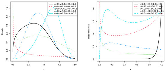
Figure 1. Plots of the pdf and hrf of the EHL-Harris-W distribution.

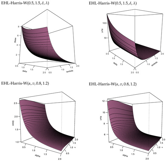
Figure 2. Three Dimensional plots of the skewness and kurtosis of the EHL-Harris-W distribution for some selected parameter values.

It can be observed that,

• When $\alpha$ and v are fixed, the skewness and kurtosis of EHL-Harris-W are both decreasing functions of $\delta$ and $\lambda$.
• When $\delta$ and $\lambda$ are fixed, the skewness and kurtosis of EHL-Harris-W are both decreasing functions of $\alpha$ and v.

5.2. Exponentiated Half Logistic-Harris-Rayleigh (EHL-Harris-R) Distribution

If we consider the Rayleigh distribution with cdf and pdf given by $G(x;\lambda )=1-exp\left(\frac{-x^2}{2{\lambda }^2}\right)$ and $g(x;\lambda )=\frac{x}{{\lambda }^2}exp\left(\frac{-x^2}{2{\lambda }^2}\right)$, respectively, for $\lambda >0$ and $x>0$, then, the EHL-Harris-R distribution has cdf and pdf given by:

$$F(x;\alpha ,v,\delta ,\lambda )={\left[\frac{1-{\left(\frac{\delta exp\left(\frac{-v{x}^2}{2{\lambda }^2}\right)}{1-\overline{\delta }exp\left(\frac{-v{x}^2}{2{\lambda }^2}\right)}\right)}^{\frac{1}{v}}}{1+{\left(\frac{\delta exp\left(\frac{-v{x}^2}{2{\lambda }^2}\right)}{1-\overline{\delta }exp\left(\frac{-v{x}^2}{2{\lambda }^2}\right)}\right)}^{\frac{1}{v}}}\right]}^{\alpha },$$

and

$$\begin{array}{ccc}\hfill f(x;\alpha ,v,\delta ,\lambda )& =& 2\alpha {\delta }^{\frac{1}{v}}\frac{x}{{\lambda }^2}exp\left(\frac{-x^2}{2{\lambda }^2}\right){\left(1-\overline{\delta }exp\left(\frac{-v{x}^2}{2{\lambda }^2}\right)\right)}^{-(\frac{1}{v}+1)}\hfill \\ & \times & {\left[1-{\left(\frac{\delta exp\left(\frac{-v{x}^2}{2{\lambda }^2}\right)}{1-\overline{\delta }exp\left(\frac{-v{x}^2}{2{\lambda }^2}\right)}\right)}^{\frac{1}{v}}\right]}^{\alpha -1}{\left[1+{\left(\frac{\delta exp\left(\frac{-v{x}^2}{2{\lambda }^2}\right)}{1-\overline{\delta }exp\left(\frac{-v{x}^2}{2{\lambda }^2}\right)}\right)}^{\frac{1}{v}}\right]}^{-(\alpha +1)},\hfill \end{array}$$

for $\alpha ,v,\delta ,\lambda >0$ and $\overline{\delta }=1-\delta ,$ $x>0$, respectively The corresponding hrf is given by:

$$\begin{array}{ccc}\hfill h\left(x\right)& =& 2\alpha {\delta }^{\frac{1}{v}}\frac{x}{{\lambda }^2}exp\left(\frac{-x^2}{2{\lambda }^2}\right){\left(1-\overline{\delta }exp\left(\frac{-v{x}^2}{2{\lambda }^2}\right)\right)}^{-(\frac{1}{v}+1)}\hfill \\ & \times & {\left[1-{\left(\frac{\delta exp\left(\frac{-v{x}^2}{2{\lambda }^2}\right)}{1-\overline{\delta }exp\left(\frac{-v{x}^2}{2{\lambda }^2}\right)}\right)}^{\frac{1}{v}}\right]}^{\alpha -1}{\left[1+{\left(\frac{\delta exp\left(\frac{-v{x}^2}{2{\lambda }^2}\right)}{1-\overline{\delta }exp\left(\frac{-v{x}^2}{2{\lambda }^2}\right)}\right)}^{\frac{1}{v}}\right]}^{-(\alpha +1)}\hfill \\ & \times & {\left(1-{\left[\frac{1-{\left(\frac{\delta exp\left(\frac{-v{x}^2}{2{\lambda }^2}\right)}{1-\overline{\delta }exp\left(\frac{-v{x}^2}{2{\lambda }^2}\right)}\right)}^{\frac{1}{v}}}{1+{\left(\frac{\delta exp\left(\frac{-v{x}^2}{2{\lambda }^2}\right)}{1-\overline{\delta }exp\left(\frac{-v{x}^2}{2{\lambda }^2}\right)}\right)}^{\frac{1}{v}}}\right]}^{\alpha }\right)}^{-1},\hfill \end{array}$$

for $\alpha ,v,\delta ,\lambda >0$ and $\overline{\delta }=1-\delta ,$ $x>0.$

Figure 3 shows the plots of the pdf and the hrf of the EHL-Harris-R distribution for different parameter values.The pdf can take various shapes, such as uni-modal and left- or right-skewed. Graphs of the hrf exhibit different shapes, such as increasing, decreasing, bathtub, bathtub followed by upside-down bathtub, and upside-down bathtub followed by bathtub shapes. Figure 4 shows that the EHL-Harris-R distribution can model data sets with different levels of skewness and kurtosis.

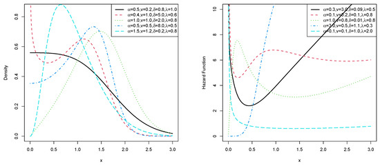
Figure 3. Plots of the pdf and hrf of the EHL-Harris-R distribution.

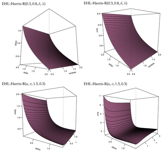
Figure 4. Three Dimensional plots of the skewness and kurtosis of the EHL-Harris-R distribution for some selected parameter values.

It can be observed that.

• When $\alpha$ and v and are fixed, both the skewness and kurtosis of EHL-Harris-R decreases for varying values of $\delta$ and $\lambda$.
• When $\delta$ and $\lambda$ are fixed, both the skewness and kurtosis of EHL-Harris-R decreases for varying values of $\alpha$ and v.

5.3. Exponentiated Half Logistic-Harris-Uniform (EHL-Harris-U) Distribution

If we consider the Uniform distribution with cdf and pdf given by $G(x;\lambda )=\frac{x}{\lambda }$ and $g(x;\lambda )=\frac{1}{\lambda }$, respectively, for $\lambda >0$ and $0<x<\lambda$, then, the EHL-Harris-U distribution has cdf and pdf given by:

$$F(x;\alpha ,v,\delta ,\lambda )={\left[\frac{1-{\left(\frac{\delta {(1-\frac{x}{\lambda })}^v}{1-\overline{\delta }{(1-\frac{x}{\lambda })}^v}\right)}^{\frac{1}{v}}}{1+{\left(\frac{\delta {(1-\frac{x}{\lambda })}^v}{1-\overline{\delta }{(1-\frac{x}{\lambda })}^v}\right)}^{\frac{1}{v}}}\right]}^{\alpha },$$

and

$$\begin{array}{ccc}\hfill f(x;\alpha ,v,\delta ,\lambda )& =& 2\alpha {\delta }^{\frac{1}{v}}\frac{1}{\lambda }{\left(1-\overline{\delta }{\left(1-\frac{x}{\lambda }\right)}^v\right)}^{-(\frac{1}{v}+1)}{\left[1-{\left(\frac{\delta {(1-\frac{x}{\lambda })}^v}{1-\overline{\delta }{(1-\frac{x}{\lambda })}^v}\right)}^{\frac{1}{v}}\right]}^{\alpha -1}\hfill \\ & \times & {\left[1+{\left(\frac{\delta {(1-\frac{x}{\lambda })}^v}{1-\overline{\delta }{(1-\frac{x}{\lambda })}^v}\right)}^{\frac{1}{v}}\right]}^{-(\alpha +1)},\hfill \end{array}$$

for $\alpha ,v,\delta ,\lambda >0$ and $\overline{\delta }=1-\delta ,$ $x>0$, respectively The hrf of the EHL-Harris-U distribution is given by:

$$\begin{array}{ccc}\hfill h\left(x\right)& =& 2\alpha {\delta }^{\frac{1}{v}}\frac{1}{\lambda }{\left(1-\overline{\delta }{\left(1-\frac{x}{\lambda }\right)}^v\right)}^{-(\frac{1}{v}+1)}{\left[1-{\left(\frac{\delta {(1-\frac{x}{\lambda })}^v}{1-\overline{\delta }{(1-\frac{x}{\lambda })}^v}\right)}^{\frac{1}{v}}\right]}^{\alpha -1}\hfill \\ & \times & {\left[1+{\left(\frac{\delta {(1-\frac{x}{\lambda })}^v}{1-\overline{\delta }{(1-\frac{x}{\lambda })}^v}\right)}^{\frac{1}{v}}\right]}^{-(\alpha +1)}{\left(1-{\left[\frac{1-{\left(\frac{\delta {(1-\frac{x}{\lambda })}^v}{1-\overline{\delta }{(1-\frac{x}{\lambda })}^v}\right)}^{\frac{1}{v}}}{1+{\left(\frac{\delta {(1-\frac{x}{\lambda })}^v}{1-\overline{\delta }{(1-\frac{x}{\lambda })}^v}\right)}^{\frac{1}{v}}}\right]}^{\alpha }\right)}^{-1},\hfill \end{array}$$

for $\alpha ,v,\delta ,\lambda >0$ and $\overline{\delta }=1-\delta ,$ $x>0.$

Figure 5 shows the plots of the pdf and the hrf of the EHL-Harris-U distribution for different parameter values. The pdf for the EHL-Harris-U distribution can be J, reverse-J, uni-modal, right-skewed, and  U-shaped. Graphs of the hrf exhibit increasing, decreasing, bathtub, and upside-down bathtub followed by bathtub shapes.

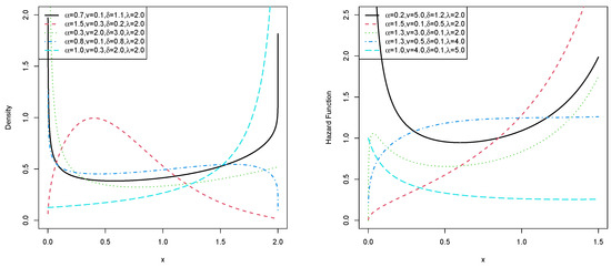
Figure 5. Plots of the pdf and hrf of the EHL-Harris-Uniform distribution.

6. Monte Carlo Simulation Study

With the six estimation methods discussed in Section 4, the performance of the EHL-Harris-W distribution was examined by conducting various simulations for different sizes (n = 25, 50, 100, 200, 400, 800) via the R software. We simulated $N=1000$ samples for the true parameter values of $(\alpha ,v,\delta ,\lambda )$, given in Table 1 and Table 2. The tables list the average bias (ABIAS) and root mean squared errors (RMSEs) for the six estimation methods, withdifferent sample sizes: MLE, LS, WLS, MPS, CVM, and AD. The ABIAS and RMSE for the estimated parameter, say, $\widehat{\theta }$, are, respectively, given by:

$$ABIAS\left(\widehat{\theta }\right)=\frac{{\sum }_{i=1}^N{\widehat{\theta }}_i}{N}-\theta ,\mathrm{and}RMSE\left(\widehat{\theta }\right)=\sqrt{\frac{{\sum }_{i=1}^N{({\widehat{\theta }}_i-\theta )}^2}{N}},$$

Table 1. Simulation Results for Different Estimation Methods for $\alpha =0.5,v=0.8,\delta =0.2,\lambda =1.2$.

		MLE		LS		WLS		MPS		CVM		AD
n	Parameter	ABIAS	RMSE	ABIAS	RMSE	ABIAS	RMSE	ABIAS	RMSE	ABIAS	RMSE	ABIAS	RMSE
25	$\alpha$	$0.{3600}^{\left\{2\right\}}$	$1.{5575}^{\left\{3\right\}}$	$0.{4262}^{\left\{3\right\}}$	$1.{3222}^{\left\{1\right\}}$	$1.{8989}^{\left\{6\right\}}$	$7.{32}^{\left\{6\right\}}$	$0.{3414}^{\left\{1\right\}}$	$1.{9367}^{\left\{4\right\}}$	$0.{4874}^{\left\{4\right\}}$	$1.{4797}^{\left\{2\right\}}$	$1.{0906}^{\left\{5\right\}}$	$5.{5772}^{\left\{5\right\}}$
	v	$0.{8362}^{\left\{3\right\}}$	$1.{6809}^{\left\{2\right\}}$	$0.{7135}^{\left\{2\right\}}$	$2.{7194}^{\left\{4\right\}}$	$0.{2279}^{\left\{1\right\}}$	$1.{2086}^{\left\{1\right\}}$	$1.{1093}^{\left\{6\right\}}$	$2.{5522}^{\left\{3\right\}}$	$1.{0271}^{\left\{5\right\}}$	$3.{3441}^{\left\{5\right\}}$	$0.{9033}^{\left\{4\right\}}$	$3.{6736}^{\left\{6\right\}}$
	$\delta$	$-0.{0468}^{\left\{3\right\}}$	$0.{1560}^{\left\{1\right\}}$	$0.{0440}^{\left\{2\right\}}$	$0.{4773}^{\left\{4\right\}}$	$0.{0295}^{\left\{1\right\}}$	$0.{2730}^{\left\{3\right\}}$	$-0.{0793}^{\left\{4\right\}}$	$0.{1807}^{\left\{2\right\}}$	$0.{5815}^{\left\{6\right\}}$	$13.{1361}^{\left\{6\right\}}$	$0.{3000}^{\left\{5\right\}}$	$6.{0538}^{\left\{5\right\}}$
	$\lambda$	$0.{2422}^{\left\{5\right\}}$	$0.{6298}^{\left\{2\right\}}$	$0.{0350}^{\left\{1\right\}}$	$0.{6690}^{\left\{3\right\}}$	$0.{0816}^{\left\{2\right\}}$	$0.{3520}^{\left\{1\right\}}$	$0.{5238}^{\left\{6\right\}}$	$0.{8578}^{\left\{6\right\}}$	$0.{2066}^{\left\{4\right\}}$	$0.{7601}^{\left\{5\right\}}$	$0.{1032}^{\left\{3\right\}}$	$0.{7464}^{\left\{4\right\}}$
∑ ranks		21		20		21		32		37		37
50	$\alpha$	$0.{0919}^{\left\{2\right\}}$	$0.{4452}^{\left\{2\right\}}$	$0.{1614}^{\left\{3\right\}}$	$0.{4813}^{\left\{3\right\}}$	$0.{7798}^{\left\{6\right\}}$	$4.{2968}^{\left\{6\right\}}$	$0.{0330}^{\left\{1\right\}}$	$0.{3327}^{\left\{1\right\}}$	$0.{4210}^{\left\{4\right\}}$	$1.{3092}^{\left\{4\right\}}$	$0.{4718}^{\left\{5\right\}}$	$2.{2390}^{\left\{5\right\}}$
	v	$0.{5754}^{\left\{4\right\}}$	$1.{2534}^{\left\{2\right\}}$	$0.{3888}^{\left\{2\right\}}$	$2.{0828}^{\left\{6\right\}}$	$0.{1732}^{\left\{1\right\}}$	$0.{8370}^{\left\{1\right\}}$	$1.{0991}^{\left\{6\right\}}$	$1.{8791}^{\left\{3\right\}}$	$0.{7734}^{\left\{5\right\}}$	$2.{0702}^{\left\{5\right\}}$	$0.{5615}^{\left\{3\right\}}$	$2.{0279}^{\left\{4\right\}}$
	$\delta$	$-0.{0350}^{\left\{5\right\}}$	$0.{1256}^{\left\{2\right\}}$	$0.{0202}^{\left\{2\right\}}$	$0.{1253}^{\left\{1\right\}}$	$0.{0085}^{\left\{1\right\}}$	$0.{1369}^{\left\{4\right\}}$	$-0.{0735}^{\left\{6\right\}}$	$0.{1274}^{\left\{3\right\}}$	$0.{0341}^{\left\{4\right\}}$	$1.{6383}^{\left\{6\right\}}$	$0.{0309}^{\left\{3\right\}}$	$1.{1273}^{\left\{5\right\}}$
	$\lambda$	$0.{1983}^{\left\{4\right\}}$	$0.{5088}^{\left\{2\right\}}$	$0.{0280}^{\left\{1\right\}}$	$0.{5230}^{\left\{3\right\}}$	$0.{0560}^{\left\{2\right\}}$	$0.{2592}^{\left\{1\right\}}$	$0.{4922}^{\left\{6\right\}}$	$0.{7338}^{\left\{6\right\}}$	$0.{2081}^{\left\{5\right\}}$	$0.{7081}^{\left\{5\right\}}$	$0.{0599}^{\left\{3\right\}}$	$0.{6020}^{\left\{4\right\}}$
∑ ranks		23		21		22		32		38		32
100	$\alpha$	$0.{0357}^{\left\{2\right\}}$	$0.{1886}^{\left\{2\right\}}$	$0.{0962}^{\left\{3\right\}}$	$0.{3638}^{\left\{4\right\}}$	$0.{3597}^{\left\{5\right\}}$	$1.{2375}^{\left\{6\right\}}$	$-0.{0316}^{\left\{1\right\}}$	$0.{1725}^{\left\{1\right\}}$	$0.{3675}^{\left\{6\right\}}$	$1.{0812}^{\left\{5\right\}}$	$0.{1089}^{\left\{4\right\}}$	$0.{2695}^{\left\{3\right\}}$
	v	$0.{3262}^{\left\{4\right\}}$	$0.{8084}^{\left\{2\right\}}$	$0.{1545}^{\left\{3\right\}}$	$1.{0094}^{\left\{4\right\}}$	$0.{0877}^{\left\{2\right\}}$	$0.{6300}^{\left\{1\right\}}$	$0.{6849}^{\left\{6\right\}}$	$1.{1170}^{\left\{5\right\}}$	$0.{6116}^{\left\{5\right\}}$	$1.{9749}^{\left\{6\right\}}$	$0.{0368}^{\left\{1\right\}}$	$0.{8146}^{\left\{3\right\}}$
	$\delta$	$-0.{0206}^{\left\{5\right\}}$	$0.{0877}^{\left\{1\right\}}$	$0.{0157}^{\left\{3\right\}}$	$0.{1037}^{\left\{5\right\}}$	$0.{0028}^{\left\{1\right\}}$	$0.{0970}^{\left\{2\right\}}$	$-0.{0562}^{\left\{6\right\}}$	$0.{0995}^{\left\{3\right\}}$	$0.{0146}^{\left\{2\right\}}$	$0.{5774}^{\left\{6\right\}}$	$0.{0188}^{\left\{4\right\}}$	$0.{0996}^{\left\{4\right\}}$
	$\lambda$	$0.{0923}^{\left\{4\right\}}$	$0.{3401}^{\left\{2\right\}}$	$0.{0236}^{\left\{2\right\}}$	$0.{4358}^{\left\{4\right\}}$	$0.{0151}^{\left\{1\right\}}$	$0.{1885}^{\left\{1\right\}}$	$0.{3652}^{\left\{6\right\}}$	$0.{5342}^{\left\{5\right\}}$	$0.{1487}^{\left\{5\right\}}$	$0.{6439}^{\left\{6\right\}}$	$-0.{0472}^{\left\{3\right\}}$	$0.{3790}^{\left\{3\right\}}$
∑ ranks		22		28		19		33		41		25
200	$\alpha$	$0.{0287}^{\left\{1\right\}}$	$0.{1589}^{\left\{2\right\}}$	$0.{0571}^{\left\{4\right\}}$	$0.{2059}^{\left\{4\right\}}$	$0.{1461}^{\left\{6\right\}}$	$0.{5516}^{\left\{6\right\}}$	$-0.{0447}^{\left\{2\right\}}$	$0.{1171}^{\left\{1\right\}}$	$0.{0514}^{\left\{3\right\}}$	$0.{2139}^{\left\{5\right\}}$	$0.{0709}^{\left\{5\right\}}$	$0.{1808}^{\left\{3\right\}}$
	v	$0.{1670}^{\left\{5\right\}}$	$0.{5780}^{\left\{2\right\}}$	$0.{1043}^{\left\{3\right\}}$	$0.{8099}^{\left\{5\right\}}$	$0.{0966}^{\left\{2\right\}}$	$0.{5064}^{\left\{1\right\}}$	$0.{4459}^{\left\{6\right\}}$	$0.{7267}^{\left\{4\right\}}$	$0.{1344}^{\left\{4\right\}}$	$0.{8458}^{\left\{6\right\}}$	$-0.{0310}^{\left\{1\right\}}$	$0.{6005}^{\left\{3\right\}}$
	$\delta$	$-0.{0112}^{\left\{3\right\}}$	$0.{0686}^{\left\{1\right\}}$	$0.{0154}^{\left\{4\right\}}$	$0.{0855}^{\left\{6\right\}}$	$-0.{0038}^{\left\{1\right\}}$	$0.{0771}^{\left\{4\right\}}$	$-0.{0380}^{\left\{6\right\}}$	$0.{0747}^{\left\{2\right\}}$	$0.{0096}^{\left\{2\right\}}$	$0.{0850}^{\left\{5\right\}}$	$0.{0169}^{\left\{5\right\}}$	$0.{0768}^{\left\{3\right\}}$
	$\lambda$	$0.{0506}^{\left\{4\right\}}$	$0.{2893}^{\left\{2\right\}}$	$0.{0140}^{\left\{1\right\}}$	$0.{3885}^{\left\{5\right\}}$	$0.{0222}^{\left\{2\right\}}$	$0.{1596}^{\left\{1\right\}}$	$0.{2501}^{\left\{6\right\}}$	$0.{3838}^{\left\{4\right\}}$	$0.{0448}^{\left\{3\right\}}$	$0.{4060}^{\left\{6\right\}}$	$-0.{0529}^{\left\{5\right\}}$	$0.{3064}^{\left\{3\right\}}$
∑ ranks		20		32		23		31		34		28
400	$\alpha$	$0.{0270}^{\left\{1\right\}}$	$0.{1231}^{\left\{2\right\}}$	$0.{0519}^{\left\{4\right\}}$	$0.{1776}^{\left\{5\right\}}$	$0.{0809}^{\left\{6\right\}}$	$0.{3784}^{\left\{6\right\}}$	$-0.{0314}^{\left\{2\right\}}$	$0.{1013}^{\left\{1\right\}}$	$0.{0354}^{\left\{3\right\}}$	$0.{1719}^{\left\{4\right\}}$	$0.{0580}^{\left\{5\right\}}$	$0.{1520}^{\left\{3\right\}}$
	v	$0.{0739}^{\left\{3\right\}}$	$0.{4242}^{\left\{2\right\}}$	$0.{0284}^{\left\{1\right\}}$	$0.{6396}^{\left\{5\right\}}$	$0.{0768}^{\left\{4\right\}}$	$0.{4087}^{\left\{1\right\}}$	$0.{2737}^{\left\{6\right\}}$	$0.{5002}^{\left\{3\right\}}$	$0.{1072}^{\left\{5\right\}}$	$0.{6804}^{\left\{6\right\}}$	$-0.{0286}^{\left\{2\right\}}$	$0.{5800}^{\left\{4\right\}}$
	$\delta$	$-0.{0039}^{\left\{2\right\}}$	$0.{0550}^{\left\{1\right\}}$	$0.{0143}^{\left\{5\right\}}$	$0.{0669}^{\left\{4\right\}}$	$-0.{0033}^{\left\{1\right\}}$	$0.{0635}^{\left\{3\right\}}$	$-0.{0230}^{\left\{6\right\}}$	$0.{0553}^{\left\{2\right\}}$	$0.{0063}^{\left\{3\right\}}$	$0.{0700}^{\left\{5\right\}}$	$0.{0117}^{\left\{4\right\}}$	$0.{0745}^{\left\{6\right\}}$
	$\lambda$	$0.{0092}^{\left\{1\right\}}$	$0.{2249}^{\left\{2\right\}}$	$-0.{0162}^{\left\{2\right\}}$	$0.{3419}^{\left\{5\right\}}$	$0.{0166}^{\left\{3\right\}}$	$0.{1300}^{\left\{1\right\}}$	$0.{1602}^{\left\{6\right\}}$	$0.{2772}^{\left\{3\right\}}$	$0.{0395}^{\left\{4\right\}}$	$0.{3694}^{\left\{6\right\}}$	$-0.{0521}^{\left\{5\right\}}$	$0.{3060}^{\left\{4\right\}}$
∑ ranks		14		31		25		29		36		33
800	$\alpha$	$0.{0230}^{\left\{2\right\}}$	$0.{0993}^{\left\{2\right\}}$	$0.{0395}^{\left\{5\right\}}$	$0.{1445}^{\left\{4\right\}}$	$0.{0698}^{\left\{6\right\}}$	$0.{3061}^{\left\{6\right\}}$	$-0.{0212}^{\left\{1\right\}}$	$0.{0712}^{\left\{1\right\}}$	$0.{0327}^{\left\{4\right\}}$	$0.{1429}^{\left\{3\right\}}$	$0.{0301}^{\left\{3\right\}}$	$0.{1509}^{\left\{5\right\}}$
	v	$0.{0372}^{\left\{3\right\}}$	$0.{3227}^{\left\{2\right\}}$	$0.{0047}^{\left\{1\right\}}$	$0.{5271}^{\left\{6\right\}}$	$0.{0373}^{\left\{4\right\}}$	$0.{2998}^{\left\{1\right\}}$	$0.{1667}^{\left\{6\right\}}$	$0.{3355}^{\left\{3\right\}}$	$0.{0424}^{\left\{5\right\}}$	$0.{5260}^{\left\{5\right\}}$	$-0.{0074}^{\left\{2\right\}}$	$0.{4708}^{\left\{4\right\}}$
	$\delta$	$0.{0003}^{\left\{1\right\}}$	$0.{0416}^{\left\{2\right\}}$	$0.{0124}^{\left\{4.5\right\}}$	$0.{0577}^{\left\{5\right\}}$	$-0.{0023}^{\left\{2\right\}}$	$0.{0480}^{\left\{3\right\}}$	$-0.{0160}^{\left\{6\right\}}$	$0.{0411}^{\left\{1\right\}}$	$0.{0062}^{\left\{3\right\}}$	$0.{0564}^{\left\{4\right\}}$	$0.{0124}^{\left\{4.5\right\}}$	$0.{0612}^{\left\{6\right\}}$
	$\lambda$	$-0.{0075}^{\left\{3\right\}}$	$0.{1791}^{\left\{2\right\}}$	$-0.{0149}^{\left\{4\right\}}$	$0.{3088}^{\left\{6\right\}}$	$0.{005}^{\left\{1\right\}}$	$0.{1026}^{\left\{1\right\}}$	$0.{0946}^{\left\{6\right\}}$	$0.{1876}^{\left\{3\right\}}$	$0.{0057}^{\left\{2\right\}}$	$0.{3064}^{\left\{5\right\}}$	$-0.{0506}^{\left\{5\right\}}$	$0.{2631}^{\left\{4\right\}}$
∑ ranks		17		35.5		24		27		31		33.5

Table 2. Simulation Results for Different Estimation Methods for $\alpha =1.3,v=0.5,\delta =0.2,\lambda =0.5.$.

		MLE		LS		WLS		MPS		CVM		AD
n	Parameter	ABIAS	RMSE	ABIAS	RMSE	ABIAS	RMSE	ABIAS	RMSE	ABIAS	RMSE	ABIAS	RMSE
25	$\alpha$	$3.{2027}^{\left\{6\right\}}$	$24.{7796}^{\left\{6\right\}}$	$0.{8518}^{\left\{1\right\}}$	$2.{9938}^{\left\{1\right\}}$	$1.{8989}^{\left\{4\right\}}$	$7.{3200}^{\left\{3\right\}}$	$2.{2549}^{\left\{5\right\}}$	$18.{6595}^{\left\{5\right\}}$	$1.{0141}^{\left\{2\right\}}$	$4.{2837}^{\left\{2\right\}}$	$1.{6051}^{\left\{3\right\}}$	$8.{2479}^{\left\{4\right\}}$
	v	$0.{6803}^{\left\{4\right\}}$	$1.{2559}^{\left\{3\right\}}$	$0.{4755}^{\left\{3\right\}}$	$1.{8412}^{\left\{5\right\}}$	$0.{2279}^{\left\{1\right\}}$	$1.{2086}^{\left\{1\right\}}$	$1.{0499}^{\left\{6\right\}}$	$1.{8359}^{\left\{4\right\}}$	$0.{9181}^{\left\{5\right\}}$	$3.{3558}^{\left\{6\right\}}$	$0.{3512}^{\left\{2\right\}}$	$1.{2549}^{\left\{2\right\}}$
	$\delta$	$-0.{0520}^{\left\{3\right\}}$	$0.{1906}^{\left\{2\right\}}$	$0.{1021}^{\left\{6\right\}}$	$1.{2825}^{\left\{5\right\}}$	$0.{0295}^{\left\{2\right\}}$	$0.{2730}^{\left\{3\right\}}$	$-0.{0873}^{\left\{5\right\}}$	$0.{1812}^{\left\{1\right\}}$	$0.{0846}^{\left\{4\right\}}$	$1.{2952}^{\left\{6\right\}}$	$0.{0288}^{\left\{1\right\}}$	$0.{9057}^{\left\{4\right\}}$
	$\lambda$	$0.{2400}^{\left\{4\right\}}$	$0.{4189}^{\left\{3\right\}}$	$0.{1539}^{\left\{3\right\}}$	$0.{4452}^{\left\{4\right\}}$	$0.{0816}^{\left\{1\right\}}$	$0.{3520}^{\left\{1\right\}}$	$0.{4472}^{\left\{6\right\}}$	$0.{6379}^{\left\{5\right\}}$	$0.{3394}^{\left\{5\right\}}$	$0.{6529}^{\left\{6\right\}}$	$0.{1245}^{\left\{2\right\}}$	$0.{3685}^{\left\{2\right\}}$
∑ ranks		31		28		16		37		36		20
50	$\alpha$	$0.{5060}^{\left\{2\right\}}$	$2.{8053}^{\left\{2\right\}}$	$0.{7239}^{\left\{3\right\}}$	$2.{821}^{\left\{3\right\}}$	$0.{7798}^{\left\{4\right\}}$	$4.{2968}^{\left\{5\right\}}$	$0.{3971}^{\left\{1\right\}}$	$2.{1083}^{\left\{1\right\}}$	$0.{8636}^{\left\{5\right\}}$	$3.{1983}^{\left\{4\right\}}$	$0.{9481}^{\left\{6\right\}}$	$5.{8778}^{\left\{6\right\}}$
	v	$0.{4682}^{\left\{5\right\}}$	$0.{9117}^{\left\{3\right\}}$	$0.{2923}^{\left\{3\right\}}$	$1.{2776}^{\left\{6\right\}}$	$0.{1732}^{\left\{1\right\}}$	$0.{837}^{\left\{2\right\}}$	$0.{7795}^{\left\{6\right\}}$	$1.{2334}^{\left\{4\right\}}$	$0.{4361}^{\left\{4\right\}}$	$1.{2602}^{\left\{5\right\}}$	$0.{1734}^{\left\{2\right\}}$	$0.{7184}^{\left\{1\right\}}$
	$\delta$	$-0.{0411}^{\left\{5\right\}}$	$0.{1295}^{\left\{2\right\}}$	$0.{0138}^{\left\{3\right\}}$	$0.{1545}^{\left\{6\right\}}$	$0.{0085}^{\left\{2\right\}}$	$0.{1369}^{\left\{4\right\}}$	$-0.{0817}^{\left\{6\right\}}$	$0.{1423}^{\left\{5\right\}}$	$-0.{0218}^{\left\{4\right\}}$	$0.{1368}^{\left\{3\right\}}$	$-0.{0057}^{\left\{1\right\}}$	$0.{1251}^{\left\{1\right\}}$
	$\lambda$	$0.{1544}^{\left\{4\right\}}$	$0.{2926}^{\left\{3\right\}}$	$0.{1002}^{\left\{3\right\}}$	$0.{3362}^{\left\{4\right\}}$	$0.{056}^{\left\{1\right\}}$	$0.{2592}^{\left\{2\right\}}$	$0.{2856}^{\left\{6\right\}}$	$0.{4199}^{\left\{6\right\}}$	$0.{1706}^{\left\{5\right\}}$	$0.{4066}^{\left\{5\right\}}$	$0.{0629}^{\left\{2\right\}}$	$0.{2459}^{\left\{1\right\}}$
∑ ranks		26		31		21		35		35		20
100	$\alpha$	$0.{1576}^{\left\{3\right\}}$	$0.{8685}^{\left\{2\right\}}$	$0.{128}^{\left\{1\right\}}$	$0.{6969}^{\left\{1\right\}}$	$0.{3597}^{\left\{6\right\}}$	$1.{2375}^{\left\{5\right\}}$	$0.{1297}^{\left\{2\right\}}$	$0.{995}^{\left\{4\right\}}$	$0.{2925}^{\left\{5\right\}}$	$1.{3661}^{\left\{6\right\}}$	$0.{2657}^{\left\{4\right\}}$	$0.{9102}^{\left\{3\right\}}$
	v	$0.{3051}^{\left\{5\right\}}$	$0.{6629}^{\left\{3\right\}}$	$0.{2182}^{\left\{3\right\}}$	$0.{6918}^{\left\{4\right\}}$	$0.{0877}^{\left\{1\right\}}$	$0.{63}^{\left\{2\right\}}$	$0.{5589}^{\left\{6\right\}}$	$0.{8568}^{\left\{5\right\}}$	$0.{3045}^{\left\{4\right\}}$	$1.{065}^{\left\{6\right\}}$	$0.{1077}^{\left\{2\right\}}$	$0.{5677}^{\left\{1\right\}}$
	$\delta$	$-0.{0325}^{\left\{5\right\}}$	$0.{0966}^{\left\{3\right\}}$	$-0.{0132}^{\left\{3\right\}}$	$0.{0896}^{\left\{1\right\}}$	$0.{0028}^{\left\{1\right\}}$	$0.{097}^{\left\{4\right\}}$	$-0.{0674}^{\left\{6\right\}}$	$0.{1156}^{\left\{6\right\}}$	$-0.{0162}^{\left\{4\right\}}$	$0.{1102}^{\left\{5\right\}}$	$-0.{0043}^{\left\{2\right\}}$	$0.{0943}^{\left\{2\right\}}$
	$\lambda$	$0.{0903}^{\left\{4\right\}}$	$0.{2007}^{\left\{3\right\}}$	$0.{0646}^{\left\{3\right\}}$	$0.{2219}^{\left\{4\right\}}$	$0.{0151}^{\left\{1\right\}}$	$0.{1885}^{\left\{2\right\}}$	$0.{1868}^{\left\{6\right\}}$	$0.{2725}^{\left\{5\right\}}$	$0.{1138}^{\left\{5\right\}}$	$0.{3007}^{\left\{6\right\}}$	$0.{0293}^{\left\{2\right\}}$	$0.{1779}^{\left\{1\right\}}$
∑ ranks		28		20		22		40		41		17
200	$\alpha$	$0.{0582}^{\left\{2\right\}}$	$0.{5537}^{\left\{5\right\}}$	$0.{0856}^{\left\{3\right\}}$	$0.{5115}^{\left\{2\right\}}$	$0.{1461}^{\left\{6\right\}}$	$0.{5516}^{\left\{4\right\}}$	$-0.{0334}^{\left\{1\right\}}$	$0.{4822}^{\left\{1\right\}}$	$0.{1284}^{\left\{4\right\}}$	$0.{6956}^{\left\{6\right\}}$	$0.{1442}^{\left\{5\right\}}$	$0.{5209}^{\left\{3\right\}}$
	v	$0.{1986}^{\left\{4\right\}}$	$0.{4754}^{\left\{2\right\}}$	$0.{1653}^{\left\{3\right\}}$	$0.{5687}^{\left\{4\right\}}$	$0.{0966}^{\left\{2\right\}}$	$0.{5064}^{\left\{3\right\}}$	$0.{3957}^{\left\{6\right\}}$	$0.{6052}^{\left\{5\right\}}$	$0.{2022}^{\left\{5\right\}}$	$0.{7013}^{\left\{6\right\}}$	$0.{0706}^{\left\{1\right\}}$	$0.{4597}^{\left\{1\right\}}$
	$\delta$	$-0.{0212}^{\left\{5\right\}}$	$0.{0716}^{\left\{1\right\}}$	$-0.{0110}^{\left\{3\right\}}$	$0.{079}^{\left\{4\right\}}$	$-0.{0038}^{\left\{2\right\}}$	$0.{0771}^{\left\{3\right\}}$	$-0.{0509}^{\left\{6\right\}}$	$0.{0842}^{\left\{5\right\}}$	$-0.{0123}^{\left\{4\right\}}$	$0.{0931}^{\left\{6\right\}}$	$-0.{0025}^{\left\{1\right\}}$	$0.{0756}^{\left\{2\right\}}$
	$\lambda$	$0.{0572}^{\left\{4\right\}}$	$0.{1512}^{\left\{2\right\}}$	$0.{0485}^{\left\{3\right\}}$	$0.{1841}^{\left\{4\right\}}$	$0.{0222}^{\left\{2\right\}}$	$0.{1596}^{\left\{3\right\}}$	$0.{1267}^{\left\{6\right\}}$	$0.{1939}^{\left\{5\right\}}$	$0.{0709}^{\left\{5\right\}}$	$0.{2285}^{\left\{6\right\}}$	$0.{0147}^{\left\{1\right\}}$	$0.{1437}^{\left\{1\right\}}$
∑ ranks		25		26		25		35		42		15
400	$\alpha$	$0.{0426}^{\left\{1\right\}}$	$0.{3817}^{\left\{3\right\}}$	$0.{0523}^{\left\{4\right\}}$	$0.{4195}^{\left\{4.5\right\}}$	$0.{0809}^{\left\{5\right\}}$	$0.{3784}^{\left\{2\right\}}$	$-0.{0493}^{\left\{3\right\}}$	$0.{3049}^{\left\{1\right\}}$	$0.{0427}^{\left\{2\right\}}$	$0.{4305}^{\left\{6\right\}}$	$0.{1101}^{\left\{6\right\}}$	$0.{4195}^{\left\{4.5\right\}}$
	v	$0.{1245}^{\left\{3\right\}}$	$0.{3493}^{\left\{1\right\}}$	$0.{1437}^{\left\{4\right\}}$	$0.{5051}^{\left\{5\right\}}$	$0.{0768}^{\left\{2\right\}}$	$0.{4087}^{\left\{4\right\}}$	$0.{2317}^{\left\{6\right\}}$	$0.{3848}^{\left\{3\right\}}$	$0.{1554}^{\left\{5\right\}}$	$0.{5236}^{\left\{6\right\}}$	$0.{0588}^{\left\{1\right\}}$	$0.{3730}^{\left\{2\right\}}$
	$\delta$	$-0.{0154}^{\left\{5\right\}}$	$0.{0559}^{\left\{1\right\}}$	$-0.{0107}^{\left\{3\right\}}$	$0.{0712}^{\left\{5\right\}}$	$-0.{0033}^{\left\{1\right\}}$	$0.{0635}^{\left\{4\right\}}$	$-0.{0333}^{\left\{6\right\}}$	$0.{0600}^{\left\{2\right\}}$	$-0.{0124}^{\left\{4\right\}}$	$0.{075}^{\left\{6\right\}}$	$-0.{0042}^{\left\{2\right\}}$	$0.{0608}^{\left\{3\right\}}$
	$\lambda$	$0.{0332}^{\left\{3\right\}}$	$0.{1173}^{\left\{1\right\}}$	$0.{0442}^{\left\{4\right\}}$	$0.{1622}^{\left\{5\right\}}$	$0.{0166}^{\left\{2\right\}}$	$0.{1300}^{\left\{4\right\}}$	$0.{0744}^{\left\{6\right\}}$	$0.{1274}^{\left\{3\right\}}$	$0.{0533}^{\left\{5\right\}}$	$0.{1738}^{\left\{6\right\}}$	$0.{0100}^{\left\{1\right\}}$	$0.{1231}^{\left\{2\right\}}$
∑ ranks		18		34.5		24		30		40		21.5
800	$\alpha$	$0.{0556}^{\left\{4\right\}}$	$0.{3285}^{\left\{4\right\}}$	$0.{0310}^{\left\{2\right\}}$	$0.{3396}^{\left\{5\right\}}$	$0.{0698}^{\left\{5\right\}}$	$0.{3061}^{\left\{2\right\}}$	$-0.{0394}^{\left\{3\right\}}$	$0.{254}^{\left\{1\right\}}$	$0.{0266}^{\left\{1\right\}}$	$0.{3450}^{\left\{6\right\}}$	$0.{0892}^{\left\{6\right\}}$	$0.{3229}^{\left\{3\right\}}$
	v	$0.{0487}^{\left\{3\right\}}$	$0.{2658}^{\left\{1\right\}}$	$0.{1029}^{\left\{4\right\}}$	$0.{3997}^{\left\{5\right\}}$	$0.{0373}^{\left\{2\right\}}$	$0.{2998}^{\left\{4\right\}}$	$0.{1597}^{\left\{6\right\}}$	$0.{2938}^{\left\{3\right\}}$	$0.{1095}^{\left\{5\right\}}$	$0.{4188}^{\left\{6\right\}}$	$0.{0192}^{\left\{1\right\}}$	$0.{2881}^{\left\{2\right\}}$
	$\delta$	$-0.{0047}^{\left\{3\right\}}$	$0.{0448}^{\left\{1\right\}}$	$-0.{0084}^{\left\{4.5\right\}}$	$0.{0595}^{\left\{5\right\}}$	$-0.{0023}^{\left\{2\right\}}$	$0.{048}^{\left\{3\right\}}$	$-0.{0232}^{\left\{6\right\}}$	$0.{0473}^{\left\{2\right\}}$	$-0.{0084}^{\left\{4.5\right\}}$	$0.{0622}^{\left\{6\right\}}$	$0.{0005}^{\left\{1\right\}}$	$0.{0494}^{\left\{4\right\}}$
	$\lambda$	$0.{0105}^{\left\{3\right\}}$	$0.{0951}^{\left\{1\right\}}$	$0.{0318}^{\left\{4\right\}}$	$0.{1372}^{\left\{5\right\}}$	$0.{0050}^{\left\{2\right\}}$	$0.{1026}^{\left\{4\right\}}$	$0.{0510}^{\left\{6\right\}}$	$0.{0993}^{\left\{3\right\}}$	$0.{0352}^{\left\{5\right\}}$	$0.{1417}^{\left\{6\right\}}$	$-0.{0024}^{\left\{1\right\}}$	$0.{0977}^{\left\{2\right\}}$
∑ ranks		20		34.5		24		30		39.5		20

In Table 1 and Table 2, the row indicating ∑ Ranks corresponds to the partial sum of the ranks. Among all the estimators for a given metric, the superscript indicates the rank. Table 1 presents, for example, the ABIAS of $\widehat{\alpha }$, obtained via the MLE method, as $0.{3600}^{\left\{2\right\}}$ for $n=25$. This indicates that the ABIAS of $\widehat{\alpha }$ obtained using the MLE method ranks second among all other estimators. So, when $n=25$, in comparison with all other estimators, MLE provided the second best ABIAS of $\widehat{\alpha }$.

Table 3 shows the partial and overall ranks of all the estimation methods of the EHL-Harris-W distribution by means of various model parameter values. Based on the results in Table 1 and Table 2, the EHL-Harris-W distribution was stable, as the ABIAS and RMSE values for its four parameters were modest. It can be observed that the bias occasionally decreased with increasing sample size, while RMSE decreased as sample size increased for all estimations. Figure 6 and Figure 7 demonstrate how the RMSEs of the parameters decreased with increasing sample size for each estimation method. It appears that, for large sample sizes, all estimation methods provided accurate bias and mean squared error estimates. Table 3 shows that the MLE and WLS methods almost equally allowed us to obtain better estimates of EHL-Harris-W parameters, with MLE ranked first, followed by WLS and, then, by AD. According to the rankings, the CVM method performed the least well.

Table 3. Partial and Overall Ranks of all Estimation Methods of EHL-Harris-W Distribution by Various Model Parameter Values.

Parameters	n	MLE	LS	WLS	MPS	CVM	AD
$\alpha =0.5,v=0.8,\delta =0.2,\lambda =1.2$	25	2.5	1.0	2.5	4.0	5.5	5.5
	50	3.0	1.0	2.0	4.5	6.0	4.5
	100	2.0	4.0	1.0	5.0	6.0	3.0
	200	1.0	5.0	2.0	4.0	6.0	3.0
	400	1.0	5.0	3.0	4.0	6.0	2.0
	800	1.0	5.0	2.0	4.0	6.0	3.0
$\alpha =1.3,v=0.5,\delta =0.2,\lambda =0.5$	25	4.0	3.0	1.0	6.0	5.0	2.0
	50	3.0	4.0	2.0	5.5	5.5	1.0
	100	4.0	2.0	3.0	5.0	6.0	1.0
	200	2.5	4.0	2.5	5.0	6.0	1.0
	400	1.0	5.0	3.0	4.0	6.0	2.0
	800	1.5	5.0	3.0	4.0	6.0	1.5
∑ ranks		26.5	44.0	27.0	55.0	70.0	29.5
Overall rank		1	4	2	5	6	3

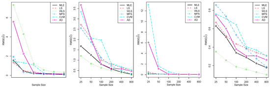
Figure 6. Plots of RMSEs of parameters in Table 1.

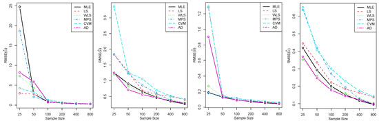
Figure 7. Plots of RMSEs of parameters in Table 2.

7. Actuarial Measures

In this section, we present some risk measures, which are frequently used by financial and actuarial practitioners, to evaluate the exposure to market risk in a portfolio of instruments, and, specifically, the following: value at risk (VaR), tail value at risk (TVaR), tail variance (TV) and tail variance premium (TVP).

7.1. Value at Risk (VaR)

VaR is a widely used actuarial measure, which measures financial market risk. It is also known as the quantile risk measure, or the quantile premium principle, and it is always given with a specified confidence level, for example ($90\%$, $95\%$ or $99\%)$. The VaR for the EHL-Harris-G family of distributions is given by:

$$\begin{array}{ccc}\hfill X_q& =& G^{-1}\left[1-{\left({\left[\frac{1-q^{\frac{1}{\alpha }}}{1+q^{\frac{1}{\alpha }}}\right]}^{-v}\delta +\overline{\delta }\right)}^{-\frac{1}{v}}\right],\hfill \end{array}$$

(24)

where $q\in (0,1)$ is a specified level of significance.

7.2. Tail Value at Risk (TVaR)

The TVaR is also an important and widely used actuarial measure to quantify the expected value of loss were an event outside the specified probability level to occur. It is also known as the conditional tail expectation (CTE), or tail conditional expectation (TCE). For the EHL-Harris-G family of distributions, the TVaR is given by:

$$\begin{array}{ccc}\hfill TVa{R}_q& =& E(X\mid X>x_q)=\frac{1}{1-q}{\int }_{Va{R}_q}^{\infty }xf\left(x\right)dx\hfill \\ & =& \frac{1}{1-q}\sum _{p=0}^{\infty }{\int }_{Va{R}_q}^{\infty }x{\phi }_{p+1}{g}_{p+1}(x;\zeta )dx,\hfill \end{array}$$

(25)

${\phi }_{p+1}$ is given by Equation (11).

7.3. Tail Variance (TV)

The tail variance is one of the most important actuarial measures which looks at the variance beyond the VaR. The TV of the EHL-Harris-G family of distributions can be defined as:

$$\begin{array}{ccc}\hfill T{V}_q& =& E(X^2\mid X>x_q)-{\left(TVa{R}_q\right)}^2\hfill \\ & =& \frac{1}{1-q}{\int }_{Va{R}_q}^{\infty }{x}^{2}f\left(x\right)dx-{\left(TVa{R}_q\right)}^2\hfill \\ & =& \frac{1}{1-q}\sum _{p=0}^{\infty }{\phi }_{p+1}{\int }_{Va{R}_q}^{\infty }{x}^2{g}_{p+1}(x;\zeta )dx-{\left(TVa{R}_q\right)}^2,\hfill \end{array}$$

(26)

where $g_{p+1}(x;\zeta )=(p+1){\left[G(x;\zeta )\right]}^{p}g(x;\zeta )$ is the Exp-G pdf with the power parameter $(p+1)$ and parameter vector $\zeta ,$ and ${\phi }_{p+1}$ is given by Equation (11). Thus, the TV of the EHL-Harris-G family of distributions can be obtained from those of the Exp-G distribution.

7.4. Tail Variance Premium (TVP)

The TVP is an important acturial measure that plays an essential role in insurance sciences. The TVP of the EHL-Harris-G family of distributions takes the form:

$$TV{P}_q=TVa{R}_q+\delta \left(T{V}_q\right),$$

(27)

where $0<\delta <1$. The  TVP of the EHL-Harris-G family of distributions can be obtained by substituting the Equations (25) and (26) into Equation (27).

7.5. Numerical Study for the Risk Measures

The numerical simulations for VaR, TVaR, TV and TVP are presented in this sub-section. The  VaR, TVaR, TV and TVP of the Exponentiated Half Logistic-Harris-W (EHL-Harris-W) distribution were compared with those of its sub-models, namely, HL-Harris-W, EHL-MO-W, HL-W and EHL-W, to assess the roles of additional parameters in modulating the weight of the tails of the newly proposed distribution and the non-nested models, alpha power Topp-Leone Weibull (APTLW) distribution, by [27], and alpha power log-logistic distribution (APExLLD), by [28].

The simulation results were obtained as follows:

1. Random samples of size $n=100$ were generated from each one of the used distributions and parameters estimated via the maximum likelihood method.

2. One thousand repetitions were made to calculate the VaR, TVaR, TV and TVP for these distributions.

Table 4 and Table 5 show the numerical findings of VaR, TVaR, TV and TVP for the five compared distributions. A model with higher values of VaR, TVaR, TV and TVP is said to have a heavier tail. The results given in Table 4 and Table 5 show that the EHL-Harris-W distribution had heavier tails than those of the HL-Harris-W, EHL-MO-W, HL-W, EHL-W, APTLW and APExLLD distributions, since the computed risk figures of the EHL-Harris-W distribution were higher.

Table 4. Simulation Results of VaR, TVaR, TV and TVP.

Significance Level		0.7	0.75	0.8	0.85	0.9	0.95
EHL-Harris-W ($\alpha =1.5,v=0.5,\delta =0.8,\lambda =0.5$)	VaR	3.4178	4.1811	5.1969	6.6407	8.9389	13.6097
	TVaR	9.3585	10.4736	11.9263	13.9446	17.0736	23.2196
	TV	61.7466	66.2359	71.6151	78.0830	85.3363	86.3543
	TVP	52.5811	60.1506	69.2184	80.3151	93.8763	105.2563
HL-Harris-W ($v=0.5,\delta =0.8,\lambda =0.5$)	VaR	2.2212	2.8141	3.6127	4.7574	6.5867	10.2947
	TVaR	6.8854	7.7617	8.9041	10.4898	12.9399	17.7121
	TV	40.5630	43.9231	48.1603	53.7902	61.9150	75.4514
	TVP	35.2796	40.7040	47.4324	56.2115	68.6635	89.3909
EHL-MO-W ($\alpha =1.5,\delta =0.8,\lambda =0.5$)	VaR	2.0479	2.6202	3.4001	4.5310	6.3598	10.1114
	TVaR	6.7096	7.5875	8.7373	10.3407	12.8305	17.7052
	TV	41.4648	45.0590	49.5923	55.6179	64.3152	78.8437
	TVP	35.7351	41.3818	48.4112	57.6160	70.7142	92.6067
HL-W ($\lambda =0.6$)	VaR	2.5042	3.0346	3.7182	4.6534	6.0717	8.7623
	TVaR	6.0620	6.7226	7.5631	8.6980	10.3944	13.5536
	TV	19.3602	20.5115	21.9532	23.8634	26.6438	31.5638
	TVP	19.6142	22.1063	25.1257	28.9819	34.3739	43.5393
EHL-W ($\alpha =1.5,\lambda =0.6$)	VaR	2.4889	3.0118	3.6848	4.6037	5.9942	8.6244
	TVaR	5.9746	6.6214	7.4436	8.5523	10.2069	13.2815
	TV	18.1984	19.2503	20.5669	22.3098	24.8523	29.3749
	TVP	18.7135	21.0591	23.8971	27.5157	32.5741	41.1876
APTLW ($\alpha =1.2,\beta =0.7,c=1.1,\lambda =0.9$)	VaR	0.4441	0.5678	0.7465	1.0243	1.5142	2.6453
	TVaR	1.8237	2.0982	2.4773	3.0341	3.9291	5.5564
	TV	19.8021	23.1376	27.9202	35.4961	49.9425	83.5741
	TVP	15.6852	19.4514	24.8135	33.2059	48.8774	94.4518
APELxD ($\alpha =1.5,a=0.7,b=0.8,c=0.6$)	VaR	1.1143	1.3015	1.5511	1.9137	2.5230	3.9357
	TVaR	3.0536	3.4235	3.9245	4.6595	5.8957	8.6883
	TV	20.4417	23.6317	28.1547	35.1297	47.5138	77.0577
	TVP	17.3628	21.1474	26.4483	34.5197	48.6581	81.8932

Table 5. Simulation Results of VaR, TVaR, TV and TVP.

Significance Level		0.7	0.75	0.8	0.85	0.9	0.95
EHL-Harris-W ($\alpha =3.0,v=1.7,\delta =2.8,\lambda =0.6$)	VaR	7.8208	8.6404	9.6466	10.9583	12.8501	16.2362
	TVaR	12.5905	13.4649	14.5501	15.9771	18.0477	21.7636
	TV	27.9068	28.7652	29.8745	31.3772	33.5894	37.4600
	TVP	32.1253	35.0389	38.4497	42.6477	48.2783	57.3506
HL-Harris-W ($v=1.7,\delta =2.8,\lambda =0.9$)	VaR	1.8940	2.1644	2.4924	2.9124	3.5027	4.5167
	TVaR	3.3676	3.6360	3.9644	4.3883	4.9886	6.0265
	TV	2.2676	2.2810	2.3010	2.3312	2.3794	2.4699
	TVP	4.9549	5.3468	5.8052	6.3698	7.1301	8.3730
EHL-MO-W ($\alpha =3.0,\delta =0.6,\lambda =0.6$)	VaR	4.1246	4.7482	5.5378	6.6005	8.1871	11.1466
	TVaR	8.1134	8.8510	9.7823	11.0300	12.8792	16.2870
	TV	22.7114	23.8708	25.3273	27.2571	30.0531	34.9228
	TVP	24.0114	26.7542	30.0442	34.1985	39.9270	49.4638
HL-W ($\lambda =0.6$)	VaR	2.5042	3.0345	3.7181	4.6533	6.0716	8.7622
	TVaR	6.0619	6.7225	7.5630	8.6979	10.3943	13.5534
	TV	19.3597	20.5110	21.9527	23.8628	26.6431	31.5631
	TVP	19.6138	22.1058	25.1252	28.9813	34.3732	43.5384
EHL-W ($\alpha =3.0,\lambda =0.6$)	VaR	5.6340	6.3631	7.2708	8.4716	10.2317	13.4448
	TVaR	10.0662	10.8822	11.9031	13.2577	15.2438	18.8554
	TV	25.6755	26.7094	28.0222	29.7785	32.3471	36.8726
	TVP	28.0391	30.9142	34.3209	38.5695	44.3562	53.8845
APTLW ($\alpha =3.0,\beta =1.4,c=2.0,\lambda =1.2$)	VaR	1.2229	1.4237	1.6887	2.0627	2.6530	3.8343
	TVaR	2.5463	2.7918	3.1024	3.5153	4.1071	5.0560
	TV	2.3590	2.4665	2.5968	2.7740	3.0940	4.2696
	TVP	4.1977	4.6417	5.1799	5.8732	6.8917	9.1122
APELxD ($\alpha =2.0,a=2.7,b=0.9,c=0.6$)	VaR	1.1207	1.2390	1.3873	1.5875	1.8943	2.5129
	TVaR	1.9939	2.1571	2.3689	2.6646	3.1330	4.1092
	TV	2.6972	3.0663	3.5915	4.4071	5.8801	9.5735
	TVP	3.8820	4.4568	5.2421	6.4107	8.4251	13.2041

8. Applications

In this section, we demonstrate the importance and flexibility of the EHL-Harris-G family of distributions by applying its special case, namely, EHL-Harris-W distribution, to two real data sets. The NLmixed procedure in SAS was used to estimate the model parameters and the package AdequacyModel in R software was used for goodness-of-fit statistics. See Appendix A for some R codes. The estimated values of the parameters (standard error in parenthesis), −2log-likelihood statistic $(-2ln(L\left)\right)$, Akaike Information Criterion $(AIC=2p-2ln(L\left)\right),$ Bayesian Information Criterion $(BIC=pln(n)-2ln(L\left)\right)$ and Consistent Akaike Information Criterion $\left(AICC=AIC+2\frac{p(p+1)}{n-p-1}\right)$, where $L=L\left(\widehat{\mathbf{\Delta }}\right)$ is the value of the likelihood function evaluated at the parameter estimates, n is the number of observations, and p is the number of estimated parameters presented. Further presented are the following goodness-of-fit statistics: Crameŕ–von Mises ($W^{*}$) and Anderson–Darling Statistics ($A^{*}$), described by [29], as well as the Kolmogorov–Smirnov (K-S) statistic and its p-value. Let $F(x;\mathbf{\Delta })$ be the cdf, where the form of F is known, but the k-dimensional parameter vector, $\mathbf{\Delta }$, is unknown. We can obtain the statistics $W^{*}$ and $A^{*}$ as follows: (i) Compute $u_i=F(x_i;\widehat{\mathbf{\Delta }}),$ where the $x_i$’s are in ascending order; (ii) Compute $y_i={\mathsf{\Phi }}^{-1}\left(u_i\right),$ where $\mathsf{\Phi }(.)$ is the standard normal cdf and ${\mathsf{\Phi }}^{-1}(.)$ its inverse; (iii) Compute $v_i=\mathsf{\Phi }((y_i-\overline{y})/s_y),$ where $\overline{y}=n^{-1}{\sum }_{i=1}^n{y}_i$ and $s_y^2={(n-1)}^{-1}{\sum }_{i=1}^n{(y_i-\overline{y})}^2;$ (iv) Calculate $W^2={\sum }_{i=1}^n{\{v_i-(2i-1)/\left(2n\right)\}}^2+1/\left(12n\right)$ and $A^2=-n-n^{-1}{\sum }_{i=1}^n\{(2i-1)log\left(v_i\right)$$+(2n+1-2i)log(1-v_i)\};$ (v) Modify $W^2$ into $W^{*}=W^2(1+0.5/n)$ and $A^2$ into $A^{*}=A^2$$(1+0.75/n+2.25/n^2).$ It is well known that, for the value of the log-likelihood function at its maximum (${\ell }_n$), a larger value is good and preferred, and for AIC, AICC, BIC, and the goodness-of-fit statistics $W^{*}$, $A^{*}$ and $K-S$, smaller values are preferred. The results are presented in Table 6 and Table 7.

Table 6. Parameter Estimates and Goodness-of-fit Statistics for Various Models Fitted for Survival Times of Chemotherapy Patients Data.

	Estimates				Statistics
Model	$\widehat{\mathit{\alpha }}$	$\widehat{\mathit{v}}$	$\widehat{\mathit{\delta }}$	$\widehat{\mathit{\lambda }}$	$-\mathbf{2}\mathbf{log}\mathit{L}$	$\mathit{AIC}$	$\mathit{AICC}$	$\mathit{BIC}$	${\mathit{W}}^{*}$	${\mathit{A}}^{*}$	$\mathit{K}-\mathit{S}$	p-Value
EHL-Harris-W	0.6883	39.6139	216.05	0.8904	113.8	121.8	122.8	129	0.0411	0.3066	0.0733	0.9545
	(0.1320)	(18.0758)	(0.4934)	(0.1036)
EHL-OL-W	$\widehat{\alpha }$	$\widehat{\lambda }$	$\widehat{a}$	$\widehat{b}$
	3.8394	4.1498	0.3320	6.3152	116.4	124.4	125.4	131.7	0.0667	0.4578	0.0944	0.7829
	(5.1120)	(9.4249)	(0.3597)	(30.4554)
TL-Harris-LLoG	$\widehat{b}$	$\widehat{v}$	$\widehat{c}$	$\widehat{\lambda }$
	66.8040	4.7268	3.2286 $\times {10}^{-04}$	1.0941	117.8	125.8	126.8	133.0	0.0629	0.4474	0.0856	0.8687
	(1.6855 $\times {10}^{-05}$)	(8.8516 $\times {10}^{-03}$)	(1.3054 $\times {10}^{-05}$)	(0.1386)
	$\widehat{\theta }$	$\widehat{k}$	$\widehat{c}$	$\widehat{b}$
HEBXII	0.0977	7.0833	2.2224	0.7343	118.7	126.7	127.7	133.9	0.0602	0.4394	0.0873	0.8529
	(0.2347)	(4.4606)	(0.9108)	(0.3728)
	$\widehat{a}$	$\widehat{b}$	$\widehat{\alpha }$	$\widehat{\lambda }$
EHL-OBIII-E	0.8594	10.4693	0.1369	1.1934	114.6	122.6	123.6	129.8	0.0694	0.4713	0.1060	0.6542
	(0.2946)	(12.0444)	(0.1283)	(0.5663)
	$\widehat{\alpha }$	$\widehat{\lambda }$	$\widehat{a}$	$\widehat{b}$
OEHL-BXII	3.5929	0.8027	0.3405	2.0300	116.8	124.8	125.8	132.0	0.0672	0.4618	0.0924	0.8038
	(5.5236)	(3.1198)	(0.6091)	(4.7317)
HEL	$\widehat{\theta }$	$\widehat{k}$	$\widehat{\beta }$	$\widehat{\gamma }$
	11.1540	0.0158	0.0132	561.83	116.0	124.0	125.0	131.3	0.0876	0.5827	0.1149	0.5538
	(3.5750 $\times {10}^{-05}$)	(0.0243)	(0.0032)	(4.6124 $\times {10}^{-08}$)

Table 7. Parameter Estimates and Goodness-of-fit Statistics for Various Models Fitted for Level of Mercury Data.

	Estimates				Statistics
Model	$\widehat{\mathit{\alpha }}$	$\widehat{\mathit{v}}$	$\widehat{\mathit{\delta }}$	$\widehat{\mathit{\lambda }}$	$-\mathbf{2}\mathbf{log}\mathit{L}$	$\mathit{AIC}$	$\mathit{AICC}$	$\mathit{BIC}$	${\mathit{W}}^{*}$	${\mathit{A}}^{*}$	$\mathit{K}-\mathit{S}$	p-Value
EHL-Harris-W	1.1081	8.2914	45.2701	1.8880	38.6	46.6	48.0	52.7	0.0341	0.2209	0.0944	0.9227
	(6.9782 $\times {10}^{-04}$)	(0.8350)	(0.0299)	(0.2156)
	$\widehat{\alpha }$	$\widehat{\lambda }$	$\widehat{a}$	$\widehat{b}$
EHL-OL-W	3.9549	4.2385	1.0883	2.4336	39.0	47.0	48.3	53.1	0.0396	0.2606	0.1033	0.8611
	(5.8514)	(12.7045)	(1.4369)	(4.7142)
	$\widehat{b}$	$\widehat{v}$	$\widehat{c}$	$\widehat{\lambda }$
TL-Harris-LLoG	4.3957	225.77	11847.0	2.3907	42.8	50.8	52.1	56.9	0.0761	0.4713	0.1347	0.5682
	(1.1806)	(419.55)	(0.4967)	(0.3023)
	$\widehat{\theta }$	$\widehat{k}$	$\widehat{c}$	$\widehat{b}$
HEBXII	300.53	0.0116	4.4147	63.7620	39.2	47.2	48.5	53.3	0.0384	0.2633	0.1452	0.4703
	(6.9961 $\times {10}^{-03}$)	(7.9462 $\times {10}^{-03}$)	(1.8711)	(0.0308)
	$\widehat{a}$	$\widehat{b}$	$\widehat{\alpha }$	$\widehat{\lambda }$
EHL-OBIII-E	3.6664	3.1784	0.3568	0.5970	40.1	48.1	49.5	54.3	0.0503	0.3110	0.0960	0.9127
	(1.9070)	(3.8745)	(0.4201)	(0.2511)
	$\widehat{\alpha }$	$\widehat{\lambda }$	$\widehat{a}$	$\widehat{b}$
OEHL-BXII	3.5823	0.5509	1.0983	1.9272	39.2	47.2	48.6	53.3	0.0414	0.2701	0.1031	0.8630
	(7.2737)	(3.4435)	(3.3559)	(7.7664)
	$\widehat{\theta }$	$\widehat{k}$	$\widehat{\beta }$	$\widehat{\gamma }$
HEL	62.0848	0.9057	0.0962	37.8797	44.0	52.0	53.4	58.1	0.0491	0.3342	0.1272	0.6408
	(33.0028)	(0.5760)	(0.0971)	(33.5049)

The EHL-Harris-W distribution was compared with the following distributions: Exponentiated Half-logistic Odd Lindley–Weibull (EHL-OL-W), by [14], Topp-Leone-Harris-Log-logistic (TL-Harris-LLoG), by [30], Harris Extended Burr XII (HEBXII), by [31], Exponentiated Half-logistic Odd Burr III-Exponential (EHL-OBIII-E), by [32], Odd Exponentiated Half-logistic Burr XII (OEHL-BXII), by [33], and Harris Extended Lomax (HEL), by [31]. The pdfs of the EHL-OL-W, TL-Harris-LLoG, HEBXII, EHL-OBIII-E, OEHL-BXII and HEL distributions are provided below:

$$\begin{array}{ccc}\hfill f_{EHL-OL-W}(x;\alpha ,\lambda ,a,b)& =& 2\alpha {\lambda }^{2}a{b}^{-a}{x}^{a-1}{e}^{-{(x/b)}^a}\hfill \\ & \times & \frac{exp\left[\frac{-\lambda \left(1-e^{-{(x/b)}^a}\right)}{e^{-{(x/b)}^a}}\right]{\left\{1-\frac{\lambda +e^{-{(x/b)}^a}}{(1+\lambda )e^{-{(x/b)}^a}}exp\left[\frac{-\lambda \left(1-e^{-{(x/b)}^a}\right)}{e^{-{(x/b)}^a}}\right]\right\}}^{\alpha -1}}{(1+\lambda ){\left(e^{-{(x/b)}^a}\right)}^3{\left\{1+\frac{\lambda +e^{-{(x/b)}^a}}{(1+\lambda )e^{-{(x/b)}^a}}exp\left[\frac{-\lambda \left(1-e^{\left.-{(x/b)}^a\right)}\right.}{e^{-{(x/b)}^a}}\right]\right\}}^{\alpha +1}},\hfill \end{array}$$

for $x>0,\alpha >0,\lambda >0,a>0,b>0$,

$$\begin{array}{ccc}\hfill f_{TL-Harris-LLoG}(x;b,v,c,\lambda )& =& 2b{c}^{\frac{2}{v}}{\left[1-{\left(\frac{c{\left({\left(1+x^{\lambda }\right)}^{-1}\right)}^v}{1-\overline{c}{\left({\left(1+x^{\lambda }\right)}^{-1}\right)}^v}\right)}^{\frac{2}{v}}\right]}^{b-1}\hfill \\ & \times & {\left(1-\overline{c}{\left({\left(1+x^{\lambda }\right)}^{-1}\right)}^v\right)}^{-\left(\frac{2}{v}+1\right)}{\left(1+x^{\lambda }\right)}^{-1}\hfill \\ & \times & \lambda x^{\lambda -1}{\left(1+x^{\lambda }\right)}^{-2},\hfill \end{array}$$

for $x>0,b>0,v>0,c>0,\lambda >0$,

$$\begin{array}{c}\hfill f_{HEBXII}(x;\theta ,k,c,b)=\frac{{\theta }^{1/k}bc{x}^{c-1}{\left(1+x^c\right)}^{-(b+1)}}{{\left[1-\overline{\theta }{\left(1+x^c\right)}^{-kb}\right]}^{(k+1)/k}},\end{array}$$

for $x>0,\theta >0,k>0,c>0,b>0$,

$$\begin{array}{ccc}\hfill f_{EHL-OBIII-E}(x;a,b,\alpha ,\lambda )& =& 2\alpha ab{\left({\left(1+{\left(\frac{1-e^{-\lambda x}}{e^{-\lambda x}}\right)}^{-a}\right)}^{-b}\right)}^{\alpha -1}{\left(1+{\left(\frac{1-e^{-\lambda x}}{e^{-\lambda x}}\right)}^{-a}\right)}^{-b-1}\hfill \\ & \times & {\left(1+\left[1-{\left(1+{\left(\frac{1-e^{-\lambda x}}{e^{-\lambda x}}\right)}^{-a}\right)}^{-b}\right]\right)}^{-(\alpha +1)}{\left(\frac{1-e^{-\lambda x}}{e^{-\lambda x}}\right)}^{-a-1}\hfill \\ & \times & \frac{\lambda e^{-\lambda x}}{{\left(e^{-\lambda x}\right)}^2},\hfill \end{array}$$

for $x>0,a>0,b>0,\alpha >0,\lambda >0$,

$$\begin{array}{c}\hfill f_{OEHL-BXII}(x;\alpha ,\lambda ,a,b)=\frac{2\alpha \lambda ab{x}^{a-1}exp\left\{\lambda \left[1-{\left(1+x^a\right)}^b\right]\right\}{\left(1-exp\left\{\lambda \left[1-{\left(1+x^a\right)}^b\right]\right\}\right)}^{\alpha -1}}{{\left(1+x^a\right)}^{-b+1}{\left(1+exp\left\{\lambda \left[1-{\left(1+x^a\right)}^b\right]\right\}\right)}^{\alpha +1}},\end{array}$$

for $x>0,\alpha >0,\lambda >0,a>0,b>0$, and

$$\begin{array}{c}\hfill f_{HEL}(x;\theta ,k,\beta ,\gamma )=\frac{{\theta }^{1/k}\beta \gamma {(1+\beta x)}^{k\gamma -1}}{{\left[{(1+\beta x)}^{k\gamma }-\overline{\theta }\right]}^{1/k+1}},\end{array}$$

for $x>0,\theta >0,k>0,\beta >0,\gamma >0,\overline{\theta }=1-\theta .$

We present plots of the fitted densities, the histogram of the data and probability plots for each example to show how well our model fits the observed data sets. To obtain the probability plot, we plotted $F_{EHL-Harris-W}(x_{\left(j\right)};\widehat{\alpha },\widehat{v},\widehat{\delta },\widehat{\lambda })$ against ${\displaystyle \frac{j-0.375}{n+0.25}},j=1,2,\cdots ,n$, where $x_{\left(j\right)}$ are the ordered values of the observed data. The measures of closeness are given by the sum of squares $SS={\sum }_{j=1}^n{\left[F_{EHL-Harris-W}(x_{\left(j\right)};\widehat{\alpha },\widehat{v},\widehat{\delta },\widehat{\lambda })-\left({\displaystyle \frac{j-0.375}{n+0.25}}\right)\right]}^2.$ These plots are shown in Figure 8 and Figure 9. Figure 10 and Figure 11 show the profile log-likelihood plots for parameters of the EHL-Harris-W distribution on both data sets. The TTT scaled plots, estimated cdfs and K–M survival curves are presented in Figure 12 and Figure 13, respectively for both data sets.

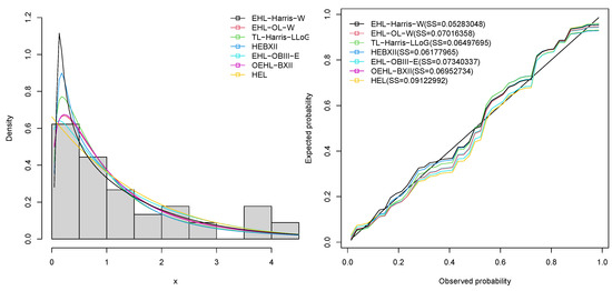
Figure 8. Histogram, fitted density and probability plots for survival times of chemotherapy patients data.

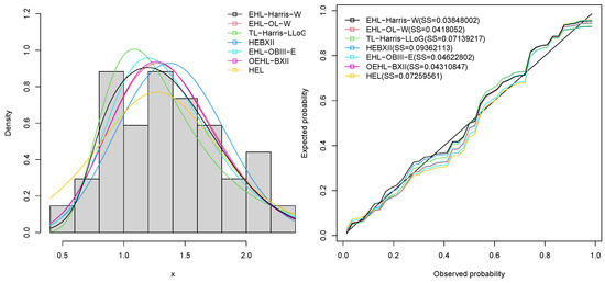
Figure 9. Histogram, fitted density and probability plots for level of mercury data.

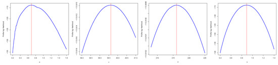
Figure 10. Profile log-likelihood function plots for parameters of EHL-Harris-W distribution on survival times of chemotherapy patients data.

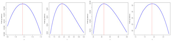
Figure 11. Profile log-likelihood function plots for parameters of EHL-Harris-W distribution on level of mercury data.

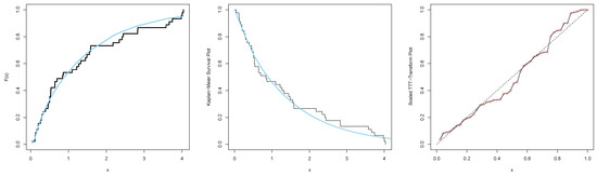
Figure 12. Estimated cdf, Kaplan–Meier survival and scaled TTT–Transform plots for the EHL-Harris-W distribution for survival times of chemotherapy patients data.

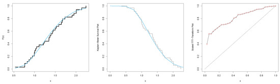
Figure 13. Estimated cdf, Kaplan–Meier survival and scaled TTT–Transform plots for the EHL-Harris-W distribution for level of mercury data.

8.1. Survival Times of Chemotherapy Patients Data

The first data set was a subset of the data reported by [34,35], and it corresponded to the survival times (in years) of a group of 46 patients who received chemotherapy alone. This example was chosen due to the critical importance of survival analysis in medical research and clinical trials. This application can aid in the making of informed decisions about treatment protocols, identifying high-risk patient groups, and evaluating the effectiveness of different therapeutic strategies. The observations were as follows: 0.047, 0.115, 0.121, 0.132, 0.164, 0.197, 0.203, 0.260, 0.282, 0.296, 0.334, 0.395, 0.458, 0.466, 0.501, 0.507, 0.529, 0.534, 0.540, 0.641, 0.644, 0.696, 0.841, 0.863, 1.099, 1.219, 1.271, 1.326, 1.447, 1.485, 1.553, 1.581, 1.589, 2.178, 2.343, 2.416, 2.444, 2.825, 2.830, 3.578, 3.658, 3.743, 3.978, 4.003, 4.033. The estimated variance–covariance matrix for the EHL-Harris-W model on survival times of chemotherapy patients data is given by:

$$\left(\begin{array}{cccc}0.01743& 1.24218& -0.03390& 0.00045\\ 1.24218& 326.73597& -8.91823& 1.13107\\ -0.03390& -8.91823& 0.24342& -0.03087\\ 0.00045& 1.13107& -0.03087& 0.01072\end{array}\right),$$

and the 95% two-sided asymptotic confidence intervals for $\alpha ,v,\delta$ and $\lambda$ are given by $0.6886\pm 0.2587,39.6139\pm 35.4286,216.05\pm 0.9671,$ and $0.8904\pm 0.2031$, respectively.

Table 6 indicates that the EHL-Harris-W distribution had the highest p-value for the K–S statistic and the lowest values for all the goodness-of-fit statistics. Thus, we concluded that the EHL-Harris-W model performed better on the survival times of chemotherapy patients data than the non-nested EHL-OL-W, TL-Harris-LLoG, HEBXII, EHL-OBIII-E, OEHL-BXII and HEL models. Further, Figure 8 shows that our model outperformed the competing non-nested models. Figure 10 shows the profile log-likelihood plots for parameters of the EHL-Harris-W distribution on survival times of chemotherapy patients data. This shows that the MLEs of the EHL-Harris-W distribution can be uniquely determined.

In Figure 12, we see that the cdf line for the EHL-Harris-W distribution, indicated by the blue line, was closer to the empirical cdf, while the survival function in blue was also close to the Kaplan–Meier (K–M) curve, which indicated that our model was the best in explaining the survival times of chemotherapy patients data. The TTT plot for survival times of chemotherapy patients data indicated a non-monotonic hazard rate function; hence, the survival times of chemotherapy patients data can be fitted to our model.

8.2. Level of Mercury Data

The second data set refers to the level of mercury in 34 albacore caught in the Eastern Mediterranean, obtained from [36]. The level of mercury in seafood is an important concern, as it can have adverse effects on human health; particularly, for pregnant women and young children. Therefore, accurately modeling and understanding the distribution of mercury levels can provide valuable information for policymakers and public health officials to make informed decisions regarding fish consumption guidelines and seafood safety regulations. The observations were as follows: 1.007, 1.447, 0.763, 2.010, 1.346, 1.243, 1.586, 0.821, 1.735, 1.396, 1.109, 0.993, 2.007, 1.373, 2.242, 1.647, 1.350, 0.948, 1.501, 1.907, 1.952, 0.996, 1.433, 0.866, 1.049, 1.665, 2.139, 0.534, 1.027, 1.678, 1.214, 0.905, 1.525, 0.763.

The estimated variance–covariance matrix for the EHL-Harris-W model on level of mercury data set is given by:

$$\left(\begin{array}{cccc}4.86956\times {10}^{-07}& -5.82615\times {10}^{-04}& 2.05869\times {10}^{-05}& -8.45610\times {10}^{-05}\\ -5.82615\times {10}^{04}& 6.97295\times {10}^{-01}& -2.45918\times {10}^{-02}& 1.03415\times {10}^{-01}\\ 2.05869\times {10}^{-05}& -2.45918\times {10}^{-02}& 8.92561\times {10}^{-04}& -3.58563\times {10}^{-03}\\ -8.456096\times {10}^{-05}& 1.03415\times {10}^{-01}& -3.58563\times {10}^{-03}& 4.64635\times {10}^{-02}\end{array}\right),$$

and the 95% two-sided asymptotic confidence intervals for $\alpha ,v,\delta$ and $\lambda$ are given by $1.1081\pm 0.0014,8.2914\pm 1.6366,45.2701\pm 0.0586,$ and $1.8880\pm 0.4226$, respectively.

Table 7 indicates that the EHL-Harris-W distribution had the highest p-value for the K-S statistic and the lowest values of all the goodness-of-fit statistics. The EHL-Harris-W model, therefore, worked better with the level of mercury data than did the EHL-OL-W, TL-Harris-LLoG, HEBXII, EHL-OBIII-E, OEHL-BXII and HEL models. In addition, Figure 9 shows that our model outperformed the competing non-nested models on the level of mercury data. Figure 11 shows the profile log-likelihood plots for parameters of the EHL-Harris-W distribution on level of mercury data. This shows that the MLEs of the EHL-Harris-W distribution can be uniquely determined.

In Figure 13, we see that the cdf curve for the EHL-Harris-W distribution, indicated in blue, was closer to the empirical cdf, while the survival function, in blue, was also close to the Kaplan–Meier (K–M) curve, which indicated that our model was the best in explaining the level of mercury data. The TTT plot for level of mercury data indicated an increasing hazard rate function; hence, the level of mercury data can be fitted to our model.

9. Concluding Remarks

This paper develops and presents a novel family of generalized distributions, called the Exponentiated Half Logistic-Harris-G (EHL-Harris-G) distribution. The motivation for introducing this generalized family of distributions lies in its ability to overcome the limitations of previous families, enhance flexibility, improve tail behavior, provide better statistical properties and it has applications in several fields. There are several new distributions in the EHL-Harris-G family of distributions that are special cases or sub-models. There is quite a bit of variation in the behavior of the hazard rate functions of the EHL-Harris-G family of distributions for specific baseline cdfs. The moments, distribution of order statistics, and Rényi entropy are also expressed in closed form. A variety of estimation approaches were used to estimate parameters of the EHL-Harris-G family of distributions. These included maximum likelihood estimation, least-squares estimation, weighted least-squares estimation, maximum product spacing estimation, Cramér–von Mises estimation, and Anderson–Darling estimation. Monte Carlo simulations were used to evaluate the consistency properties of the six estimation methods for a special case of the EHL-Harris-G distribution. The simulation results showed that the MLE and WLS methods almost equally allowed us to obtain better estimates of the EHL-Harris-W parameters, with MLE ranked first, followed by WLS and, then, AD. According to the rankings, the CVM method performed the least well. Risk measures and numerical studies of the measures are also presented. Finally, we showed that the EHL-Harris-W distribution is superior to some other equi-parameter non-nested models in the literature by fitting it to two real-life data sets from different disciplines. In the future, we will extend this new family of distributions via bivariate extensions. This extension can be achieved through various methods, including the use of copulas and probability generating functions. Furthermore, obtaining the distributions of the sums, products, and ratios of random variables will be considered. In addition, future research will incorporate Bayesian estimation methods to estimate model parameters, since Bayesian methods can be applied to almost all parametric methods, and are becoming more popular across disciplines.

References

- Marshall, A.; Olkin, I. A new method for adding a parameter to a family of distributions with application to the exponential and Weibull families. Biometrika 1997, 84, 641–652. [Google Scholar] [CrossRef]
- Eugene, N.; Lee, C.; Famoye, F. Beta-normal distribution and its applications. Commun. Stat.-Theory Methods 2002, 31, 497–512. [Google Scholar] [CrossRef]
- Shaw, W.T.; Buckley, I.R. The alchemy of probability distributions: Beyond gram-charlier expansions, and a skew-kurtotic-normal distribution from a rank transmutation map. arXiv 2009, arXiv:0901.0434. [Google Scholar]
- Zografos, K.; Balakhrishnan, N. On families of beta and generalized gamma generated distribution and associated inference. Stat. Methods 2009, 6, 344–362. [Google Scholar] [CrossRef]
- Cordeiro, G.M.; de Castro, M. A new family of generalized distributions. J. Stat. Comput. Simul. 2011, 81, 883–898. [Google Scholar] [CrossRef]
- Cordeiro, G.M.; Ortega, E.M.; da Cunha, D.C. The exponentiated generalized class of distributions. J. Data Sci. 2013, 11, 1–27. [Google Scholar] [CrossRef]
- Alzaatreh, A.; Lee, C.; Famoye, F. A new method for generating families of continuous distributions. Metron 2013, 71, 63–79. [Google Scholar] [CrossRef]
- Torabi, H.; Montazeri, N.H. The logistic-uniform distribution and its applications. Commun. Stat.-Simul. Comput. 2014, 43, 2551–2569. [Google Scholar] [CrossRef]
- Bourguignon, M.; Silva, R.B.; Cordeiro, G.M. The Weibull-G family of probability distributions. J. Data Sci. 2014, 12, 53–68. [Google Scholar] [CrossRef]
- Alizadeh, M.; MirMostafee, S.; Ortega, E.M.; Ramires, T.G.; Cordeiro, G.M. The odd log-logistic logarithmic generated family of distributions with applications in different areas. J. Stat. Distrib. Appl. 2017, 4, 6. [Google Scholar] [CrossRef][Green Version]
- Soliman, A.H.; Elgarhy, M.A.E.; Shakil, M. Type II half logistic family of distributions with applications. Pak. J. Stat. Oper. Res. 2017, 13, 245–264. [Google Scholar] [CrossRef]
- Alizadeh, M.; Lak, F.; Rasekhi, M.; Ramires, T.G.; Yousof, H.M.; Altun, E. The odd log-logistic Topp–Leone G family of distributions: Heteroscedastic regression models and applications. Comput. Stat. 2018, 33, 1217–1244. [Google Scholar] [CrossRef]
- ZeinEldin, R.A.; Haq, M.A.U.; Hashmi, S.; Elsehety, M.; Elgarhy, M. Type II half logistic Kumaraswamy distribution with applications. J. Funct. Spaces 2020, 2020, 1343596. [Google Scholar] [CrossRef]
- Sengweni, W.; Oluyede, B.; Makubate, B. The exponentiated half-logistic odd Lindley-G family of distributions with applications. J. Nonlinear Sci. Appl. 2021, 14, 287–309. [Google Scholar] [CrossRef]
- El-Sherpieny, E.S.A.; Elsehetry, M.M. Type II kumaraswamy half logistic family of distributions with applications to exponential model. Ann. Data Sci. 2019, 6, 1–20. [Google Scholar] [CrossRef]
- Moakofi, T.; Oluyede, B.; Makubate, B. The half logistic log-logistic Weibull distribution: Model, properties and applications. Eurasian Bull. Math. 2022, 4, 186–210. [Google Scholar]
- Alghamdi, S.M.; Shrahili, M.; Hassan, A.S.; Gemeay, A.M.; Elbatal, I.; Elgarhy, M. Statistical inference of the half logistic modified Kies exponential model with modeling to engineering data. Symmetry 2023, 15, 586. [Google Scholar] [CrossRef]
- Azzalini, A. A class of distributions which includes the normal ones. Scand. J. Stat. 1985, 12, 171–178. [Google Scholar]
- Barakat, H.M. A new method for adding two parameters to a family of distributions with application to the normal and exponential families. Stat. Methods Appl. 2015, 24, 359–372. [Google Scholar] [CrossRef]
- Barakat, H.M.; Khaled, O.M. Towards the establishment of a family of distributions that best fits any data set. Commun. Stat. Simul. Comput. 2017, 46, 6129–6143. [Google Scholar] [CrossRef]
- AL-Hussaini, E.K.; Abdel-Hamid, A.H. Generation of Distribution Functions: A Survey. J. Stat. Appl. Probab. 2018, 7, 91–103. [Google Scholar] [CrossRef]
- Cordeiro, G.M.; Alizadeh, M.; Ortega, E.M. The exponentiated half-logistic family of distributions: Properties and applications. J. Probab. Stat. 2014, 2014, 864396. [Google Scholar] [CrossRef]
- Pinho, L.G.B.; Cordeiro, G.M.; Nobre, J.S. On the Harris-G class of distributions: General results and application. Braz. J. Probab. Stat. 2015, 29, 813–832. [Google Scholar] [CrossRef]
- Dutta, K.; Perry, J. A Tale of Tails: An Empirical Analysis of Loss Distribution Models for Estimating Operational Risk Capital (No. 06-13); Working Papers; Econstor: Singapore, 2006. [Google Scholar]
- Swain, J.J.; Venkatraman, S.; Wilson, J.R. Least-squares estimation of distribution functions in Johnson’s translation system. J. Stat. Comput. Simul. 1988, 29, 271–297. [Google Scholar] [CrossRef]
- Cheng, R.C.H.; Amin, N.A.K. Maximum Product-of-Spacings Estimation with Applications to the Log-Normal Distribution; Mathematical Report 79-1; University of Wales IST: Cardiff, Wales, 1979. [Google Scholar]
- Benkhelifa, L. Alpha power Topp-Leone Weibull distribution: Properties, characterizations, regression modeling and applications. J. Stat. Manag. Syst. 2022, 25, 1–26. [Google Scholar] [CrossRef]
- Teamah, A.E.A.; Elbanna, A.A.; Gemeay, A.M. Heavy-tailed log-logistic distribution: Properties, risk measures and applications. Stat. Optim. Inf. Comput. 2021, 9, 910–941. [Google Scholar] [CrossRef]
- Chen, G.; Balakrishnan, N. A general purpose approximate goodness-of-fit test. J. Qual. Technol. 1995, 27, 154–161. [Google Scholar] [CrossRef]
- Oluyede, B.; Dingalo, N.; Chipepa, F. The Topp-Leone-Harris-G family of distributions with applications. Int. J. Math. Oper. Res. 2023, 24, 554–582. [Google Scholar] [CrossRef]
- Batsidis, A.; Lemonte, A.J. On the Harris extended family of distributions. Statistics 2015, 49, 1400–1421. [Google Scholar] [CrossRef]
- Oluyede, B.; Peter, P.O.; Ndwapi, N.; Bindele, H. The exponentiated half-logistic odd Burr III-G: Model, properties and applications. Pak. J. Stat. Oper. Res. 2022, 18, 33–57. [Google Scholar] [CrossRef]
- Aldahlan, M.; Afify, A.Z. The odd exponentiated half-logistic Burr XII distribution. Pak. J. Stat. Oper. Res. 2018, XIV, 305–317. [Google Scholar] [CrossRef]
- Bekker, A.; Roux, J.J.J.; Mosteit, P.J. A generalization of the compound Rayleigh distribution: Using a Bayesian method on cancer survival times. Commun. Stat.-Theory Methods 2000, 29, 1419–1433. [Google Scholar] [CrossRef]
- Stablein, D.M.; Carter, W.H., Jr.; Novak, J.W. Analysis of survival data with non-proportional hazard functions. Control. Clin. Trials 1981, 2, 149–159. [Google Scholar] [CrossRef] [PubMed]
- Mol, S.; Ozden, O.; Karakulak, S. Levels of selected metals in albacore (Thunnus alalunga, Bonnaterre, 1788) from the Eastern Mediterranean. J. Aquat. Food Prod. Technol. 2012, 21, 111–117. [Google Scholar] [CrossRef]
Disclaimer/Publisher’s Note: The statements, opinions and data contained in all publications are solely those of the individual author(s) and contributor(s) and not of MDPI and/or the editor(s). MDPI and/or the editor(s) disclaim responsibility for any injury to people or property resulting from any ideas, methods, instructions or products referred to in the content. |
© 2023 by the authors. Licensee MDPI, Basel, Switzerland. This article is an open access article distributed under the terms and conditions of the Creative Commons Attribution (CC BY) license (https://creativecommons.org/licenses/by/4.0/).