Communication

On the Extreme Value H-Function

by
Pushpa Narayan Rathie
1,
Luan Carlos de Sena Monteiro Ozelim
2,*,
Felipe Quintino
1 and
Tiago A. da Fonseca
3
1
Department of Statistics, University of Brasilia, Brasília 70.910-900, Brazil
2
Department of Civil and Environmental Engineering, University of Brasilia, Brasília 70.910-900, Brazil
3
Gama Engineering College, University of Brasilia, Brasília 72.444-240, Brazil
*
Author to whom correspondence should be addressed.
Stats 2023, 6(3), 802-811; https://doi.org/10.3390/stats6030051
Submission received: 10 July 2023 / Revised: 2 August 2023 / Accepted: 2 August 2023 / Published: 4 August 2023

Abstract

:
In the present paper, a new special function, the so-called extreme value H -function, is introduced. This new function, which is a generalization of the H-function with a particular set of parameters, appears while dealing with products and quotients of a wide class of extreme value random variables. Some properties, special cases and a series representation are provided. Some statistical applications are also briefly discussed.

1. Introduction and Preliminaries

Special functions have always played a central role in the theory of the algebra of random variables [1]. While dealing with analytical expressions involving certain types of random variables, it is not unusual to face situations where known functions are not capable of providing closed-form expressions for the operations under consideration. Thus, new special functions need to be defined.
When dealing with extreme value random variables, a certain class of integrals appears quite frequently, making it interesting to define a new special function, the so-called extreme value H -function.
As will be demonstrated, the extreme value H -function is a generalization of the H-function with specific parameters. Thus, it is important to first introduce the H-function as the following contour complex integral [2]:
H p , q m , n z | ( a 1 , A ) , , ( a n , A n ) , ( a n + 1 , A n + 1 ) , , ( a p , A p ) ( b 1 , B 1 ) , , ( b m , B m ) , ( b m + 1 , B m + 1 ) , , ( b q , B q ) = 1 2 π i L h ( s ) z s d s ,
where
h ( s ) = j = 1 m Γ ( b j + B j s ) j = 1 n Γ ( 1 a j A j s ) j = m + 1 q Γ ( 1 b j B j s ) j = n + 1 p Γ ( a j + A j s )
with p, q, m, and n are integers such that 0 m q and 0 n p , A j and B j are positive real quantities and all the a j and b j are complex numbers. The contour L runs from c i c + i such that the poles of Γ ( b j + B j s ) , j = 1 , , m lie to the left of L and the poles of Γ ( 1 a j A j s ) , j = 1 , , n lie to the right of L.
Several functions are special cases of the H-function. For example, the generalized hypergeometric series p F q , MacRobert’s E-function, the generalized Bessel–Maitland function, the Krätzel function, the Wright generalized hypergeometric function, Bessel functions, the Whittaker function, the Mittag–Leffler function, trigonometric functions, exponentials and so on [2]. Several authors have studied the properties and generalizations of such hypergeometric functions, such as [3,4,5,6,7,8].
As indicated, the paper is devoted to the definition of the extreme value H -function and is organized as follows: Section 2 introduces the extreme value H -function. Section 3 presents the relationship between the new function and generalized hypergeometric functions. Section 4 indicates a few special cases of the new function, which include the Gamma function and the Krätzel function. In Section 6, statistical applications regarding the products and quotients of extreme value random variables are discussed. Finally, Section 7 presents the conclusions of the present work.

2. The Extreme Value H -Function

Let us consider the extreme-value H -function. This function, hereby denoted as H , can be defined as
H ( a 1 , a 2 , a 3 , a 4 , a 5 , a 6 ) : = 0 y a 6 exp { a 1 y ( a 2 y a 3 + a 4 ) a 5 } d y ,
where ( a 1 ) , ( a 2 ) , ( a 4 ) R + , a 3 , a 5 C . Both ( a 1 ) and ( a 2 ) cannot be equal to zero at the same time. ( a 6 ) > 1 when a 1 0 or a 1 = 0 and sign ( a 3 ) = sign ( a 5 ) , ( a 6 ) < 1 when a 1 = 0 and sign ( a 3 ) sign ( a 5 ) . In this paper, R , C and denote the real numbers, complex numbers and the real part of a complex number, respectively.

General Behavior

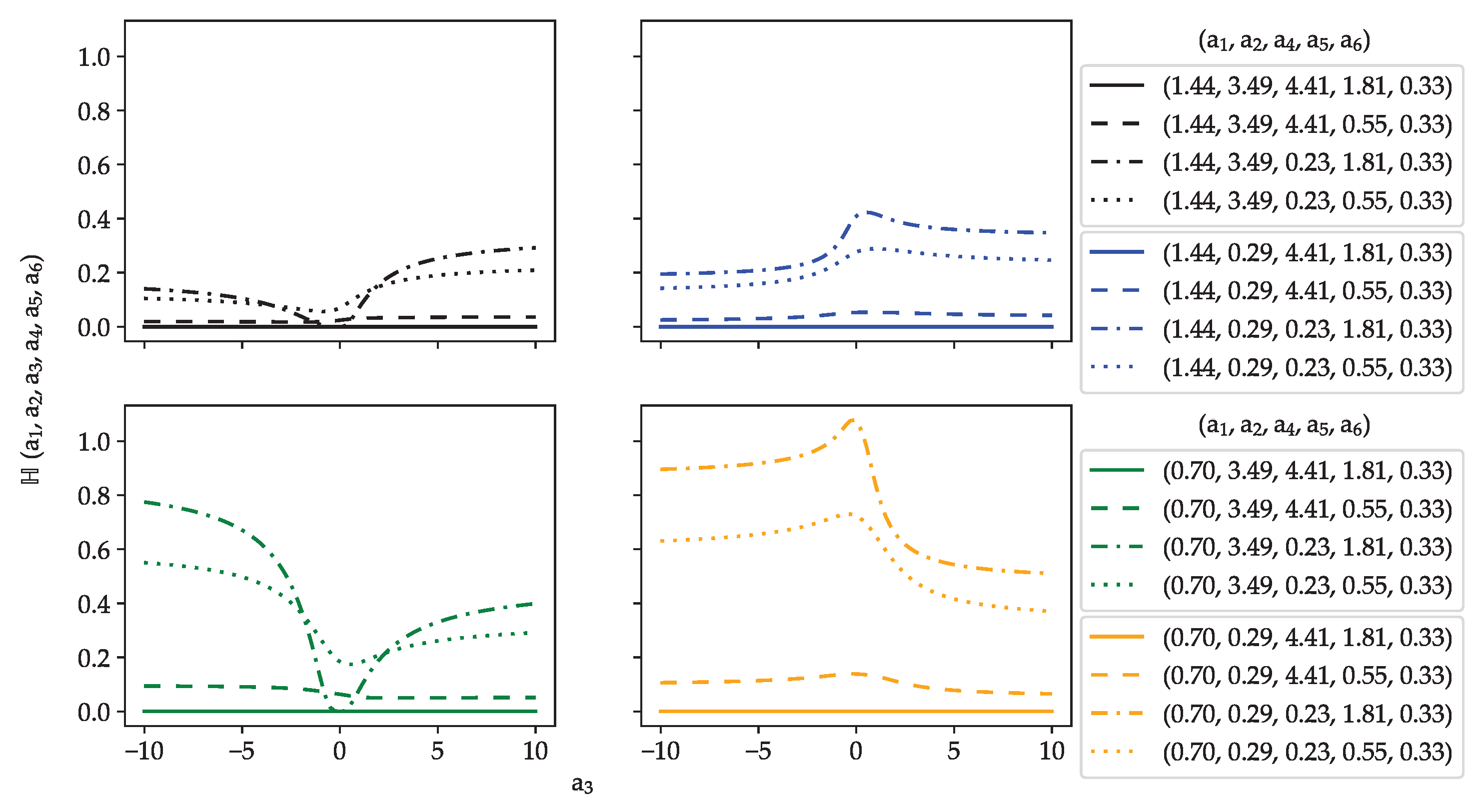
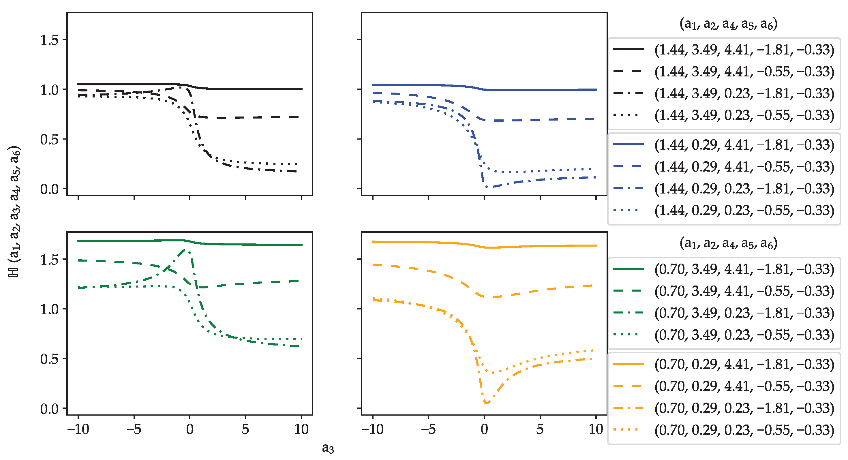
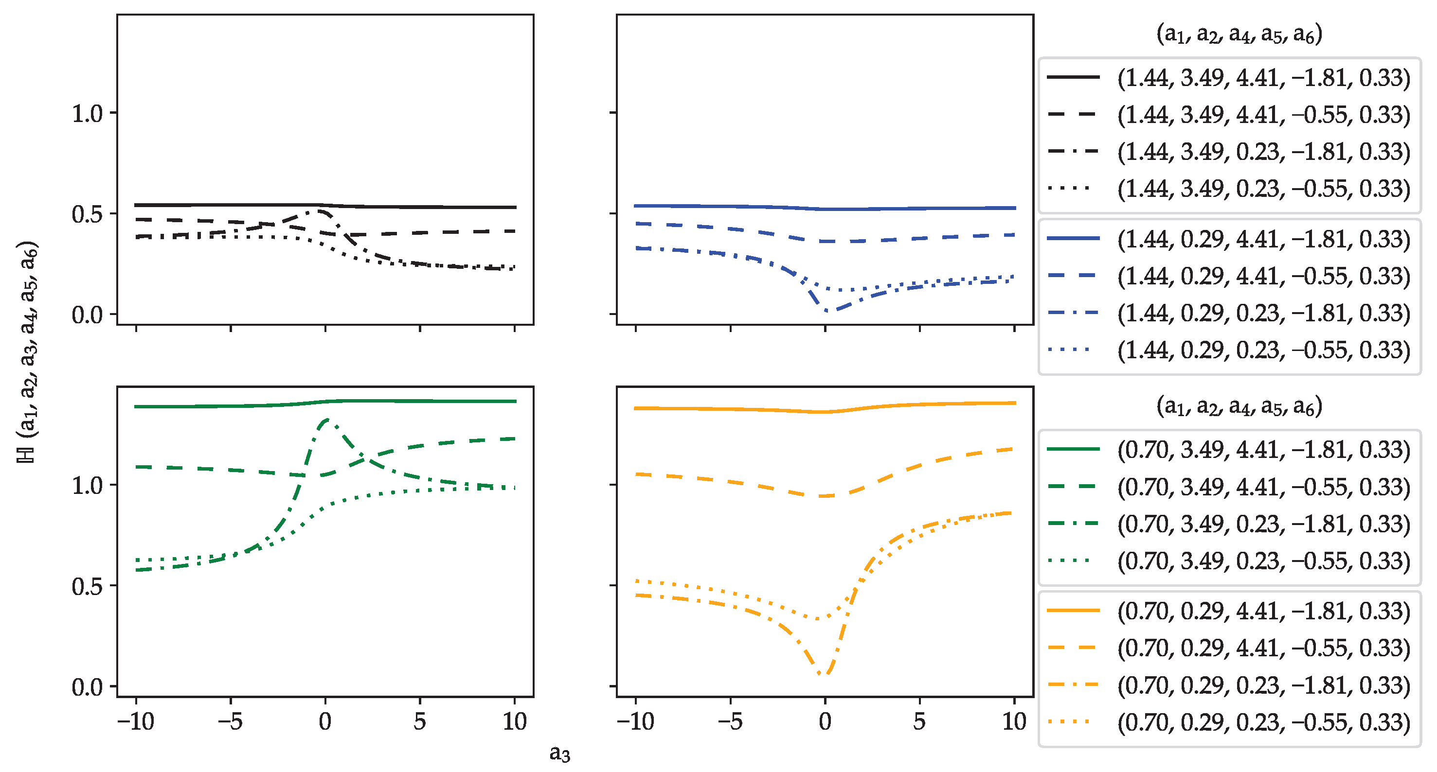
Figure 1, Figure 2, Figure 3 and Figure 4 graphically present the behavior of the new special function whenever its parameters are real numbers. For the non-negative parameters a 1 , a 2 and a 4 , we chose to plot two general cases, 0 < a i 1 and a i > 1 , i = 1 , 2 , 4 , to check how the function behaves in those cases. For parameters a 3 and a 5 , which are defined on the real line, we considered both negative and positive values. For the parameter a 6 , we chose values in the range of ( 1 , 0 ] and also ( 0 , ) .
Overall, it is possible to see that the new function is quite flexible, being able to represent skewed, monotone and non-monotone functions. It is also possible to see that, in general, for the parameters which can be either positive or negative, there is no clear indication of symmetry between cases.

3. Relationship between the Extreme Value H -Function and the H-Function

From the definition in (3), when a 1 > 0 , since 0 < e z 1 for z 0 and by noticing that a 4 0 , it is easy to see that
0 < H ( a 1 , a 2 , a 3 , a 4 , a 5 , a 6 ) H ( a 1 , a 2 , a 3 , 0 , a 5 , a 6 ) Γ ( a 6 + 1 ) a 1 a 6 + 1 , if a 5 0
and
Γ ( a 6 + 1 ) a 1 a 6 + 1 H ( a 1 , a 2 , a 3 , a 4 , a 5 , a 6 ) H ( a 1 , a 2 , a 3 , 0 , a 5 , a 6 ) > 0 , otherwise .
This way, an important special case of this function is obtained by taking a 4 = 0 , which represents an upper (or lower) bound for its value depending on the sign of a 5 . This case is, therefore, an extreme value of the function and can be written in terms of (2) as
H ( a 1 , a 2 , a 3 , 0 , a 5 , a 6 ) = 0 y a 6 exp { a 1 y a 2 a 5 y a 3 a 5 } d y
= 1 a 2 ( 1 + a 6 ) / a 3 a 3 a 5 H 1 , 1 1 , 1 a 1 a 2 1 / a 3 | ( 1 ( 1 + a 6 ) a 3 a 5 , 1 a 3 a 5 ) ( 0 , 1 )
= 1 a 1 a 6 + 1 H 1 , 1 1 , 1 a 2 a 1 a 3 a 5 | ( a 6 , a 3 a 5 ) ( 0 , 1 ) ,
when sign ( a 3 ) = sign ( a 5 ) and
H ( a 1 , a 2 , a 3 , 0 , a 5 , a 6 ) = 1 a 2 ( 1 + a 6 ) / a 3 | a 3 a 5 | H 0 , 2 2 , 0 a 1 a 2 1 / a 3 | ( 0 , 1 ) , ( ( 1 + a 6 ) a 3 a 5 , 1 | a 3 a 5 | )
= 1 a 1 a 6 + 1 H 0 , 2 2 , 0 a 2 a 1 a 3 a 5 | ( 0 , 1 ) , ( 1 + a 6 , | a 3 a 5 | ) ,
otherwise. Both Equations (4) and (5) follow directly from the contour integral definition of the H-function given in (1) and the contour integral representation of the exponential function given as [2]
exp ( z ) = 1 2 π i L Γ ( s ) z s d s

Relationship between the Extreme Value H -Function and Higher-Level Hypergeometric Functions

If one seeks to relate the extreme value H -function to higher-level hypergeometric functions, it is possible to establish a relationship between the new function and the H-function of two variables.
In that case, from Equations (3) and (6):
H ( a 1 , a 2 , a 3 , a 4 , a 5 , a 6 ) = 1 2 π i 0 y a 6 e a 1 y L 1 Γ ( s ) ( a 2 y a 3 + a 4 ) a 5 s d s d y ,
where L 1 is a suitable contour such that ( s ) > 0 . On the other hand, it is known that [2]
( 1 + z ) a = 1 Γ ( a ) H 1 , 1 1 , 1 z | ( 1 a , 1 ) ( 0 , 1 ) , ( a ) > 0 ,
Thus, the combination of Equations (7) and (8) leads to
H ( a 1 , a 2 , a 3 , a 4 , a 5 , a 6 ) = 1 2 π i 0 y a 6 e a 1 y L 1 Γ ( s ) a 4 a 5 s a 2 a 4 y a 3 + 1 a 5 s d s d y = 1 2 π i 0 y a 6 e a 1 y L 1 Γ ( s ) a 4 a 5 s Γ ( a 5 s ) × × H 1 , 1 1 , 1 a 2 a 4 y a 3 | ( 1 a 5 s , 1 ) ( 0 , 1 ) d s d y
whenever a 5 R + .
By using the H-function contour integral representation in (1), the following holds:
H ( a 1 , a 2 , a 3 , a 4 , a 5 , a 6 ) = 1 4 π 2 L 1 L 2 Γ ( s ) Γ ( w ) Γ ( a 5 s + w ) Γ ( a 5 s ) a 4 a 5 s a 2 a 4 w × × 0 y a 6 + a 3 w e a 1 y d y d w d s = 1 4 π 2 L 1 L 2 Γ ( s ) Γ ( w ) Γ ( a 5 s + w ) Γ ( a 5 s ) a 4 a 5 s a 2 a 4 w × × Γ ( a 6 + a 3 w + 1 ) 1 a 1 a 6 + a 3 w + 1 d w d s ,
where L 2 is a suitable contour such that a 5 ( s ) < ( w ) < 0 and ( a 6 + a 3 w + 1 ) > 1 due to the integral performed in the second line of Equation (8). When a 3 R 0 , two possible scenarios occur:
  • a 3 R + : The second inequality indicates that ( w ) > ( 2 + ( a 6 ) ) / a 3 . By combining this result with the limitation that a 5 ( s ) < ( w ) < 0 , it is easy to see that as long as ( s ) > ( 2 + ( a 6 ) ) a 3 1 a 5 1 , both inequalities are satisfied.
  • a 3 R : The second inequality indicates that ( w ) < ( 2 + ( a 6 ) ) / | a 3 | , which implies that by simply taking ( s ) > 0 and a 5 ( s ) < ( w ) < 0 , all inequalities are satisfied.
Thus, whenever a 5 R + and a 3 R 0 , by considering the definition of the H-function of two variables presented in [2] (Definition 2.7), the extreme value H -function can be expressed as
H ( a 1 , a 2 , a 3 , a 4 , a 5 , a 6 ) = 1 a 1 a 6 + 1 H 1 , 0 : 1 , 1 ; 1 , 1 0 , 1 : 0 , 1 ; 1 , 1 a 4 a 5 a 2 a 1 a 3 a 4 1 | ( 1 ; a 5 , 1 ) : ( 1 , 1 ) ; ( a 6 , a 3 ) : ( 1 , a 5 ) ; ( 0 , 1 )
where H 1 , 0 : 1 , 1 ; 1 , 1 0 , 1 : 0 , 1 ; 1 , 1 [ . ] represents the H-function of two variables [2].

4. Special Cases

In Section 3, it is possible to see that a direct special case of the extreme value H -function is the H-function with particular parameters. There are also other special cases which involve H-functions, such as
  • H-function
Let a 5 = 1 , and then
H ( a 1 , a 2 , a 3 , a 4 , 1 , a 6 ) = e a 4 H ( a 1 , a 2 , a 3 , 0 , 1 , a 6 ) ,
Also, let a 5 = 2 and a 3 = 1 , and then
H ( a 1 , a 2 , 1 , a 4 , 2 , a 6 ) = e a 4 2 H ( a 1 + 2 a 2 a 4 , a 2 , 1 , 0 , 2 , a 6 ) ,
where H ( a 1 , a 2 , a 3 , 0 , a 5 , a 6 ) is presented in Equations (4) and (5).
A sub-case of the H-function cases is related to the Krätzel function, defined as [9]
Z ρ ν ( x ) = 0 t ν 1 exp t ρ x / t d t ,
when x > 0 , ρ R and ν C , being such that ( ν ) < 0 when ρ 0 .
Thus, a direct consequence of (5) is that
H ( x , 1 , ρ , 0 , 1 , 1 ν ) = Z ρ ν ( x ) ,
when ( ν ) < 0 and ρ 0 . Also, when ρ > 0 and ( ν ) > 0 ,
H ( 1 , x , ρ 1 , 0 , 1 , ν / ρ 1 ) = ρ Z ρ ν ( x ) .
Other special and ordinary functions also show up as special cases, namely
  • Gamma function
Let a 2 = 0 , and then
H ( a 1 , 0 , a 3 , a 4 , a 5 , a 6 ) = Γ ( a 6 + 1 ) a 1 a 6 + 1 e a 4 a 5
On the other hand, let a 5 = 0 , and then
H ( a 1 , a 2 , a 3 , a 4 , 0 , a 6 ) = Γ ( a 6 + 1 ) a 1 a 6 + 1
It is also possible to express the extreme value H -function when a 5 is a natural number m as an infinite series of Gamma functions. In such cases, let us assume that a 1 > 0 :
H ( a 1 , a 2 , a 3 , a 4 , m , a 6 ) = 1 a 1 a 6 + 1 n = 0 ( a 4 m ) n n ! k = 0 m n ( m n ) ! ( m n k ) ! k ! a 2 a 4 a 1 a 3 k Γ ( a 6 + 1 + a 3 k ) ,
which is a consequence of expanding the exponential function into a power series and then applying the binomial theorem.

5. Series Representation

Let us consider the following general integral, such that α > 1 is a real number:
0 x α e x f ( x ) d x .
By considering the generalized Gauss–Laguerre quadrature, it is possible to approximate (17) by [10]:
0 x α e x f ( x ) d x i = 1 n w i , α f ( x i ) ,
where x i is the i-th root of the generalized Laguerre polynomials L n ( α ) ( x ) and the weight w i , α is given by [10,11]:
w i , α = Γ ( n + α + 1 ) x i n ! ( n + 1 ) 2 [ L n + 1 ( α ) ( x i ) ] 2
and with error term E n given as [11]:
E n = n ! Γ ( n + α + 1 ) ( 2 n ) ! f ( 2 n ) ( ξ ) ,
where ξ is in the domain of f ( x ) . Equation (20) reveals that the quadrature is exact whenever f ( x ) is a polynomial of up to 2 n 1 order.
This way, from Equations (3) and (18), a computable representation of the extreme value H -function, when a 1 > 0 and a 2 0 , is
H ( a 1 , a 2 , a 3 , a 4 , a 5 , a 6 ) 1 a 1 1 + a 6 i = 1 n w i , a 6 exp { ( a 2 a 1 a 3 x i a 3 + a 4 ) a 5 } ,
which is a fast converging series due to the exponential nature of its terms. The series can be made as accurate as needed by increasing the number of terms taken. On the other hand, when a 2 > 0 and a 1 = 0 ,
H ( 0 , a 2 , a 3 , a 4 , a 5 , a 6 ) i = 1 n w i , a 6 exp { ( a 2 x i a 3 + a 4 ) a 5 + x i } ,
which is a direct consequence of Equation (17) when f ( x ) = e x g ( x ) .

6. Applications to Extreme Value Statistical Theory

At first glance, an interesting characteristic of the extreme value H -function is that it is always non-negative and bounded. This suggests it could be used as a normalizing constant for a probability density function (pdf) given by its integrand. In this case, let X be a positive random variable whose probability density function g ( x ) is given in terms of the parameters ( a 1 , a 2 , a 3 , a 4 , a 5 , a 6 ) as
g ( x ) = c 1 x a 6 exp { a 1 x ( a 2 x a 3 + a 4 ) a 5 } x 0 ,
where c is a normalizing constant to make the integral of g ( x ) be equal to 1 along its full support. Then, it is clear that c = H ( a 1 , a 2 , a 3 , a 4 , a 5 , a 6 ) whenever the constants a 1 , a 2 , a 3 , a 4 , a 5 , and a 6 follow the restrictions indicated in the definition of H .
By using the extreme value H -function, a number of important characteristics of the random variable X can be described, such as its complex moments. In that case, the Mellin transform { M g } ( s ) of g ( x ) is given as
{ M g } ( s ) = c 1 0 y s 1 + a 6 exp { a 1 y ( a 2 y a 3 + a 4 ) a 5 } d y = H ( a 1 , a 2 , a 3 , a 4 , a 5 , s 1 + a 6 ) H ( a 1 , a 2 , a 3 , a 4 , a 5 , a 6 ) .
It is known that the Mellin transform is important in determining the distributions of the products and quotients of independent random variables [1,12]. In those cases, the convolution property of the Mellin transform indicates the following: Let A and B be independent random variables whose pdfs a ( x ) and b ( x ) are given as in Equation (23) with parameters a 1 , a 2 , a 3 , a 4 , a 5 , and a 6 and b 1 , b 2 , b 3 , b 4 , b 5 , and b 6 , respectively. Then, assume one wants to find the pdf p ( x ) of the random variable P = A B . Then,
{ M p } ( s ) = { M a } ( s ) { M b } ( s ) .
On the other hand, let Q = A / B with pdf q ( x ) . Assuming the independence of A and B, it is possible to state that
{ M q } ( s ) = { M a } ( s ) { M b } ( 2 s ) .
One may refer to [1] for further details on the properties of Mellin transforms in the context of the algebra of random variables.
Thus, it is possible to see that, by combining Equations (24)–(26), the densities of products and quotients of random variables whose pdfs are of the form (23) can be readily given in terms of the extreme value H -function by an inverse Mellin transform. This way,
p ( x ) = 1 2 π i L x s H ( a 1 , a 2 , a 3 , a 4 , a 5 , s 1 + a 6 ) H ( a 1 , a 2 , a 3 , a 4 , a 5 , a 6 ) H ( b 1 , b 2 , b 3 , b 4 , b 5 , s 1 + b 6 ) H ( b 1 , b 2 , b 3 , b 4 , b 5 , b 6 ) d s
and
q ( x ) = 1 2 π i L * x s H ( a 1 , a 2 , a 3 , a 4 , a 5 , s 1 + a 6 ) H ( a 1 , a 2 , a 3 , a 4 , a 5 , a 6 ) H ( b 1 , b 2 , b 3 , b 4 , b 5 , 1 s + b 6 ) H ( b 1 , b 2 , b 3 , b 4 , b 5 , b 6 ) d s
where L and L * are suitable contours (line integral taken over a vertical line in the complex plane), whose validity conditions are given in the Mellin inversion theorem [1,2].
Not only products and quotients can be given in terms of the extreme value H -function, but also reliability measures of the type P ( A < B ) , when both A and B have their pdfs given as in (23). It is easy to see that for positive random variables A and B, P ( A < B ) = P ( A / B < 1 ) ; therefore, the density of the random variable Q = A / B is pivotal to obtain P ( A / B < 1 ) . Thus, from (28),
P ( A < B ) = 0 1 q ( x ) d x
= 1 2 π i L * H ( a 1 , a 2 , a 3 , a 4 , a 5 , s 1 + a 6 ) H ( a 1 , a 2 , a 3 , a 4 , a 5 , a 6 ) ×
× H ( b 1 , b 2 , b 3 , b 4 , b 5 , 1 s + b 6 ) H ( b 1 , b 2 , b 3 , b 4 , b 5 , b 6 ) 1 1 s 1 s d s ,
whenever ( s ) < 1 . A few distributions whose pdfs are special cases of (23) are as follows: Exponential, Weibull, Rayleigh, Nakagami-m, Generalized Gamma, Half-Normal, Fréchet and some p-max stable distributions [13]. As can be seen, most of the special cases can be related to extreme distributions, which led to the naming of the new function as the extreme value H -function. Table 1 presents the particular values of a i (and, therefore, b i ), i = 1 , . . . , 6 , which would result in the special cases mentioned. In the case of the Fréchet distribution, a variable change can be made in the integral to make the parameters follow the restrictions in (3).

7. Conclusions

New special functions are needed whenever certain analytical calculations are made easier by a compact representation of a given integrand. In the present paper, while dealing with independent extreme distributions, their products, quotients, and reliability measures of the type P ( X < Y ) can all be given in terms of a particular integral, hereby named the extreme value H -function.
This new function is quite flexible, being able to represent skewed, monotone and non-monotone functions. It is also possible to see that, in general, for the parameters which can be either positive or negative, there is no clear indication of symmetry between cases.
A general computable form in terms of series of exponential functions has been presented. Furthermore, other special functions have been shown to be particular cases of the new function, namely the Gamma function, Krätzel function, and H-function. These cases, together with the statistical applications presented, show the wide applicability of the new function. While compared to even higher-level hypergeometric functions, it has been shown that if some parameters are taken as subsets of the real line (positive non-null reals and non-null real numbers, specifically), which is the case of the statistical applications considered, the extreme value H -function can be expressed as a H-function of two variables. This new representation may be useful if further generalizations are envisioned.
Future work may explore other special cases as well as the general behavior of the probability density function defined as the integrand of the new special function. Obtaining random numbers from this distribution may also be of interest. Finally, more general reliability measures of the so-called s out of k stresses system (with individual stresses following extreme random variables) subjected to a random strength also following extreme distributions can be analytically investigated using the new special function.

Author Contributions

Conceptualization, L.C.d.S.M.O.; methodology, P.N.R. and L.C.d.S.M.O.; software, L.C.d.S.M.O.; validation, P.N.R., L.C.d.S.M.O. and F.Q.; formal analysis, P.N.R. and L.C.d.S.M.O.; investigation, L.C.d.S.M.O., F.Q. and T.A.d.F.; writing—original draft preparation, L.C.d.S.M.O.; writing—review and editing, P.N.R., F.Q. and T.A.d.F.; supervision, P.N.R. All authors have read and agreed to the published version of the manuscript.

Funding

This research received no external funding and the APC was kindly waived by the Editorial Office of Stats.

Institutional Review Board Statement

Not applicable.

Informed Consent Statement

Not applicable.

Data Availability Statement

Not applicable.

Acknowledgments

The authors acknowledge the support provided by the University of Brasilia (UnB).

Conflicts of Interest

The authors declare no conflict of interest.

References

  1. Springer, M.D. The Algebra of Random Variables; John Wiley: New York, NY, USA, 1979. [Google Scholar]
  2. Mathai, A.M.; Saxena, R.K.; Haubold, H.J. The H-Function: Theory and Applications; Springer: New York, NY, USA, 2010. [Google Scholar]
  3. Dziok, J.; Srivastava, H. Classes of analytic functions associated with the generalized hypergeometric function. Appl. Math. Comput. 1999, 103, 1–13. [Google Scholar] [CrossRef]
  4. Srivastava, H.M.; Agarwal, P.; Jain, S. Generating functions for the generalized Gauss hypergeometric functions. Appl. Math. Comput. 2014, 247, 348–352. [Google Scholar] [CrossRef]
  5. Srivastava, H. Generalized hypergeometric functions with integral parameter differences. Indag. Math. Proc. 1973, 76, 38–40. [Google Scholar] [CrossRef]
  6. Saxena, R.K.; Kumar, R. A basic analogue of the generalized H-function. Le Matematiche 1995, 50, 263–271. [Google Scholar]
  7. Nisar, K.S.; Rahman, G.; Choi, J.; Mubeen, S.; Muhammad, A. Generalized hypergeometric k-functions via (k, s)-fractional calculus. J. Nonlinear Sci. Appl. 2017, 10, 1791–1800. [Google Scholar] [CrossRef] [Green Version]
  8. Nisar, K.S. On the generalized modified k-Bessel functions of the first kind. Commun. Korean Math. Soc. 2017, 32, 909–914. [Google Scholar] [CrossRef]
  9. Kilbas, A.; Saxena, R.K.; Trujillo, J. Krätzel function as a function of hypergeometric type. Fract. Calc. Appl. Anal. 2006, 9, 109–131. [Google Scholar]
  10. Stroud, A.H.S.D. Gaussian Quadrature Formulas (without Numerical Tables); Prentice-Hall Series in Automatic Computation; Prentice-Hall: Hoboken, NJ, USA, 1966. [Google Scholar]
  11. Abramowitz, M.; Stegun, I.A. Handbook of Mathematical Functions with Formulas, Graphs, and Mathematical Tables; Dover: New York, NY, USA, 1964. [Google Scholar]
  12. Epstein, B. Some Applications of the Mellin Transform in Statistics. Ann. Math. Stat. 1948, 19, 370–379. [Google Scholar] [CrossRef]
  13. Christoph, G.; Falk, M. A note on domains of attraction of p-max stable laws. Stat. Probab. Lett. 1996, 28, 279–284. [Google Scholar] [CrossRef]
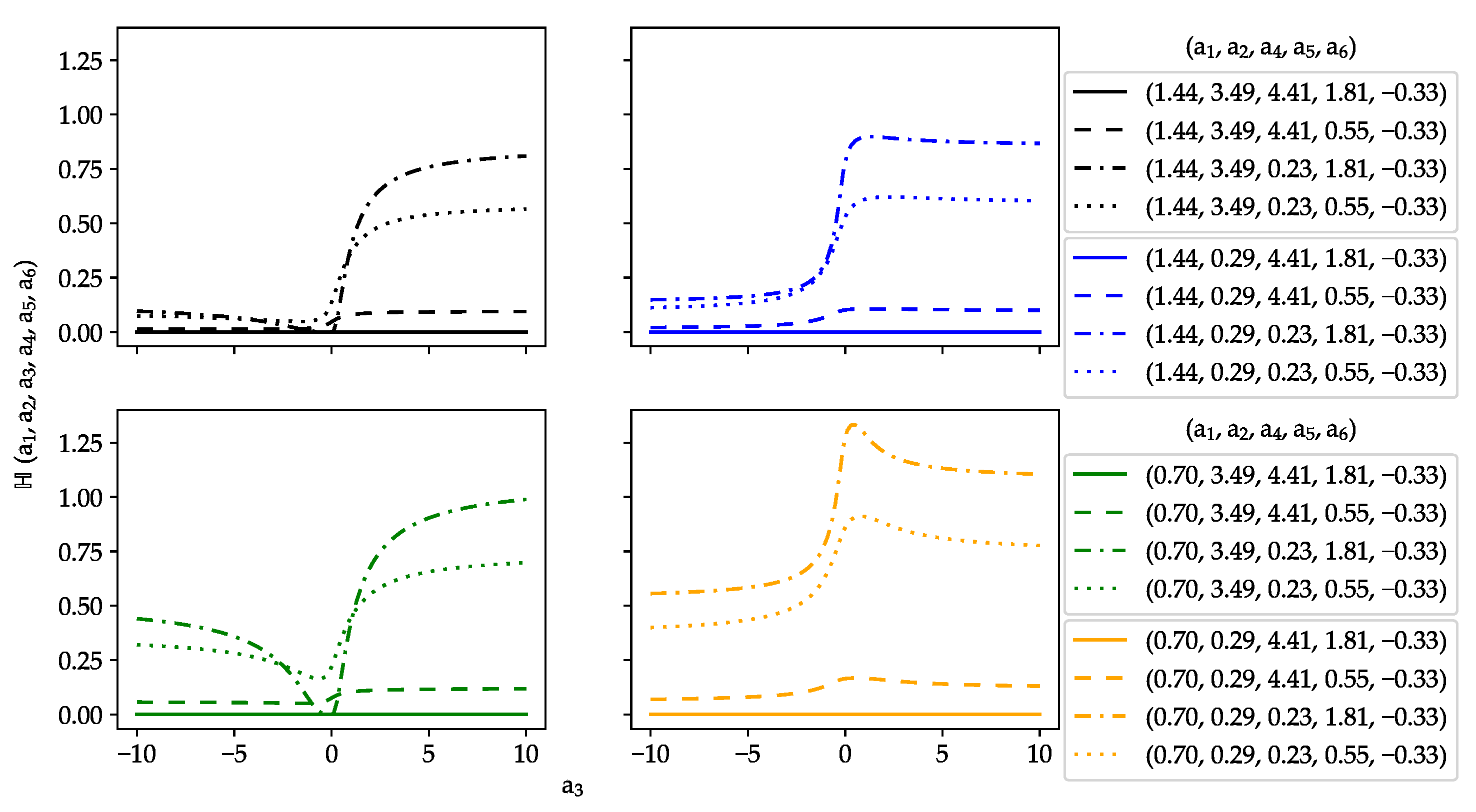
Figure 1. The extreme value H -function for several values of its parameters, with a 5 > 0 and 1 < a 6 < 0 .
Stats 06 00051 g001
Figure 2. The extreme value H -function for several values of its parameters, with a 5 > 0 and a 6 > 0 .
Stats 06 00051 g002
Figure 3. The extreme value H -function for several values of its parameters, with a 5 < 0 and 1 < a 6 < 0 .
Stats 06 00051 g003
Figure 4. The extreme value H -function for several values of its parameters, with a 5 < 0 and a 6 > 0 .
Stats 06 00051 g004
Table 1. Particular values of a i for some special random variable cases. The parameters follow the restrictions in (3).
Random Variable a 1 a 2 a 3 a 4 a 5 a 6
Exponential λ 00000
Weibull0 λ 1 10k k 1
Rayleigh0 ( 2 σ ) 1 1021
Nakagami-m0 ( m / Ω ) 1 / 2 102 2 m 1
Generalized Gamma0 1 / a 10p d 1
Half-Normal0 ( 2 σ ) 1 1020
Fréchet0 1 / s 10 α 1 α
Disclaimer/Publisher’s Note: The statements, opinions and data contained in all publications are solely those of the individual author(s) and contributor(s) and not of MDPI and/or the editor(s). MDPI and/or the editor(s) disclaim responsibility for any injury to people or property resulting from any ideas, methods, instructions or products referred to in the content.