Abstract
In this article, we introduce two new bivariate Kumaraswamy (KW)-type distributions with univariate Kumaraswamy marginals (under certain parametric restrictions) that are less restrictive in nature compared with several other existing bivariate beta and beta-type distributions. Mathematical expressions for the joint and marginal density functions are presented, and properties such as the marginal and conditional distributions, product moments and conditional moments are obtained. Additionally, we show that both the proposed bivariate probability models have positive likelihood ratios dependent on a potential model for fitting positively dependent data in the bivariate domain. The method of maximum likelihood and the method of moments are used to derive the associated estimation procedure. An acceptance and rejection sampling plan to draw random samples from one of the proposed models along with a simulation study are also provided. For illustrative purposes, two real data sets are reanalyzed from different domains to exhibit the applicability of the proposed models in comparison with several other bivariate probability distributions, which are defined on
1. Introduction
In recent years, several articles have demonstrated the applicability of the Kumaraswamy (KW) distribution, and various extensions of univariate KW distributions are also well established in the literature. Extensions to the bivariate and multivariate domains have also received great attention from researchers. There has been growing interest in constructing bivariate and multivariate KW distributions recently. Since the existing bivariate KW distributions cannot adequately fit all types of data, several attempts have been made to construct bivariate KW-type models. A non-exhaustive list of such references are given below. Ref. [1] developed and discussed a bivariate KW distribution based on a minimization strategy. Ref. [2] discussed the construction of a bivariate weighted KW model and provided some structural properties and applications of such a model based on real life data. Ref. [3] discussed some alternative ways of constructing a bivariate KW models via conditional specification, conditional survival specification, Ref. [4] bivariate beta construction, and a strategy based on [5] proposed model with a slight modification. In a separate article, Ref. [6] also discussed the copula based the construction of various types of bivariate KW-type models and discussed the correlation structure and flexibility associated with such models. Noticeably, all the previous work regarding construction of a bivariate KW distribution has one striking similarity, and that is their marginals, as well as the conditionals also being of the KW type with appropriate model parameters. On the contrary, in this paper, we are proposing two arbitrary, absolutely continuous bivariate KW-type models, which under certain restrictions of the model parameters subsume the independent KW models. The proposed probability models have shape parameters that belong to the marginal densities of X and but there are also dependence parameters which involve both the shape and scale parameters, as the case may be. We want to examine whether such types of models under simple linear constraints for the parameters, assuming a known univariate probability model (in our case, a univariate KW), can possess some tractability advantages and fit certain types of data. It appears that both the models have closed-form expressions for moments, with the product moment correlation coefficient involving special functions or series. This is a totally new approach in constructing an absolutely continuous bivariate KW-type distribution. Note that the various types of bivariate KW distributions have led to useful applications in several areas, such as characterizing earthquake data in Turkey [7], the modeling of the proportions of substances in a mixture, brand shares (see [8]) and proportions of elaborate voting for a candidate in a two-candidate election, see [9]. We also argue that these models, including those that are developed in this article, can also be effectively used as priors for the proportion parameter(s) of a bivariate binomial distribution in the context of inference under the Bayesian paradigm.
In this paper, we develop and study two different bivariate, absolutely continuous probability distributions that are defined on a unit square with the property that under independence, based on certain parametric restrictions, both the marginals are univariate KW distributions with suitable shape parameters. We study several useful structural properties such as the shape of the distribution and likelihood ratio dependence for both models. Next, we propose the following two models:
- Model In this case, we assume the joint density will be of the formwhere D is an appropriate normalizing constant which can be obtained throughSome representative plots of the bivariate density for varying parameter choices are given in Appendix A.In this case, the parametric restrictions are the following: , , and . The parameters and influence the correlation measure between the X and Y components of the distribution. Note that when , the joint density reduces to the product of two independent univariate KW random variables, particularly when and independently. Since the KW distribution has two shape parameters, it appears that the marginals of both X and Y have the same second shape parameter, specifically , but different first shape parameters, which are and , respectively. Potential application of such bivariate probability models can be envisioned in real-life scenarios where, for example, X and Y have data structures such that one characteristic is common to both of them, but the other one is different. The only factor that might work as a deterrent regarding the flexibility of such a model is how a practitioner can guarantee that restrictions such as and would be met in reality. Notice that since and one can easily observe that Additional discussion of the parameters is given in the structural properties section later. However, one may consider appropriate testing of the hypothesis as a part of model fitting regarding whether these parametric constraints are met.In the next section, we consider another bivariate KW-type model that we conjecture to have some flexibility in terms of modeling positively dependent data.
- Model Suppose that the joint density is of the formwhere C is an appropriate normalizing constant. Note that when , the joint density reduces to two independent KW random variables with respective parameters.Noticeably, when it appears that and independently. Therefore, by invoking independence via a linear constraint on the parameters, component-wise, the marginals of both X and Y follow a scaled version of a two-parameter univariate KW distribution with the scale factors and , respectively. Furthermore, this model is significantly different from the first proposed model in the sense that we bring in scale factors to capture the variability of X and and the shape parameters are different. This feature is different from the first model, in which the second shape parameter is the same for both X and Once again, as before, a natural objection that might occur in terms of application in modeling real-life data based on this probability model is how our informed expert can guarantee that for dependence modeling, the linear restriction is not satisfied. One simple strategy would be to simply consider a hypothesis test of independence, which can be written as follows:against the alternativeSome additional discussion on the parameters is given in the structural properties section for this model later.
At the outset, we define the following mathematical functions which will be used time and again:
- (1)
- The Gauss hypergeometric function is defined byIn addition, denotes the ascending factorial.
- (2)
- The series expansion is given by
The rest of this paper is organized as follows. In Section 2, we discuss some properties of the first model. Section 3 covers model 2 and the description of some of its structural properties. The associated estimation procedure by the method of maximum likelihood and the method of moments is presented in Section 4 for model In Section 5, we provide a layout of the simulation scheme, assuming that model 1 can be adopted for model 2 as well, and a small simulation study based on model 1 is included. Section 6 deals with two real-life data sets that are reanalyzed to exhibit the applicability of the proposed two models. Finally, some concluding remarks are included in Section 7.
2. Bivariate KW-Type Model 1 Structural Properties
Note that by using the series expansion in Equation (4), one can rewrite the joint density for model 1 given in Equation (1):
2.1. Marginal Densities
The marginal density of Y given from Equation (1) will be
upon using Mathematica and the Gauss hypergeometric function given in Equation (3).
Interpretation of the model parameters:
The four parameters and can be interpreted by examining the behavior of the probability model in Equation (1) near the boundaries of the simplex :
- Observe that as Thus, the distribution of Y along the vertical boundary of the simplex belongs to a univariate KW distribution with two shape parameters: and The parameter represents the scale variation from a standard KW model.
- Likewise, as Therefore, the distribution of X along the vertical boundary of the simplex belongs to a univariate KW distribution with two shape parameters and The parameter represents the scale variation from a standard KW model.
2.2. Conditional Distributions
The conditional density of Y, given , will be
Hence, an expression for the mth-order conditional moment of Y, given (for any ), will be
upon using Mathematica. Similarly, one can find an expression for the conditional density of X given and the corresponding conditional moments.
2.3. Marginal Moments
For any integer (by direct integration using Mathematica), from the marginal density of Y from Equation (8), we have
upon further simplification and using the relationship between the gamma function and the beta function.
Similarly, the marginal mth-order raw moment () of X will be (from the marginal density of X from Equation (7)
after some simplification, as shown before.
2.4. Product Moment
From the joint density expression in Equation (5), and for any non-negative , we have
upon using Mathematica.
The next result represents the closed-form expression for the product moment correlation coefficient:
Corollary 1.
The Pearson’s product moment correlation coefficient of for the bivariate density in Equation (1) will be given by
where
Similarly, we have
Proof.
This immediately follows from Equation (11) by substituting and into Equations (9) and (10), respectively. □
2.5. Distributional Properties
A distribution is said to be positive likelihood ratio-dependent (PLRD) if its p.d.f. satisfies
∀ (see [10] for pertinent details). Next, for the joint p.d.f. in Equation (1), the condition given in Equation (13) is equivalent to , which clearly holds, provided and . This property of being PLRD has several implications that can be associated with the bivariate density in Equation (1), such as the following:
- The bivariate density in Equation (1) is positive regression-dependent (PRD) (i.e.,is decreasing in y for all and similarly, is decreasing in x for all y).
- Furthermore, the property of being PRD will imply that is non-decreasing in x for all y and that is non-increasing in x for all each of which imply that and , namely such that X and Y are positive quadrant-dependent (PQD).
Next, let us consider the shape of the bivariate density given in Equation (1). The derivatives of with respect to x and y are
By setting Equations (14) and (15) to zero, one notes that the critical points for the joint density in Equation (1) are given by the simultaneous solutions of the two equations
Thus, the bivariate density in Equation (1) can exhibit multiple critical points (to be precise, ).
3. Model 2’s Structural Properties
We begin this section by deriving the marginal densities from the bivariate density in Equation (2).
Marginal densities:
First, note that using the binomial expansion, the joint p.d.f. in Equation (2) can be rewritten as
Observe that the sum will stop at if is an integer. From Equation (17), the marginal density of Y can be obtained as follows:
Similarly, the marginal density of X will be
by the same argument as before in writing the joint p.d.f. in an equivalent form.
Interpretation of the model parameters:
The six parameters and can be interpreted by examining the behavior of the probability model in Equation (2) near the boundaries of the simplex :
- Observe that as Thus, the distribution of Y along the vertical boundary of the simplex belongs to a univariate KW distribution with two shape parameters and The parameter represents the scale variation from a standard KW model.
- Likewise, as Thus, the distribution of Y along the vertical boundary of the simplex belongs to a univariate KW distribution with two shape parameters and The parameter represents the scale variation from a standard KW model.
The expressions for the conditional moments cannot be obtained analytically, and numerical integration might be required in this case.
Distributional Properties
For the joint density in Equation (2), the condition in Equation (13) is equivalent to , which clearly holds, provided and . Therefore, the bivariate density in Equation (2) is positive likelihood ratio-dependent (PLRD), which subsequently implies that X and Y are positive quadrant-dependent.
Next, let us consider the shape of the density in Equation (2). The derivatives of with respect to x and y are
Therefore, from Equations (19) and (20), it is evident that the joint p.d.f. in Equation (2) can exhibit several critical points. One may obtain several other useful structural properties, albeit with computational complexity similar to that of the first model discussed earlier.
4. Inference
In this section, we discuss the estimation of the model parameters for the bivariate density given in Equation (1), parameterized by We consider the estimation of the four parameters with the methods of moments and the method of maximum likelihood. The associated Fisher information matrix is available upon request from the author. Suppose that is a random sample drawn from the bivariate density in Equation (1).
4.1. Method of Moments Estimation
However, at first, we consider the method of moments estimators of the four parameters, which can be obtained as the simultaneous solutions of the following equations (upon using the joint moment expression given in Equation (13)):
4.2. Maximum Likelihood Estimation
For the joint density in Equation (1), the associated log-likelihood function can be expressed as
The first-order derivatives of this with respect to the four parameters are
The maximum likelihood estimators of are the simultaneous solutions to Equations (22)–(25), respectively, by setting them individually to zero. For real-data application, it is these MLEs that are considered for the parameter estimation.
5. Simulation
In this section, we consider the simulation from the bivariate density in Equation (1) using an acceptance-rejection algorithm. We note that a similar strategy can be adopted for the bivariate density in Equation (2). Let where D is the normalizing constant. The following scheme may be adopted:
- Generate independent Kumaraswamy random variables U and V with shape parameters and respectively.
- Generate a uniform [0, 1] random variable W independent from
- If , then accept as a realization from the bivariate density in Equation (1).
- If then return to step
We note that there are standard routines for generating independent Kumaraswamy random variables. Next, to illustrate the feasibility of the suggested estimation strategy, a small simulation study was undertaken. The simulation study was carried out for one representative set of parameters for model 1 (Equation (1)), and the process was repeated 15000 times. Three different sample sizes and 300 were considered. The bias (actual estimate) and the standard deviation of the parameter estimates for the maximum likelihood estimates were determined from this simulation study, and they are presented in Table 1 for bivariate probability model 1 in Equation (1).

Table 1.
Bias and standard deviation for the parameters for bivariate probability model 1.
Remark 1.
6. Real Data Application
In this section, we consider two applications of the proposed bivariate weighted Kumaraswamy distribution-based data sets that have been utilized by several other authors as well in the past:
- Data Set I: Earthquakes become major societal risks when they strike vulnerable populations. We consider the data obtained from [7]. Due to the fact that a significant portion of Turkey is subject to frequent earthquakes, destructive mainshocks and their foreshock and aftershock sequences, the area between the longitudes 39 and 42 N and latitudes 26 and 45 E was investigated. In this particular region, 111 mainshocks with surface magnitudes () of five or more occurred in the past 106 years. We define the following random variables. X represents the magnitude of the foreshocks, and Y represents the magnitude of the aftershocks. We fit the data to the following bivariate KW models.
- Data Set II: The data on 45 patients were available from a private clinic in Tennessee regarding the hemoglobin content in blood being prone to type II diabetes. To see the effect of reducing the hemoglobin content in the blood, a special type of treatment was administered to those patients. We define the following variables. X is a random variable which represents the proportion of hemoglobin content in the blood before the treatment, and Y is a random variable which represents the proportion of hemoglobin content in the blood after treatment.
- Model I: Bivariate distribution as defined in Equation (1);
- Model II: Bivariate distribution as defined in Equation (2);
- Model III: Bivariate Kumaraswamy (absolutely continuous distribution, according to [3], in Equation (5));
- Model IV: Bivariate Kumaraswamy distribution via conditional specification, according to [5], given bywhere C is an appropriate normalizing constant;
- Model V: Bivariate Kumaraswamy distribution via conditional survival specification, according to Arnold and Ghosh (2016), given by
- Model VI: [11] bivariate ’s beta distribution, given byfor and where C is the normalizing constant.
- Model VII: [12] bivariate generalized beta distribution given byfor and where C is the normalizing constant.
To verify the efficacy of all four models utilized here, a goodness-of-fit statistic and the AIC and BIC values were computed using the computational package R. The MLEs were computed using the nonlinear optimization package in while for the estimation of parameters for the two newly proposed probability models (as given in Equations (1) and (2)), we considered constrOptim in In addition, regarding fitting of the marginal densities of X and Y, as suggested by one reviewer, we report the following goodness of summary statistics for the bivariate probability model 1 in Equation (1) below. Furthermore, we have also included the bivariate scatterplot for the first data set along with the graphs related to marginal density plots in Appendix A.
- Here are the results for the K-S goodness of fit for Data Set I:
- For the marginal density of X, K-S value = 0.0648 and K-S p-value = 0.7946.
- For the marginal density of Y, the K-S value = 0.06893 and K-S p-value = 0.8139.
- Here are the results for the K-S goodness of fit for Data Set II:
- For the marginal density of the K-S value = 0.06794 and K-S p-value = 0.8233.
- For the marginal density of the K-S value = 0.06853 and K-S p-value = 0.8394.
The marginal density fits for the second probability model introduced in this paper are available upon request from the author, and for the sake of brevity, the values are not included in the current version.
From the summary of results in Table 2, Table 3, Table 4 and Table 5, it appears that for the earthquake data set (Data Set I), Model I performed the best, while for the second data set (Data Set II), both of the proposed models performed equally better compared with the rest of the probability models considered. However, from the practitioner’s point of view, one may consider either of the proposed models for the second data set.

Table 2.
Parameter estimates for Data Set I.

Table 3.
Parameter estimates for Data Set II.

Table 4.
Parameter estimates for Data Set I.

Table 5.
Parameter estimates for Data Set II.
7. Concluding Remarks
In recent times, the construction of bivariate and multivariate KW distributions have been of great interest among researchers and practitioners, with the apparent advantage of various analytically tractable properties and ease of estimation compared with a bivariate beta or Dirichlet distribution (in the multivariate domain). The estimation of parameters is approached by the method of maximum likelihood, although we have shown that one can adopt the method of moments as well. The usefulness of the bivariate KW-type distribution is illustrated in two analyses of real data using the AIC and BIC values for goodness of fit criteria. We also provided a framework of drawing random samples from such probability models. As a cautionary note, it might be opined that the two newly defined bivariate KW-type distributions provide a rather flexible mechanism for fitting a wide spectrum of positive real-world data on the bounded interval . The usefulness of the two proposed models along with model parameters’ interpretation were also discussed. Extension to the multivariate domain can easily be envisioned. For example, a p-variate model can be written as follows:
- which is defined on
- Another such model could bewhich is defined on
The interpretation and estimation of the model parameters for such models will be a challenging issue both from the computational and practical points of view. We are currently working on this and will report on it elsewhere. One may also consider copula-based constructions of such probability models, especially in the multivariate domain, in which several measures of dependence can be studied effectively.
Funding
This research received funding from the MST Project Completion Grant, CAS Dean’s office, University of North Carolina, Wilmington, USA.
Institutional Review Board Statement
Not applicable.
Informed Consent Statement
Not applicable.
Data Availability Statement
The details of the data references are appropriately cited in the manuscript.
Conflicts of Interest
The author declares no conflict of interest in preparing this manuscript.
Appendix A
In figures below, we provide pdf graphs and contour plots for some specific choices of the parameters , , and for the bivariate density given in Equation (1). From the contour plots, it appears that for fixed choices and the correlation became stronger for large values of and We also provide the marginal density plots and the bivariate scatter plot for the first data set.
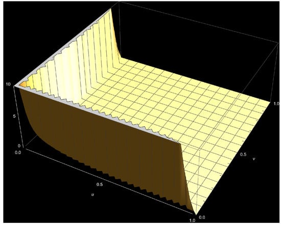
Figure A1.
The bivariate Kumaraswamy density (Equation (1)) plot, where and
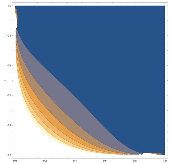
Figure A2.
The bivariate Kumaraswamy contour (Equation (1)) plot, where and
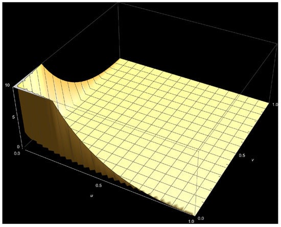
Figure A3.
The bivariate Kumaraswamy density (Equation (1)) plot, where and
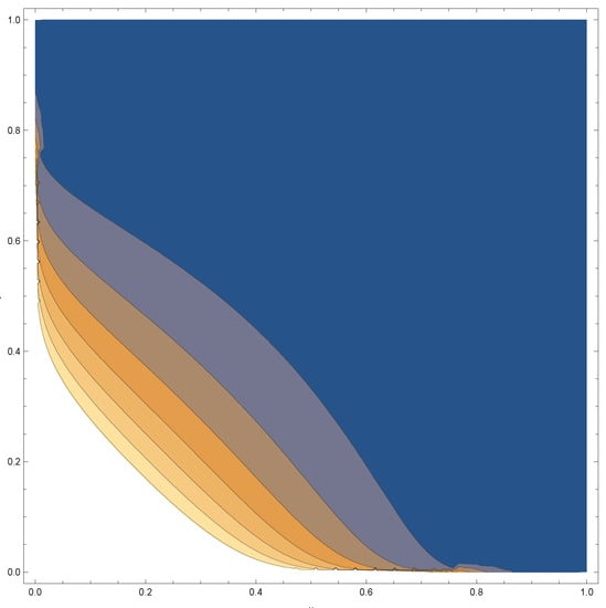
Figure A4.
The bivariate Kumaraswamy contour (Equation (1)) plot, where and
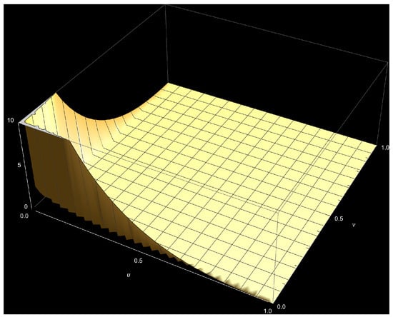
Figure A5.
The bivariate Kumaraswamy density (Equation (1)) plot, where and
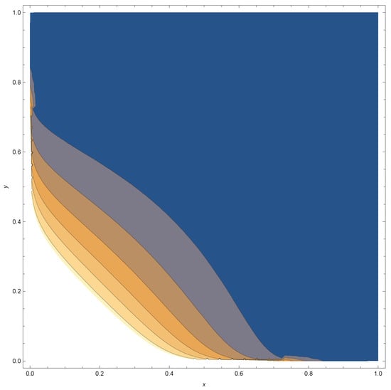
Figure A6.
The bivariate Kumaraswamy contour (Equation (1)) plot, where and
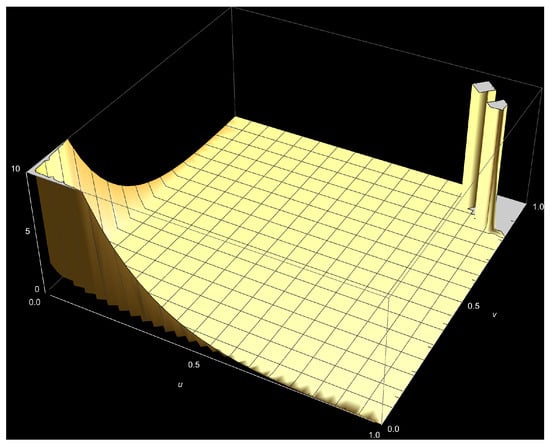
Figure A7.
The bivariate Kumaraswamy density (Equation (1)) plot, where and
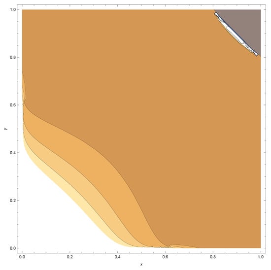
Figure A8.
The bivariate Kumaraswamy contour (Equation (1)) plot, where and
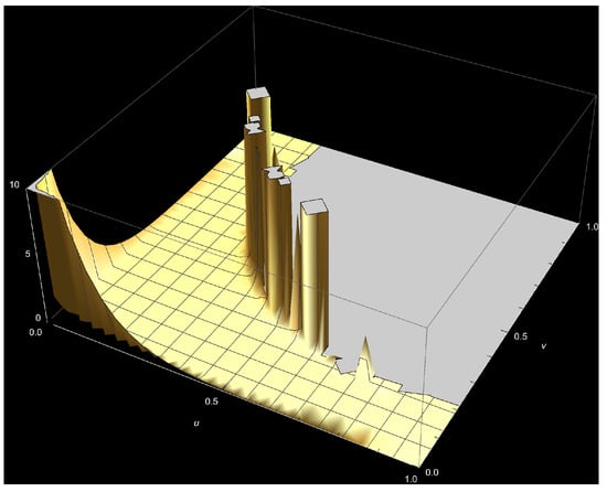
Figure A9.
The bivariate Kumaraswamy density (Equation (1)) plot, where and
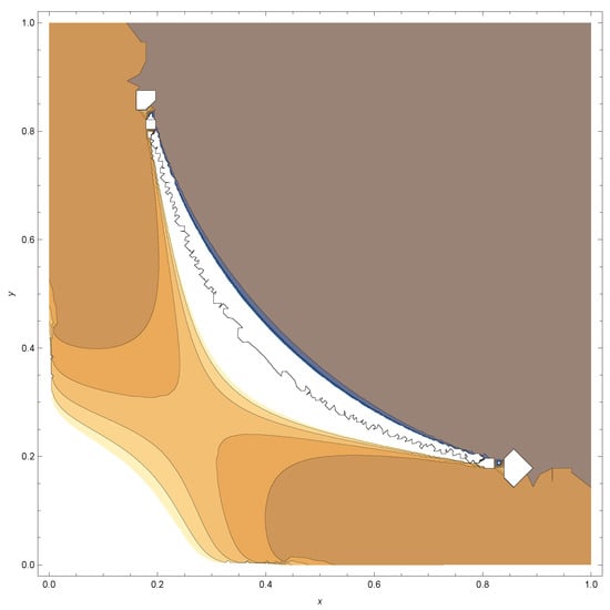
Figure A10.
The bivariate Kumaraswamy contour (Equation (1)) plot, where and
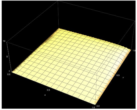
Figure A11.
The bivariate Kumaraswamy density (Equation (1)) plot, where and
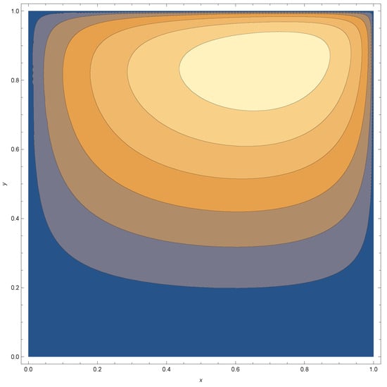
Figure A12.
The bivariate Kumaraswamy contour (Equation (1)) plot, where and
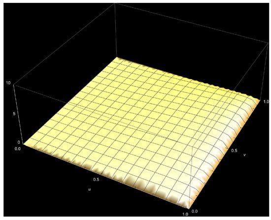
Figure A13.
The bivariate Kumaraswamy density (Equation (1)) plot, where and
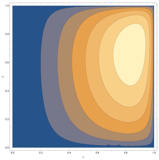
Figure A14.
The bivariate Kumaraswamy contour (Equation (1)) plot, where and
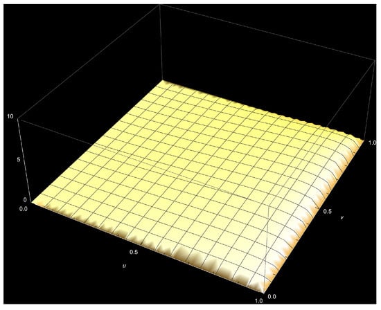
Figure A15.
The bivariate Kumaraswamy density (Equation (1)) plot, where and
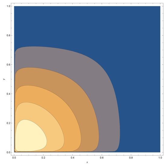
Figure A16.
The bivariate Kumaraswamy contour (Equation (1)) plot, where and
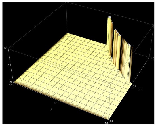
Figure A17.
The bivariate Kumaraswamy density (Equation (1)) plot, where and
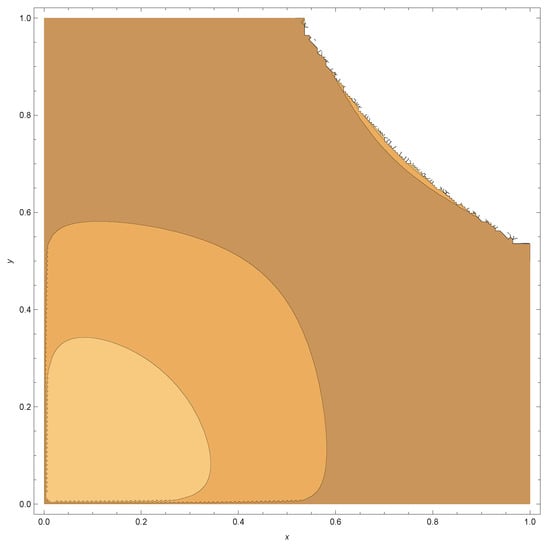
Figure A18.
The bivariate Kumaraswamy contour (Equation (1)) plot, where and
Scatterplots and marginal density plots are shown for the first data set based on the bivariate KW-type model in Equation (1).
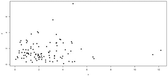
Figure A19.
The scatter plot for the first data set.
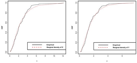
Figure A20.
The bivariate KW marginal densities (Equation (1)) plot for the first data set.
References
- Barreto-Souza, W.; Lemonte, A.J. Bivariate Kumaraswamy distribution: Properties and a new method to generate bivariate classes. Statistics 2013, 47, 1321–1342. [Google Scholar] [CrossRef]
- Ghosh, I. Bivariate and multivariate weighted Kumaraswamy distributions: Theory and applications. J. Stat. Theory Appl. 2019, 18, 198. [Google Scholar] [CrossRef]
- Arnold, B.C.; Ghosh, I. Some alternative bivariate Kumaraswamy models. Commun. Stat.-Theory Methods 2017, 46, 9335–9354. [Google Scholar] [CrossRef]
- Arnold, B.C.; Ng, H.K.T. Flexible bivariate beta distributions. J. Multivariate Anal. 2011, 102, 1194–1202. [Google Scholar] [CrossRef]
- Nadarajah, S.; Cordeiro, G.M.; Ortega, E.M. General results for the Kumaraswamy-G distribution. J. Stat. Comput. Simul. 2012, 82, 951–979. [Google Scholar] [CrossRef]
- Arnold, B.C.; Ghosh, I. Bivariate Kumaraswamy models involving use of Arnold-Ng copulas. J. Appl. Stat. Sci. 2017, 22, 227–241. [Google Scholar]
- Özel, G. Bivariate Kumaraswamy distribution with an application on earthquake data. AIP Conf. Proc. 2014, 1648, 610002. [Google Scholar]
- Chatfield, C. A marketing application of a characterization theorem. In A Modern Course on Distributions in Scientific Work; 2, Model Building and Model Selection; Patil, G.P., Kotz, S., Ord, J.K., Eds.; Reidel: Dordrecht, The Netherlands, 1975; pp. 175–185. [Google Scholar]
- Hoyer, R.W.; Mayer, L.S. The Equivalence of Various Objective Functions in a Stochastic Model of Electoral Competition; Technical Report No. 114, Series 2; Department of Statistics, Princeton University: Princeton, NJ, USA, 1976. [Google Scholar]
- Tong, Y.L. Probability Inequalities in Multivariate Distributions; Academic Press: New York, NY, USA, 1980. [Google Scholar]
- Nadarajah, S. The bivariate F3-beta distribution. Commun. Korean Math. Soc. 2006, 21, 363–374. [Google Scholar] [CrossRef]
- Nadarajah, S. A new bivariate beta distribution with application to drought data. Metron 2007, 65, 153–174. [Google Scholar]
Disclaimer/Publisher’s Note: The statements, opinions and data contained in all publications are solely those of the individual author(s) and contributor(s) and not of MDPI and/or the editor(s). MDPI and/or the editor(s) disclaim responsibility for any injury to people or property resulting from any ideas, methods, instructions or products referred to in the content. |
© 2023 by the author. Licensee MDPI, Basel, Switzerland. This article is an open access article distributed under the terms and conditions of the Creative Commons Attribution (CC BY) license (https://creativecommons.org/licenses/by/4.0/).