Robust Kibria Estimators for Mitigating Multicollinearity and Outliers in a Linear Regression Model

Abstract

In the presence of multicollinearity, the ordinary least squares (OLS) estimators, aside from BLUE (best linear unbiased estimator), lose efficiency and fail to achieve minimum variance. In addition, these estimators are highly sensitive to outliers in the response direction. To overcome these limitations, robust estimation techniques are often integrated with shrinkage methods. This study proposes a new class of Kibria Ridge M-estimators specifically developed to simultaneously address multicollinearity and outlier contamination. A comprehensive Monte Carlo simulation study is conducted to evaluate the performance of the proposed and existing estimators. Based on the mean squared error criterion, the proposed Kibria Ridge M-estimators consistently outperform the traditional ridge-type estimators under varying parameter settings. Furthermore, the practical applicability and superiority of the proposed estimators are validated using the Tobacco and Anthropometric datasets. Overall, the new proposed estimators demonstrate good performance, offering robust and efficient alternatives for regression modeling in the presence of multicollinearity and outliers.

1. Introduction

In regression analysis, the ordinary least squares (OLS) estimator is one of the most widely used techniques, relying on the assumptions that the explanatory variables are independent and that the error terms are homoscedastic and devoid of outliers. In the presence of multicollinearity and outliers in the predictor variables, OLS estimates become unstable, often exhibiting wrong signs and inflated variances that lead to incorrect inferences. Multicollinearity, a condition characterized by strong linear relationships among predictors, was first introduced by Ragnar Frisch in the 1930s [1]. It has since emerged as a fundamental area of interest in econometrics and regression modeling [2]. Severe multicollinearity reduces the clarity of regression coefficient interpretation, increases their standard errors, and lowers the overall precision and reliability of the model. Although ridge regression may enhance prediction accuracy through variance reduction, its dominance over OLS is not universal; it depends on the quantity of multicollinearity, the signal-to-noise ratio, and the error variance. As a result, it becomes difficult to discern the distinct contributions of each predictor, which could have a negative impact on model inference and prediction. Ridge Regression (RR) [3] provides a strong substitute to get around these restrictions by providing a controlled bias via a shrinkage parameter. This modification lowers variation, lessens the negative impacts of multicollinearity, and improves the general stability and accuracy of the coefficient estimations. More precisely, RR adds a bias term that is managed by the ridge tuning parameter $\left(k\right)$. The selection of k has a direct impact on the estimator’s mean squared error (MSE) and is essential in establishing the trade-off between bias and variance. Various methods for selecting the optimal k have been proposed in the literature, reflecting the continuous evolution of ridge-type estimators, see e.g.,  Hoerl and Kennard [3], Kibria [4], Khalaf et al. [5], and Dar and Chand. [6]. Outliers are observations that significantly depart from the typical data pattern. They can cause heteroscedasticity and skew model estimate. Gujarati and Porter [7] highlighted that such extreme observations may violate the constant variance assumption, thereby compromising the reliability of OLS estimates. The presence of outliers not only biases parameter estimates but also inflates residual variability, making traditional estimation techniques less effective.

To address the dual challenge of multicollinearity and outliers, Silvapulle [8] proposed the robust ridge or ridge M-estimator (RM), which combines the principles of RR and M-estimation. By incorporating robust loss functions and adaptive ridge parameters, the RM estimator enhances stability in the presence of both multicollinearity and data contamination. Recent studies have extended this framework, suggesting modified ridge M-estimators (MRM) that yield improved performance in terms of MSE and robustness, e.g.,  Ertas [9], Yasin et al. [10], Majid et al. [11], Wasim et al. [12], Alharthi [13,14], and Akhtar et al. [15].

To address the challenges posed by multicollinearity and outliers, this study introduces a class of Kibria-type ridge M-estimators designed to achieve robustness and stability under such adverse conditions. Following the structure of Kibria [4], we proposed five ridge-type estimators that simultaneously address high predictor intercorrelation and data contamination, thereby improving estimation efficiency and reliability. Using extensive simulations and two real-world datasets, the performance of the proposed estimators is compared with that of well-known existing estimators through the MSE criterion.

The remainder of this paper is structured as follows: Section 2 elaborates on the methodological framework, providing an overview of the existing ridge-type estimators and the formulation of the proposed estimators. Section 3 outlines the Monte Carlo simulation design used to evaluate the performance of the estimators. Section 4 presents a detailed analysis of the simulation findings along with their interpretation. Section 5 demonstrates the applicability and practical relevance of the proposed estimators through two real-data examples. Finally, Section 6 summarizes the key findings and concludes the study with possible directions for future research.

2. Methodology

Consider the standard multiple linear regression model:

$$Y=X\beta +ϵ$$

(1)

where $Y=(Y_1, Y_2, \dots , Y_n{)}^{\prime }$ is an $n\times 1$ vector of response variable and

$$X=\left[\begin{array}{cccc}{X}_{11}& X_{12}& \dots & X_{1p}\\ X_{21}& X_{22}& \dots & X_{2p}\\ ⋮& ⋮& \ddots & ⋮\\ X_{n1}& X_{n2}& \dots & X_{np}\end{array}\right]$$

is a $n\times p$ matrix (also known as design matrix) of the observed regressors, $\beta =({\beta }_1, {\beta }_2, \dots , {\beta }_p{)}^{\prime }$ is a $p\times 1$ vector of unknown regression parameters, and  $ϵ=({ϵ}_1, {ϵ}_2, \dots , {ϵ}_n{)}^{\prime }$ is an $n\times 1$ vector of random errors. $ϵ$ is independently and identically distributed with a zero mean and a covariance matrix ${\sigma }^2{I}_n$, where $I_n$ represents an identity matrix of order n. The OLS estimator can be estimated as

$${\widehat{\beta }}_{OLS}={\left(X^{T}X\right)}^{-1}{X}^{T}y$$

(2)

which depends primarily on the characteristics of the matrix ${\left(X^{T}X\right)}^{-1}$, that is, when the predictors are perfectly correlated, it is impossible to find the inverse of the matrix $\left(X^{T}X\right)$, so that the matrix becomes ill-conditioned [16,17].

To address this issue, Hoerl and Kennard [3] introduced the concept of the RR. In this method, a non-negative constant, known as the ridge parameter (k), is added to the diagonal elements of $\left(X^{T}X\right)$. This adjustment helps control the bias of the regression estimates towards the mean of the response variable, thereby stabilizing the estimator variability and mitigating the effects of multicollinearity. The RR estimator is defined as

$${\widehat{\beta }}_{RR}={(X^{T}X+kI)}^{-1}{X}^{T}y.$$

Then, the equation can be written as

$${\widehat{\beta }}_{RR}=R_k{\widehat{\beta }}_{OLS}$$

(3)

where $R_k={(X^{T}X+kI)}^{-1}{X}^{T}X$. The ${\widehat{\beta }}_{RR}$ estimator may exhibit bias; however, it generally has a lower MSE compared to the OLS estimator.

In the presence of multicollinearity and outliers, the MSE of both the OLS and RR estimators are inflated. To address this issue, Silvapulle [8] proposed a robust ridge M-estimator (RRM) by substituting ${\widehat{\beta }}_{OLS}$ with ${\widehat{\beta }}_M$ in Equation (3), as follows:

$${\widehat{\beta }}_{RRM}=R_k{\widehat{\beta }}_M$$

(4)

where ${\widehat{\beta }}_M$ is called M-estimator which can be obtained by solving the equation ${\sum }_{i=1}^n\mathrm{\Psi }\left({\displaystyle \frac{e_i}{s}}\right)=0$ and ${\sum }_{i=1}^n\mathrm{\Psi }\left({\displaystyle \frac{e_i}{s}}\right)x_i=0$, where $e_i$ are the residuals and obtained as $e_i=Y_i-x_i^T{\widehat{\beta }}_M$ and $\mathrm{\Psi }$ is a function used to adjust how much weight each residual contributes to the overall fitting process. This function also depend on whether the estimator has good large sample theory [18]. The above equations together describe the conditions under which the robust estimator achieves a balance between the residuals and the predictor variables, with $\mathrm{\Psi }$ function ensuring that outliers have a limited effect on this balance. According to Montgomery et al. [19], s is a robust estimate of scale. A popular choice for s is the median absolute deviation defined as:

$$s={\displaystyle \frac{\mathrm{median}\left(|e_i-\mathrm{median}\left(e_i\right)|\right)}{0.6745}}$$

The tuning constant 0.6745 makes s an approximately unbiased estimator of $\sigma$ if n is large and the error distribution is normal. The choice of $\mathrm{\Psi }$ function depends on the desired level of robustness and the type of deviations from the classical assumptions (e.g., outliers, heavy tails) [20].

2.1. Canonical Form

Suppose that Q is a ($p\times p$) orthogonal matrix such that $Q^{T}Q=I_n$ and $Q^T{X}^{T}XQ=\mathrm{\Lambda }$, where $\mathrm{\Lambda }=\mathrm{diag}({\lambda }_1, {\lambda }_2, \dots , {\lambda }_p)$ contains the eigenvalues of the matrix $\left(X^{T}X\right)$. Then, the canonical form of model (1) is expressed as:

$$y=Z\alpha +ϵ.$$

Given that $Z=XQ$, the vector of estimates $\widehat{\alpha }={({\alpha }_1, {\alpha }_2, \dots , {\alpha }_p)}^T$ can be expressed as $Q^T\widehat{\beta }$, where $\widehat{\beta }=Q\widehat{\alpha }$. Moreover, the MSE of $\widehat{\alpha }$ is equal to the MSE of $\widehat{\beta }$. The canonical form for Equations (2)–(4) can be written as:

$${\widehat{\alpha }}_{OLS}={\mathrm{\Lambda }}^{-1}{Z}^{T}y$$

$${\widehat{\alpha }}_{RR}={(\mathrm{\Lambda }+kI)}^{-1}\mathrm{\Lambda }{\widehat{\alpha }}_{OLS}$$

$${\widehat{\alpha }}_{RRM}={(\mathrm{\Lambda }+kI)}^{-1}\mathrm{\Lambda }{\widehat{\alpha }}_M$$

where $k=\mathrm{diag}(k_1, k_2, \dots , k_p)$, $(k_j>0)$ for j=1,2, …, p. Following [21], the MSE of above estimators are given as follows:

$$\mathrm{MSE}\left({\widehat{\alpha }}_{OLS}\right)={\widehat{\sigma }}^2\sum _{i=1}^p{\displaystyle \frac{1}{{\lambda }_i}}$$

$$\mathrm{MSE}\left({\widehat{\alpha }}_M\right)=\sum _{i=1}^p{\mathrm{\Omega }}_{ii}$$

$$\mathrm{MSE}\left({\widehat{\alpha }}_{RR}\right)={\widehat{\sigma }}^2\sum _{j=1}^p{\displaystyle \frac{{\lambda }_j}{{({\lambda }_j+k_j)}^2}}+\sum _{j=1}^p{\displaystyle \frac{k_j^2{\widehat{\alpha }}_{j\left(OLS\right)}^2}{{({\lambda }_j+k_j)}^2}}$$

(5)

$$\mathrm{MSE}\left({\widehat{\alpha }}_{RRM}\right)=\sum _{j=1}^p{\displaystyle \frac{{\mathrm{\Omega }}_{ii}{\lambda }_j^2}{{({\lambda }_j+k_j)}^2}}+\sum _{j=1}^p{\displaystyle \frac{k^2{\widehat{\alpha }}_{Mj}^2}{{({\lambda }_j+k)}^2}}$$

(6)

where ${\widehat{\sigma }}^2$ represents the least square estimator of error variance of the model 1, ${\widehat{\alpha }}_{Mj}$ is the $j^{th}$ value of $\widehat{\alpha }$ and ${\lambda }_j$ is the $j^{th}$ eigenvalue of the matrix $X^{T}X$, ${\mathrm{\Omega }}_{ii}$ are the diagonal elements of the matrix $\mathrm{\Omega }=\mathrm{Cov}\left({\widehat{\alpha }}_M\right)$. Furthermore, ref. [21] showed that

$$\mathrm{MSE}\left({\widehat{\alpha }}_{\mathrm{RRM}}\right)<\mathrm{MSE}\left({\widehat{\alpha }}_{\mathrm{M}}\right) \mathrm{and} \mathrm{MSE}\left({\widehat{\alpha }}_{\mathrm{RRM}}\right)<\mathrm{MSE}\left({\widehat{\alpha }}_{\mathrm{RR}}\right)$$

if ${\mathrm{\Omega }}_{ii}<{\sigma }^2{\lambda }_i^{-1}$, where $i=1, 2,\dots , p.$

2.2. Existing Estimators

This section describes some of the popular and widely used ridge estimators defined in Equations (7)–(13). The pioneer work of [3] introduced the estimator of $k_j$ as the ratio of estimated error variance ${\widehat{\sigma }}^2$ and $j^{th}$ estimate of $\alpha$ using OLS as

$$\widehat{k_j}={\displaystyle \frac{{\widehat{\sigma }}^2}{{\widehat{\alpha }}_j^2}}, j=1, 2, \dots , p$$

where ${\widehat{\sigma }}^2={\displaystyle \frac{\sum e_i^2}{n-p}}$.

Later, ref. [3] suggested the following estimator to determine a single value for k,

$${\widehat{k}}_{HK}={\displaystyle \frac{{\widehat{\sigma }}^2}{{\widehat{\alpha }}_{max}^2}}$$

(7)

where ${\widehat{\alpha }}_{\max }=max({\alpha }_1, {\alpha }_2, \dots , {\alpha }_p)$.

In another study, ref. [22] proposed the ridge parameter by using harmonic mean of $\widehat{k_j}$ as

$${\widehat{k}}_{HKB}={\displaystyle \frac{p{\widehat{\sigma }}^2}{\sum {\widehat{\alpha }}_j^2}}$$

(8)

Furthermore, ref. [4] introduced five additional ridge estimators, which are defined as follows:

$$k_{KIB1}=GM\left({\displaystyle \frac{{\widehat{\sigma }}^2}{{\widehat{\alpha }}_i^2}}+{\displaystyle \frac{1}{{\lambda }_i}}\right),$$

(9)

where GM stands for geometric mean.

$$k_{KIB2}=HM\left({\displaystyle \frac{{\widehat{\sigma }}^2}{{\widehat{\alpha }}_i^2}}+{\displaystyle \frac{1}{{\lambda }_i}}\right),$$

(10)

where HM stands for harmonic mean.

$$k_{KIB3}=Median\left({\displaystyle \frac{{\widehat{\sigma }}^2}{{\widehat{\alpha }}_i^2}}+{\displaystyle \frac{1}{{\lambda }_i}}\right)$$

(11)

$$k_{KIB4}=max\left({\displaystyle \frac{{\widehat{\sigma }}^2}{{\widehat{\alpha }}_i^2}}+{\displaystyle \frac{1}{{\lambda }_i}}\right),$$

(12)

where max stands for maximum.

$$k_{KIB5}=min\left({\displaystyle \frac{{\widehat{\sigma }}^2}{{\widehat{\alpha }}_i^2}}+{\displaystyle \frac{1}{{\lambda }_i}}\right),$$

(13)

where min stands for minimum.

2.3. Proposed Estimators

Previous studies by McDonald and Galarneau [23], McDonald [24], and Majid et al. [25] demonstrated that the optimal choice of the biasing parameter for the RM is primarily influenced by several factors, including the degree of multicollinearity, presence of outliers, number of predictors, error variance, the underlying error distribution, and sample size. According to Suhail et al. [26], when datasets exhibit severe multicollinearity combined with a large number of predictors, substantial error variance, and large sample sizes, the conventional RM estimators often fail to achieve the minimum MSE. To address these limitations, it becomes essential to develop improved RM estimators that maintain efficiency under adverse conditions, such as high multicollinearity, large error variance, increased sample size, and the presence of influential outliers in the response direction.

Following the suggestion of Silvapulle [8], the robust version can be obtained by replacing ${\widehat{\sigma }}^2$ with ${\widehat{A}}^2$ and ${\widehat{\alpha }}^2$ with ${\widehat{\alpha }}_M^2$. Using Huber function [20], ${\widehat{A}}^2$ can be obtained as

$${\widehat{A}}^2={\displaystyle \frac{{\displaystyle n^2{s}^2\sum _{i=1}^n{\mathrm{\Psi }}^2(e_i/s)}}{(n-p){\left({\displaystyle \sum _{i=1}^n{\mathrm{\Psi }}^{\prime }(e_i/s)}\right)}^2}}.$$

where $\mathrm{\Psi }\left(·\right)$ denotes the Huber weight function, n is the sample size, and p is the number of predictors. Building upon this idea, we propose the following robust versions of the ridge estimators originally introduced by Kibria [4].

$$k_{KIB.M.1}=GM\left({\displaystyle \frac{A^2}{{\alpha }_{M_j}^2}}+{\displaystyle \frac{1}{{\lambda }_i}}\right),$$

(14)

$$k_{KIB.M.2}=HM\left({\displaystyle \frac{A^2}{{\alpha }_{M_j}^2}}+{\displaystyle \frac{1}{{\lambda }_i}}\right),$$

(15)

$$k_{KIB.M.3}=Median\left({\displaystyle \frac{A^2}{{\alpha }_{M_j}^2}}+{\displaystyle \frac{1}{{\lambda }_i}}\right),$$

(16)

$$k_{KIB.M.4}=max\left({\displaystyle \frac{A^2}{{\alpha }_{M_j}^2}}+{\displaystyle \frac{1}{{\lambda }_i}}\right),$$

(17)

$$k_{KIB.M.5}=min\left({\displaystyle \frac{A^2}{{\alpha }_{M_j}^2}}+{\displaystyle \frac{1}{{\lambda }_i}}\right),$$

(18)

where $GM$, $HM$, max, and min are defined as mentioned above. Each of these proposed estimators incorporates a robust measure of dispersion ($A^2$) and modified eigenvalue structure (${\alpha }_{M_j}$), thereby enhancing stability and reliability in the presence of multicollinearity and influential observations.

3. Simulation Setup

A simulation-based investigation was carried out in which the datasets were deliberately constructed to reflect predefined levels of multicollinearity. Using these datasets, the performance of the ridge estimators and the proposed ridge M-estimators was evaluated. The simulation study generated data sets that varied across several factors: the number of regressors ($p=4, 10$), the sample size ($n=25, 50, 100$), the degree of multicollinearity among predictors ($\rho =0.85, 0.95, 0.99, 0.999$), and the presence of outliers in the response variable. Additionally, different levels of error variance were considered by setting ${\sigma }^2=0.1, 1, 2, 5$, enabling a thorough evaluation of estimator performance in a range of data scenarios. Following ref. [23] and the more recent implementations in ref. [27], the predictor variables were generated as

$$x_{ij}=\sqrt{1-{\rho }^2} v_{ij}+\rho v_{i(p+1)}, i=1, \dots , n, j=1, \dots , p,$$

(19)

where $v_{ij}$ are independent draws from the standardized normal distribution, and $\rho$ controls the pairwise correlation between predictor variables. To study different levels of multicollinearity. The dependent variable was generated by the usual linear model

$$y_i={\beta }_0+\sum _{j=1}^p{\beta }_j{x}_{ji}+{\epsilon }_i, i=1, \dots , n,$$

(20)

where ${\epsilon }_i\stackrel{\mathrm{iid}}{\sim }N(0, {\sigma }^2)$. In line with ref. [26], and ref. [27], we set ${\beta }_0=0$ and chose the coefficient vector $\beta ={({\beta }_1, \dots , {\beta }_p)}^T$ to be the normalized eigenvector corresponding to the largest eigenvalue of the $X^{T}X$ matrix so that ${\beta }^T\beta =1$.

• To examine robustness, we contaminated the response by introducing outliers by considering 10% and 20% contamination levels. For each contamination level, a corresponding fraction of observations was replaced by outliers whose errors were drawn from a distribution with inflated variance. Concretely, if the nominal error variance is ${\sigma }^2$, the contaminated error variance was taken as

$${\sigma }^{2\ast }=\left\{\begin{array}{cc}{\sigma }^2+10,\hfill & \mathrm{for} 10\% \mathrm{outliers},\hfill \\ {\sigma }^2+20,\hfill & \mathrm{for} 20\% \mathrm{outliers}.\hfill \end{array}\right.$$

Additionally, to evaluate the performance of the proposed estimators under heavy-tailed error structures, the error term is modeled using the standardized Cauchy distribution, i.e., ${\epsilon }_i\sim \mathrm{Cauchy}(0, 1)$, having mean 0 and scale parameter 1. This distribution is known for its heavy tails and the absence of finite variance, providing a challenging environment to assess the robustness of the estimators. For each configuration we performed 5000 Monte Carlo replications. All computations were implemented in the R programming language. In contrast with robust estimation, the objective function (Huber loss) [20] was used to compute M-estimators via the rlm() function (from the MASS package). In a code-style notation, it can be written as

$$\mathtt{rlm}(\mathtt{formula}, \mathtt{weights}, \mathtt{acc}=\mathtt{0}.\mathtt{01})$$

where formula is the fitted model (e.g., $y\sim x_1+x_2+\dots$), weights is an optional prior-weights vector, and acc sets the convergence tolerance for the iterative algorithm. The Huber loss is widely used in robust regression because it combines quadratic behavior near zero (efficiency) with linear tails (robustness) [19].

The MSE criterion has been used to compare the performance of estimators. Mathematically, it is given as

$$MSE\left({\widehat{\alpha }}_i\right)={\displaystyle \frac{1}{W}}\sum _{i=1}^W\sum _{j=1}^p{({\widehat{\alpha }}_{ij}-{\alpha }_j)}^2, i=1, 2, 3, \dots , W$$

where $W=5000$ indicates the number of Monte Carlo runs. The objective is to achieve an MSE value close to zero. The MSEs of the ridge estimator are influenced by the shrinkage parameter k, which in turn depends on factors such as the sample size n, the number of predictors p, the variance ${\sigma }^2$, and the correlation $\rho$.

4. Results and Discussion

Table 1 lists the MSE values of the OLS, ridge-type (RR, HKB, KIB1–KIB5), M-estimator, and proposed Kibria M-type estimators (KIB.M.1–KIB.M.5) under various levels of multicollinearity ($\rho =0.85, 0.95, 0.99, 0.999$) and error variances (${\sigma }^2=0.1, 1, 2, 5$) for $n=25$, $p=4$, and a 10% outlier contamination in the response direction. The results indicate that the OLS and conventional ridge estimators (RR, HKB) exhibit substantially higher MSE values under strong multicollinearity and higher variance conditions. In contrast, the proposed KIB.M estimators, particularly KIB.M.1 and KIB.M.2 consistently yield smaller MSE values across most settings, demonstrating greater robustness to outliers and efficiency compared to existing estimators. These findings highlight the improved performance of the proposed estimators, especially when both multicollinearity and outliers are present in the data.

Table 1. Estimated MSE with $n=25$, $p=4$, and 10% outlier in response direction.

	${\mathit{\sigma }}^2=0.1$				${\mathit{\sigma }}^2=1$
$\mathit{\rho }$	0.85	0.95	0.99	0.999	0.85	0.95	0.99	0.999
OLS	58.0927	185.8187	936.4001	9456.9941	64.7814	200.9017	1027.8460	9934.8098
RR	29.2387	92.7448	462.6969	4659.9051	32.6498	100.2520	513.8670	4890.4584
HKB	16.0564	48.2692	233.0434	2335.5599	17.8622	52.1160	261.2628	2438.7259
KIB1	4.0498	3.1330	0.7468	0.4406	4.3422	3.4322	0.9521	0.4542
KIB2	13.0830	17.1324	2.8068	0.4546	14.5109	18.4365	3.2207	0.4792
KIB3	2.4550	1.6340	0.6878	0.4614	2.9896	2.2370	0.9313	0.4715
KIB4	24.0229	41.2881	16.2383	0.5389	26.8355	44.3018	17.9198	0.5713
KIB5	0.6839	0.5634	0.5027	0.4427	0.7678	0.6318	0.5393	0.4485
M	0.0126	0.0439	0.1934	1.9562	1.2290	3.8524	18.9445	187.6748
KIB.M.1	0.0146	0.0128	0.0074	0.0039	0.3050	0.4178	0.1420	0.0356
KIB.M.2	0.0117	0.0315	0.0862	0.0935	0.4483	0.5975	0.2361	0.0294
KIB.M.3	0.0474	0.0210	0.0064	0.0396	0.3682	0.5194	0.1570	0.0518
KIB.M.4	0.0123	0.0367	0.1480	0.4358	0.6649	0.9991	0.6996	0.1491
KIB.M.5	0.3398	0.2055	0.1019	0.2300	0.4188	0.3584	0.1350	0.2386
	${\mathit{\sigma }}^{\mathbf{2}}=\mathbf{2}$				${\mathit{\sigma }}^{\mathbf{2}}=\mathbf{5}$
$\mathit{\rho }$	0.85	0.95	0.99	0.999	0.85	0.95	0.99	0.999
OLS	70.1926	208.0636	1089.2582	10,876.7420	99.2650	310.1080	1559.9584	15,585.7510
RR	35.3699	103.8109	540.8278	5416.4407	51.4518	158.8139	796.0424	7934.8257
HKB	19.2568	53.9170	274.5583	2720.5292	27.7163	82.4260	404.7256	3995.6074
KIB1	4.4677	3.8790	1.2324	0.4716	6.3324	6.6642	2.1039	0.6972
KIB2	15.5338	19.1306	3.7175	0.5067	21.6009	27.8779	6.0095	0.7444
KIB3	3.5403	3.3627	1.3714	0.4906	6.7121	9.8640	2.9349	0.7139
KIB4	29.1181	45.4389	18.9927	0.6110	42.1642	64.2844	25.9303	0.9062
KIB5	0.8249	0.6931	0.5781	0.4381	1.0747	0.9391	0.7777	0.5340
M	4.8400	15.1401	73.6704	753.1448	29.9525	89.5449	448.3138	4502.3748
KIB.M.1	0.8556	1.1041	0.3248	0.0801	3.0708	3.7903	1.0271	0.2912
KIB.M.2	1.3293	1.6746	0.4455	0.0752	7.0004	8.7127	1.9626	0.2990
KIB.M.3	0.9593	1.2175	0.3535	0.0775	3.2315	5.3138	1.1511	0.2949
KIB.M.4	2.2610	3.2010	1.1464	0.1108	13.7509	18.6388	6.4040	0.3327
KIB.M.5	0.6019	0.5629	0.2098	0.2455	0.9615	0.8365	0.5076	0.3446

Note: Bold values show the minimum MSE of estimators (per column).

Table 2 displays the MSE values of the OLS, ridge-type, M-, and proposed KIB.M estimators for the case of $n=50$, $p=4$, and 10% outliers in the response (second scenario). The results are reported under varying degrees of multicollinearity ($\rho =0.85, 0.95, 0.99, 0.999$) and different error variances (${\sigma }^2=0.1, 1, 2, 5$). As expected, the MSE values of the conventional estimators (OLS, RR, and HKB) increase sharply with higher $\rho$ and ${\sigma }^2$, indicating their sensitivity to multicollinearity and outlier contamination. In contrast, the proposed KIB.M estimators, particularly KIB.M.1, KIB.M.2, and KIB.M.3, maintain smaller and more stable MSE values across all conditions indicating their improved efficiency and robustness properties when compared with traditional and ridge-type estimators. The results further confirm that the proposed estimators perform consistently well even when sample size increases, demonstrating their reliability and adaptability under different error structures for large sample.

Table 2. Estimated MSE with $n=50$, $p=4$, and 10% outlier in response direction.

	${\mathit{\sigma }}^2=0.1$				${\mathit{\sigma }}^2=1$
$\mathit{\rho }$	0.85	0.95	0.99	0.999	0.85	0.95	0.99	0.999
OLS	34.6946	117.2798	650.7218	6792.6861	36.5320	125.4283	702.5415	7316.4849
RR	15.6560	52.6148	288.8304	3086.8632	16.3158	56.4934	317.6253	3307.2420
HKB	8.7046	26.4883	141.0854	1492.0072	8.9762	28.6283	155.0535	1597.0226
KIB1	3.7903	5.4993	2.0934	0.6609	3.8194	5.8765	2.1430	0.6990
KIB2	8.3114	16.4146	5.3940	0.6934	8.5615	17.8317	5.7228	0.7314
KIB3	4.8377	9.6448	3.4662	0.6819	4.7905	10.3593	3.6203	0.7203
KIB4	14.9987	34.9131	17.5369	0.7764	15.6363	38.0806	18.9561	0.8196
KIB5	1.1306	0.9854	0.7593	0.5296	1.1243	0.9991	0.7667	0.5577
M	0.0080	0.0265	0.1421	1.4494	0.7665	2.6527	14.0815	146.8372
KIB.M.1	0.0085	0.0094	0.0079	0.0010	0.1965	0.3401	0.1549	0.0173
KIB.M.2	0.0077	0.0233	0.0797	0.1216	0.3135	0.5169	0.2331	0.0212
KIB.M.3	0.0371	0.0151	0.0049	0.0093	0.2330	0.4402	0.1957	0.0190
KIB.M.4	0.0079	0.0256	0.1189	0.4721	0.4645	0.8311	0.5694	0.1151
KIB.M.5	0.3020	0.1797	0.0839	0.0893	0.3457	0.2983	0.1218	0.0977
	${\mathit{\sigma }}^{\mathbf{2}}=\mathbf{2}$				${\mathit{\sigma }}^{\mathbf{2}}=\mathbf{5}$
$\mathit{\rho }$	0.85	0.95	0.99	0.999	0.85	0.95	0.99	0.999
OLS	36.5320	125.4283	702.5415	7316.4849	59.3460	200.1127	1114.8463	11,353.1630
RR	16.3158	56.4934	317.6253	3307.2420	27.7894	93.0853	521.3718	5307.7716
HKB	8.9762	28.6283	155.0535	1597.0226	14.9574	46.6490	256.9009	2593.8125
KIB1	3.8194	5.8765	2.1430	0.6990	5.4922	7.4629	2.9712	0.9368
KIB2	8.5615	17.8317	5.7228	0.7314	13.9308	26.6379	8.7061	0.9901
KIB3	4.7905	10.3593	3.6203	0.7203	6.8415	13.2102	5.1824	0.9621
KIB4	15.6363	38.0806	18.9561	0.8196	26.2476	58.5495	28.9429	1.1219
KIB5	1.1243	0.9991	0.7667	0.5577	1.3480	1.1370	0.9915	0.7206
M	0.7665	2.6527	14.0815	146.8372	18.2339	61.6977	342.1877	3469.2562
KIB.M.1	0.1965	0.3401	0.1549	0.0173	2.0330	3.0332	1.0888	0.2226
KIB.M.2	0.3135	0.5169	0.2331	0.0212	4.5913	7.5814	2.4499	0.2239
KIB.M.3	0.2330	0.4402	0.1957	0.0190	2.0717	3.8740	1.3708	0.2313
KIB.M.4	0.4645	0.8311	0.5694	0.1151	8.7541	16.3392	7.8821	0.2447
KIB.M.5	0.3457	0.2983	0.1218	0.0977	0.7398	0.6048	0.3941	0.2423

Note: Bold values indicate the minimum MSE in each column.

Table 3 tabulates the MSE values of different estimators when considering $n=100$, $p=4$, and 10% outliers in the response (third scenario) with varying levels of multicollinearity ($\rho =0.85, 0.95, 0.99, 0.999$) and different error variances (${\sigma }^2=0.1, 1, 2, 5$). It is evident that the MSE values of OLS, RR, and HKB estimators increase rapidly with higher correlation and larger error variance, reflecting their sensitivity to multicollinearity and the presence of outliers. Conversely, the proposed KIB.M estimators, particularly KIB.M.1, KIB.M.2, and KIB.M.3, continue to demonstrate superior performance with substantially lower MSE values across all settings. This indicates that the proposed estimators are not only robust to outliers but also maintain their efficiency as the sample size increases. Overall, the results confirm that the KIB.M family performs consistently better than traditional and ridge-type estimators in large-sample scenario affected by multicollinearity and outlier contamination.

Table 3. Estimated MSE with $n=100$, $p=4$, and 10% outlier in response direction.

	${\mathit{\sigma }}^2=0.1$				${\mathit{\sigma }}^2=1$
$\mathit{\rho }$	0.85	0.95	0.99	0.999	0.85	0.95	0.99	0.999
OLS	19.0279	57.2612	274.5560	2828.1813	20.3774	60.8559	295.9322	2909.4998
RR	9.2954	27.4686	129.6406	1370.5442	9.9276	29.2102	141.1418	1370.9880
HKB	4.8297	13.5761	62.8932	669.3609	5.1218	14.5280	69.3756	662.3241
KIB1	2.0242	3.8027	4.4247	0.2550	2.0692	3.9624	4.7756	0.2705
KIB2	4.7483	11.6719	17.4909	0.4015	5.0287	12.5333	19.0874	0.4200
KIB3	2.0330	4.4982	9.1134	0.2846	2.1187	4.6830	10.1460	0.3036
KIB4	9.1803	24.4692	46.4281	1.0370	9.7998	26.0663	50.3187	1.0578
KIB5	0.6670	0.5109	0.3187	0.2353	0.6719	0.5277	0.3409	0.2503
M	0.0034	0.0106	0.0517	0.5193	0.3504	1.0342	5.1510	50.8688
KIB.M.1	0.0058	0.0055	0.0110	0.0011	0.1135	0.2082	0.3324	0.0158
KIB.M.2	0.0034	0.0101	0.0420	0.1447	0.1942	0.3600	0.4802	0.0364
KIB.M.3	0.0403	0.0170	0.0073	0.0013	0.1336	0.2600	0.4211	0.0139
KIB.M.4	0.0034	0.0105	0.0489	0.3258	0.2694	0.5554	0.8636	0.2237
KIB.M.5	0.3272	0.1903	0.1003	0.0369	0.3381	0.2489	0.2108	0.0378
	${\mathit{\sigma }}^{\mathbf{2}}=\mathbf{2}$				${\mathit{\sigma }}^{\mathbf{2}}=\mathbf{5}$
$\mathit{\rho }$	0.85	0.95	0.99	0.999	0.85	0.95	0.99	0.999
OLS	21.9499	66.4085	326.5090	3234.1058	30.7153	92.6793	462.7390	4583.4807
RR	10.6937	32.0674	156.9901	1546.2310	15.3171	45.6449	226.8457	2238.7843
HKB	5.5440	15.9454	77.3465	762.3114	8.0016	22.9289	113.0043	1117.6602
KIB1	2.2371	4.2241	4.9129	0.2871	2.8970	5.3758	6.2166	0.3939
KIB2	5.4454	13.5978	20.8440	0.4565	7.8391	19.2260	28.5369	0.6476
KIB3	2.2604	5.0579	10.7974	0.3270	3.1496	7.3172	15.2774	0.4720
KIB4	10.5574	28.4571	55.6101	1.1692	15.1097	40.1772	75.5523	1.6447
KIB5	0.6939	0.5339	0.3458	0.2600	0.7575	0.5853	0.4216	0.3463
M	1.3356	4.1181	20.3138	203.1294	8.1954	24.7062	124.8416	1206.5115
KIB.M.1	0.3082	0.6035	0.8319	0.0384	1.1756	2.2572	2.6686	0.1397
KIB.M.2	0.4989	1.0338	1.3069	0.0466	2.3613	5.3627	6.9860	0.1770
KIB.M.3	0.3686	0.6936	0.8654	0.0502	1.1458	2.1805	3.9301	0.1345
KIB.M.4	0.7645	1.8536	2.9491	0.0896	4.2579	10.9848	18.0187	0.3888
KIB.M.5	0.3978	0.3893	0.3243	0.0461	0.5933	0.5159	0.2809	0.1320

Note: Bold values indicate the minimum MSE in each column.

Table 4, Table 5 and Table 6 present the estimated MSEs of the OLS, ridge-type, M, and proposed KIB.M estimators under varying conditions of sample size ($n=25, 50, 100$), number of explanatory variables ($p=10$) with the presence of 10% outliers in the response direction. Each scenario was analyzed for different degrees of multicollinearity ($\rho =0.85, 0.95, 0.99, 0.999$) and error variances (${\sigma }^2=0.1, 1, 2, 5$).

Table 4. Estimated MSE with $n=25$, $p=10$, and 10% outlier in response direction.

	${\mathit{\sigma }}^2=0.1$				${\mathit{\sigma }}^2=1$
$\mathit{\rho }$	0.85	0.95	0.99	0.999	0.85	0.95	0.99	0.999
OLS	694.9215	2187.0384	11,383.8803	112,600.5552	750.0080	2279.6316	12,127.9258	119,784.4872
RR	529.8690	1645.0894	8526.8235	84,002.6995	569.0494	1709.8681	9067.4344	89,557.5483
HKB	214.6990	664.8578	3464.0875	34,304.8833	229.8675	688.8306	3679.6501	36,678.8538
KIB1	12.7587	12.0948	1.9610	0.2352	13.4927	12.7382	2.0908	0.2510
KIB2	39.4742	37.8451	4.8604	0.2482	42.3634	40.0139	5.1855	0.2635
KIB3	22.1650	26.8116	3.3750	0.2480	23.8538	28.3230	3.5543	0.2631
KIB4	134.9462	126.0470	23.0533	0.3377	144.5934	133.7625	24.5508	0.3405
KIB5	0.6767	0.5761	0.3775	0.4148	0.7315	0.6166	0.3968	0.4322
M	0.1908	0.5957	3.0754	31.3217	18.0344	56.0237	290.4824	2916.6463
KIB.M.1	0.0156	0.0170	0.0035	0.0088	0.8855	0.9244	0.1408	0.0258
KIB.M.2	0.1162	0.2006	0.2707	0.1317	1.9445	1.8281	0.3478	0.0198
KIB.M.3	0.0169	0.0157	0.0026	0.0188	1.4388	1.4524	0.1867	0.0257
KIB.M.4	0.1782	0.4865	1.4732	2.6664	4.5866	5.0858	2.7318	0.5964
KIB.M.5	0.4109	0.2702	0.1411	0.3752	0.4770	0.3347	0.1467	0.3782
	${\mathit{\sigma }}^{\mathbf{2}}=\mathbf{2}$				${\mathit{\sigma }}^{\mathbf{2}}=\mathbf{5}$
$\mathit{\rho }$	0.85	0.95	0.99	0.999	0.85	0.95	0.99	0.999
OLS	810.9070	2517.8413	13,314.2722	134,567.7471	1047.9543	3309.4832	16,968.7928	168,822.5134
RR	610.6199	1880.1172	9911.1430	99,759.2796	767.3045	2400.1524	12,310.2106	122,303.6539
HKB	245.2323	760.7674	4030.5122	40,850.9594	305.5136	960.4464	4967.2802	49,527.6053
KIB1	15.0209	14.2878	2.2884	0.2819	20.0969	20.2169	3.0647	0.3692
KIB2	46.9245	44.8969	5.7439	0.2995	66.0779	63.9960	8.0038	0.3974
KIB3	26.5631	31.8188	3.8261	0.2968	37.9880	44.8311	5.1952	0.3898
KIB4	157.2672	150.2331	27.3002	0.3844	208.8650	214.0298	38.5394	0.5086
KIB5	0.8664	0.6758	0.4181	0.4352	1.0677	0.8236	0.5179	0.4527
M	65.5798	209.0153	1079.9024	10,852.4634	333.1045	1076.2807	5474.9648	57,562.0311
KIB.M.1	2.8035	3.0700	0.4137	0.0479	12.5061	13.2073	1.7051	0.1589
KIB.M.2	6.1524	5.9059	0.7721	0.0430	31.5744	31.2095	3.6162	0.1650
KIB.M.3	4.2106	4.3683	0.5555	0.0431	19.4487	21.9938	2.2811	0.1613
KIB.M.4	15.9285	17.4715	3.4439	0.2538	82.8792	96.4197	17.1214	0.2507
KIB.M.5	0.6213	0.5141	0.1600	0.3816	1.0072	0.9009	0.3059	0.4029

Note: Bold values indicate the minimum MSE in each column.

Table 5. Estimated MSE with $n=50$, $p=10$, and 10% outlier in the response direction.

	${\mathit{\sigma }}^2=0.1$				${\mathit{\sigma }}^2=1$
$\mathit{\rho }$	0.85	0.95	0.99	0.999	0.85	0.95	0.99	0.999
OLS	130.9014	387.9817	2000.6351	19,738.7721	141.2115	416.8765	2150.3620	21,294.1110
RR	74.9723	216.6013	1107.9338	10,938.4027	80.8513	230.6455	1193.5570	11,665.5611
HKB	34.4355	99.0109	504.6374	4962.3562	37.0364	104.8461	542.2782	5240.2312
KIB1	11.2235	18.8991	13.0523	0.3716	11.8465	19.2350	13.7957	0.4060
KIB2	30.5554	56.7551	40.6522	0.5356	32.7172	59.6432	43.3727	0.5878
KIB3	16.4514	33.5338	30.9676	0.4388	17.7104	34.7571	32.7685	0.4825
KIB4	67.7993	138.6428	160.6322	1.7594	72.6526	147.0998	171.2623	1.9245
KIB5	0.8676	0.7170	0.5179	0.2651	0.8429	0.7440	0.5162	0.2943
M	0.0329	0.1014	0.5077	5.1193	3.2152	9.7325	50.1092	494.9766
KIB.M.1	0.0072	0.0112	0.0104	0.0007	0.3487	0.6291	0.5018	0.0101
KIB.M.2	0.0283	0.0680	0.1702	0.2003	0.8560	1.3892	1.0119	0.0267
KIB.M.3	0.0081	0.0113	0.0089	0.0012	0.4966	0.9870	0.8432	0.0100
KIB.M.4	0.0323	0.0957	0.3934	1.6650	1.6531	2.9819	3.1806	0.6031
KIB.M.5	0.4747	0.3075	0.1526	0.1068	0.4868	0.3526	0.1801	0.1157
	${\mathit{\sigma }}^{\mathbf{2}}=\mathbf{2}$				${\mathit{\sigma }}^{\mathbf{2}}=\mathbf{5}$
$\mathit{\rho }$	0.85	0.95	0.99	0.999	0.85	0.95	0.99	0.999
OLS	154.2951	473.4130	2385.1578	23,587.5359	223.1942	675.3832	3417.2965	33,078.4328
RR	88.2420	266.1432	1326.0719	13,069.1797	127.9958	381.2551	1905.6450	18,327.2499
HKB	40.0649	120.8128	595.8961	5793.6276	56.4612	164.2104	817.4675	7845.1708
KIB1	12.3660	22.1856	14.9220	0.4403	15.1706	26.7383	18.0879	0.5575
KIB2	35.1445	68.1119	46.9636	0.6389	47.9076	86.7911	60.8390	0.8205
KIB3	18.8569	39.7222	35.8872	0.5261	23.7604	50.7812	45.7069	0.6772
KIB4	78.6115	167.3512	184.4910	2.0858	109.5802	220.0260	242.2118	2.7085
KIB5	0.8769	0.7576	0.5392	0.3090	0.8915	0.8183	0.6009	0.3669
M	12.5389	38.2117	193.9128	1927.9001	73.6750	225.2558	1116.0873	11,114.6038
KIB.M.1	1.1283	2.1643	1.5501	0.0318	5.0825	9.6541	6.6010	0.1475
KIB.M.2	2.7040	4.7638	3.1019	0.0478	14.5174	25.4108	16.4759	0.2046
KIB.M.3	1.6283	3.1092	2.3594	0.0357	6.7640	14.8341	12.3718	0.1669
KIB.M.4	5.8175	11.2540	11.0355	0.2189	33.6464	63.8403	62.9058	0.6746
KIB.M.5	0.5203	0.4481	0.2377	0.1196	0.6977	0.6516	0.3905	0.1676

Note: Bold values indicate the minimum MSE in each column.

Table 6. Estimated MSE with $n=100$, $p=10$, and 10% outlier in the response direction.

	${\mathit{\sigma }}^2=0.1$				${\mathit{\sigma }}^2=1$
$\mathit{\rho }$	0.85	0.95	0.99	0.999	0.85	0.95	0.99	0.999
OLS	80.2063	246.3568	1211.7709	12,033.8965	84.8190	261.1709	1304.8943	13,131.9898
RR	48.3334	145.9602	704.7468	6987.0301	50.8548	154.3287	761.5629	7610.9285
HKB	20.3590	59.8908	287.6612	2867.7584	21.3029	63.3442	311.5518	3104.5590
KIB1	5.7486	12.9117	23.8793	1.1450	5.9033	13.4988	25.0692	1.1986
KIB2	17.9867	39.1702	76.2152	2.6237	18.7974	41.5252	82.1020	2.7993
KIB3	7.2565	19.2425	44.8278	2.6875	7.4504	20.0199	48.3509	2.8819
KIB4	42.9093	85.4219	212.1478	10.3984	45.1556	91.1069	230.2090	11.1103
KIB5	0.7052	0.5797	0.3645	0.1252	0.7123	0.5984	0.3646	0.1330
M	0.0141	0.0449	0.2284	2.2480	1.3901	4.2849	22.3475	219.2814
KIB.M.1	0.0049	0.0053	0.0116	0.0010	0.1398	0.3126	0.6365	0.0389
KIB.M.2	0.0129	0.0343	0.1001	0.2374	0.4256	0.7955	1.4243	0.0915
KIB.M.3	0.0073	0.0053	0.0116	0.0006	0.1720	0.4664	1.0818	0.0557
KIB.M.4	0.0139	0.0434	0.1942	0.9787	0.8626	1.5497	3.4050	0.9704
KIB.M.5	0.5294	0.3385	0.1796	0.0662	0.5291	0.3610	0.2040	0.0682
	${\mathit{\sigma }}^{\mathbf{2}}=\mathbf{2}$				${\mathit{\sigma }}^{\mathbf{2}}=\mathbf{5}$
$\mathit{\rho }$	0.85	0.95	0.99	0.999	0.85	0.95	0.99	0.999
OLS	91.6304	292.4875	1420.8698	14,292.0785	125.6125	392.0918	1962.0133	19,431.1637
RR	55.0679	174.0384	829.2600	8323.6395	75.5586	231.1367	1143.5692	11,318.2947
HKB	23.0016	70.7493	337.6770	3373.2650	30.8741	92.2538	453.3020	4501.6148
KIB1	6.4486	14.8221	26.3698	1.2594	7.9290	18.2079	33.1100	1.5994
KIB2	20.2717	45.6473	88.7144	2.9961	26.9648	58.9566	115.5095	4.0056
KIB3	8.1384	22.6544	50.9664	3.0940	10.2266	28.8475	66.3488	4.1400
KIB4	48.8988	99.7397	249.0209	11.9335	66.8094	131.3740	331.0248	16.0489
KIB5	0.7096	0.6008	0.3719	0.1459	0.7427	0.6233	0.3799	0.1837
M	5.4412	17.3051	87.5176	874.1877	31.8453	100.8239	509.2503	5223.8308
KIB.M.1	0.4624	1.0414	2.0782	0.1196	2.1132	4.9107	9.1717	0.4963
KIB.M.2	1.2857	2.5444	4.8569	0.2032	6.4992	13.7614	26.2614	0.9615
KIB.M.3	0.6420	1.6144	2.9560	0.2067	2.7446	6.6371	14.5718	0.9684
KIB.M.4	2.9551	5.4013	13.3741	0.6449	16.8469	31.4060	76.5651	3.6911
KIB.M.5	0.5359	0.3952	0.2972	0.0703	0.6150	0.5379	0.3775	0.0992

Note: Bold values indicate the minimum MSE in each column.

From Table 1, Table 2, Table 3, Table 4, Table 5 and Table 6, one can note that the MSE values of OLS, RR, and HKB estimators increase when both multicollinearity and error variance increased which reflecting their sensitivity to such adverse conditions. On the other hand, the proposed KIB estimators, and especially their M-type extensions (KIB.M.1–KIB.M.5), exhibit remarkable stability and consistently achieve lower MSE values across all configurations. Moreover, as the sample size increases from $n=25$ to $n=100$, the proposed estimators show improved efficiency, maintaining robustness when the predictorrs are increased from ($p=4$) to ($p=10$), confirming their ability to effectively handle both multicollinearity and contamination in the data. Furthermore, the results reveal that the compatibility of the KIB.M family becomes more pronounced with higher error variance and stronger correlation levels, where traditional estimators tend to break down. Overall, the findings validate the robustness, efficiency, and practical reliability of the proposed KIB.M estimators, demonstrating their effectiveness in both low- and moderate-dimensional regression frameworks under outlier-influenced environments.

In case 20% outliers are introduced in the response direction, the performance of various estimators in terms of MSE is listed in Table 7 considering $n=25$, $p=4$, $\rho =0.85, 0.95, 0.99, 0.999$, and ${\sigma }^2=0.1, 1, 2, 5$. These results indicate that the MSE values of the OLS, RR, and HKB estimators further deteriorate with both higher $\rho$ and larger ${\sigma }^2$, confirming their lack of robustness to outliers and multicollinearity. In contrast, the proposed KIB.M estimators exhibit improved stability, particularly at higher correlation levels, with significantly lower MSEs compared to the rest. To be more specific, KIB.M.1, KIB.M.2, KIB.M.3 and KIB.M.5 demonstrate outstanding performance across all contamination levels, maintaining remarkably low MSE values even when the data are heavily influenced by outliers suggesting their strong robustness and efficiency. These results show that while classical estimators deteriorate rapidly under high contamination, the proposed KIB.M estimators preserve their accuracy and reliability, making them highly effective for regression models affected by both multicollinearity and outlier contamination.

Table 7. Estimated MSE with $n=25$, $p=4$, and 20% outlier in response direction.

	${\mathit{\sigma }}^2=0.1$				${\mathit{\sigma }}^2=1$
$\mathit{\rho }$	0.85	0.95	0.99	0.999	0.85	0.95	0.99	0.999
OLS	91.8071	282.9341	1401.9741	13,931.9152	100.4046	305.5985	1539.3899	14,691.2550
RR	35.0445	106.2451	518.8001	5149.6793	38.3492	116.7086	587.6784	5455.4010
HKB	16.9148	49.6303	232.9451	2327.2409	18.4143	54.0884	267.2250	2440.4609
KIB1	4.4354	5.5251	1.6576	0.4706	4.6857	5.7936	1.8238	0.5007
KIB2	14.8621	24.3544	6.2032	0.4896	16.0803	25.7860	6.7856	0.5239
KIB3	6.6870	13.0881	3.3052	0.4779	7.0402	13.3515	3.5941	0.5085
KIB4	31.2160	57.9777	24.0534	0.5950	34.0300	61.8379	26.5060	0.6374
KIB5	0.8029	0.6619	0.5741	0.4882	0.8006	0.6924	0.5892	0.5095
M	0.0164	0.0494	0.2463	2.4703	1.5470	4.7996	23.5290	232.2831
KIB.M.1	0.0181	0.0155	0.0093	0.0047	0.3135	0.4265	0.1477	0.0424
KIB.M.2	0.0148	0.0372	0.0905	0.0751	0.4455	0.6100	0.2091	0.0288
KIB.M.3	0.0588	0.0256	0.0084	0.0406	0.3812	0.5278	0.1791	0.0522
KIB.M.4	0.0159	0.0455	0.1715	0.4137	0.6999	1.0625	0.5117	0.0777
KIB.M.5	0.3579	0.2315	0.1162	0.2343	0.4507	0.3894	0.1438	0.2395
	${\mathit{\sigma }}^{\mathbf{2}}=\mathbf{2}$				${\mathit{\sigma }}^{\mathbf{2}}=\mathbf{5}$
$\mathit{\rho }$	0.85	0.95	0.99	0.999	0.85	0.95	0.99	0.999
OLS	107.8361	315.8654	1614.1256	16,423.4797	143.5971	438.8799	2175.6797	21,901.7401
RR	41.5565	119.6578	610.2624	6192.5375	58.4722	176.0255	862.7350	8643.9207
HKB	19.8675	54.8654	278.3644	2792.2469	27.9596	82.2962	395.4595	3951.1778
KIB1	4.9363	5.8905	1.9677	0.5273	6.3767	8.0348	2.5770	0.7260
KIB2	17.3318	26.1641	7.2527	0.5592	23.8013	37.2679	9.5920	0.7930
KIB3	7.4212	13.3780	3.8978	0.5345	9.6852	19.1017	5.2065	0.7353
KIB4	36.8970	63.0536	27.8600	0.6943	51.1594	88.8388	36.3289	1.0068
KIB5	0.8313	0.7030	0.6261	0.5199	0.9512	0.8420	0.7566	0.6016
M	6.0512	18.5940	89.8453	916.0647	35.6600	105.2015	524.3462	5276.3402
KIB.M.1	0.8567	1.0927	0.3345	0.0903	2.9483	3.6485	1.0394	0.3034
KIB.M.2	1.3821	1.8751	0.4885	0.0827	7.2797	9.7556	2.3071	0.3022
KIB.M.3	0.9243	1.1883	0.3229	0.0829	3.2408	5.5825	1.2998	0.3135
KIB.M.4	2.5024	3.9031	1.4289	0.0934	14.8360	21.7795	7.9012	0.3275
KIB.M.5	0.6014	0.4939	0.2262	0.2495	0.8780	0.7193	0.5017	0.3646

Note: Bold values indicate the minimum MSE in each column.

In the case of increased sample size $n=50$ and 20% outliers in the response direction, one can see that the OLS, RR, and HKB estimators again exhibit considerably high MSEs, particularly when $\rho$ and ${\sigma }^2$ increase, indicating that they remain highly sensitive to both multicollinearity and contamination. In Table 8, the proposed KIB.M estimators provide notable improvements in estimation accuracy, with substantially reduced MSE values across most scenarios, especially for high-correlation cases. Notably, KIB.M.1, and KIB.M.5 consistently outperform others across all combinations of $\rho$ and ${\sigma }^2$, showing remarkable consistency and reliability even under strong multicollinearity and heavy contamination. Overall, the findings validate that the proposed KIB.M estimators retain efficient performance in the presence of both high correlation among predictors and substantial outliers, outperforming traditional and ridge-type estimators by a significant margin.

Table 8. Estimated MSE with $n=50$, $p=4$, and 20% outlier in response direction.

	${\mathit{\sigma }}^2=0.1$				${\mathit{\sigma }}^2=1$
$\mathit{\rho }$	0.85	0.95	0.99	0.999	0.85	0.95	0.99	0.999
OLS	69.5337	239.4252	1294.4601	13,667.6205	72.9668	253.2889	1399.8346	14,321.6133
RR	29.8777	103.4849	567.4383	6080.4830	31.3074	111.1478	613.2849	6340.8635
HKB	14.4722	46.3693	252.6608	2715.6724	15.1233	50.5964	274.4349	2861.3626
KIB1	4.5519	5.6008	2.2904	0.7389	4.5712	6.0529	2.3789	0.7691
KIB2	13.3029	24.6465	7.5295	0.7846	13.9028	27.0509	8.2539	0.8157
KIB3	5.7010	9.5695	4.3771	0.7515	5.8229	10.3534	4.7537	0.7816
KIB4	27.9171	59.9838	26.6452	0.9071	29.2706	65.2652	29.4840	0.9428
KIB5	1.0369	0.8716	0.7713	0.6181	1.0235	0.8757	0.7772	0.6384
M	0.0113	0.0375	0.2001	2.0657	1.0434	3.6850	19.5238	205.6782
KIB.M.1	0.0105	0.0114	0.0090	0.0013	0.2274	0.3785	0.1676	0.0201
KIB.M.2	0.0107	0.0311	0.0920	0.1004	0.3493	0.5854	0.2305	0.0203
KIB.M.3	0.0433	0.0169	0.0054	0.0096	0.2759	0.4800	0.2164	0.0209
KIB.M.4	0.0111	0.0356	0.1546	0.4859	0.5441	1.0157	0.4968	0.0694
KIB.M.5	0.3229	0.1964	0.0895	0.0919	0.3858	0.3134	0.1318	0.0991
	${\mathit{\sigma }}^{\mathbf{2}}=\mathbf{2}$				${\mathit{\sigma }}^{\mathbf{2}}=\mathbf{5}$
$\mathit{\rho }$	0.85	0.95	0.99	0.999	0.85	0.95	0.99	0.999
OLS	80.5448	275.0405	1520.2837	15,648.1833	103.5897	360.8789	1978.4895	20,423.1917
RR	35.1081	121.2010	670.6424	6918.0866	45.7077	161.7199	888.6774	9242.4425
HKB	17.0053	55.7289	301.0559	3069.4104	22.2685	75.0524	404.8018	4162.8637
KIB1	5.0303	6.6407	2.5758	0.8647	6.2833	8.2810	3.2506	1.0230
KIB2	15.5744	29.2856	9.0037	0.9201	20.2299	38.4651	11.7844	1.0967
KIB3	6.4532	11.9251	5.1295	0.8758	8.3329	15.4866	6.7339	1.0330
KIB4	32.7638	69.9640	31.9747	1.0633	42.4949	92.0196	41.6347	1.2810
KIB5	1.0877	0.9091	0.8364	0.6972	1.2286	1.0478	0.9814	0.8021
M	4.2435	13.9818	74.8836	781.3391	23.5166	79.1456	439.6892	4469.1075
KIB.M.1	0.6506	1.0185	0.3641	0.0577	2.1899	3.0921	1.1268	0.2452
KIB.M.2	1.0857	1.7943	0.5549	0.0577	5.3463	8.8326	2.8471	0.2446
KIB.M.3	0.7074	1.0647	0.3447	0.0541	2.2928	4.1658	1.5911	0.2555
KIB.M.4	1.9360	3.6909	1.5970	0.0715	10.6622	19.9759	9.5464	0.2672
KIB.M.5	0.5007	0.4308	0.2084	0.1169	0.7355	0.5706	0.4069	0.2678

Note: Bold values indicate the minimum MSE in each column.

Table 9, Table 10, Table 11 and Table 12 summarize the estimated MSE values for various estimators under the presence of 20% outliers in the response, across different sample sizes ($n=25, 50, 100$), numbers of predictors ($p=4, 10$), error variances (${\sigma }^2=0.1, 1, 2, 5$), and correlation levels ($\rho =0.85, 0.95, 0.99, 0.999$). Note that the OLS, RR, and HKB perform poorly, exhibiting large MSEs that increase sharply with higher correlation and error variance. This indicates their vulnerability to both multicollinearity and contamination. On the contrary, the proposed KIB estimators, particularly their M-type variants (KIB.M.1–KIB.M.5), consistently demonstrate superior robustness and stability across all scenarios. The KIB.M.1 and KIB.M.5 estimators, in particular, achieve the smallest MSE values even in extreme conditions ($\rho =0.999$ and ${\sigma }^2=5$). These results confirm that the proposed estimators effectively mitigate the adverse effects of multicollinearity and outliers, outperforming conventional methods and maintaining reliable efficiency in contaminated data environments.

Table 9. Estimated MSE with $n=100$, $p=4$, and 20% outlier in response direction.

	${\mathit{\sigma }}^2=0.1$				${\mathit{\sigma }}^2=1$
$\mathit{\rho }$	0.85	0.95	0.99	0.999	0.85	0.95	0.99	0.999
OLS	42.3970	131.0581	628.9769	6583.3622	45.2391	138.2890	688.9749	6717.7838
RR	22.0172	67.5292	319.2534	3401.7485	23.3677	70.9898	355.3825	3441.9368
HKB	11.1171	33.2611	154.2381	1655.1510	11.7453	34.6882	172.7502	1659.9727
KIB1	3.1407	5.8778	5.8932	0.4100	3.2831	5.8863	6.2618	0.4306
KIB2	10.7222	25.1853	28.7652	0.6947	11.3474	26.0961	31.2305	0.7216
KIB3	3.1894	8.1248	16.6020	0.5096	3.4790	7.9997	17.9903	0.5321
KIB4	21.5911	56.5105	77.7295	1.7950	22.9231	59.2854	84.7437	1.8407
KIB5	0.7628	0.5817	0.4295	0.3689	0.7771	0.6035	0.4427	0.3832
M	0.0057	0.0178	0.0878	0.8889	0.5654	1.6956	8.5527	83.5081
KIB.M.1	0.0076	0.0080	0.0153	0.0014	0.1522	0.2749	0.4158	0.0187
KIB.M.2	0.0055	0.0166	0.0635	0.1530	0.2637	0.4822	0.5860	0.0314
KIB.M.3	0.0435	0.0172	0.0104	0.0010	0.1811	0.3489	0.4993	0.0190
KIB.M.4	0.0056	0.0175	0.0801	0.4392	0.3864	0.8037	1.1164	0.1408
KIB.M.5	0.3326	0.1982	0.0970	0.0336	0.3515	0.2731	0.2570	0.0431
	${\mathit{\sigma }}^{\mathbf{2}}=\mathbf{2}$				${\mathit{\sigma }}^{\mathbf{2}}=\mathbf{5}$
$\mathit{\rho }$	0.85	0.95	0.99	0.999	0.85	0.95	0.99	0.999
OLS	47.4222	147.5366	763.9401	7430.9252	61.3681	193.3390	958.6023	9566.5747
RR	24.3050	75.8857	395.9461	3834.1121	31.6045	100.4333	497.2866	4963.9796
HKB	12.3450	37.4757	192.1002	1857.1217	16.0415	49.4176	243.0860	2426.5397
KIB1	3.4573	6.2835	6.4077	0.4470	4.2412	7.5659	7.6996	0.5723
KIB2	11.9300	28.2665	33.7782	0.7664	15.5016	36.9365	43.5256	1.0057
KIB3	3.6819	8.7975	19.6303	0.5646	4.7641	11.5856	24.3587	0.7424
KIB4	23.8483	63.4886	91.7202	1.9780	31.0076	83.7793	118.5360	2.5961
KIB5	0.7853	0.6097	0.4589	0.3928	0.8329	0.6783	0.5244	0.4696
M	2.0950	6.5382	32.9622	325.6844	11.9518	36.2343	184.5228	1800.1883
KIB.M.1	0.3932	0.7587	0.9979	0.0457	1.4114	2.6354	3.0208	0.1654
KIB.M.2	0.6886	1.4471	1.7168	0.0534	3.2806	7.3284	9.0002	0.2219
KIB.M.3	0.4617	0.8054	1.0735	0.0567	1.3178	2.6368	5.1024	0.1647
KIB.M.4	1.1317	2.8604	4.1209	0.0957	6.1867	15.8681	23.7615	0.5144
KIB.M.5	0.4310	0.4135	0.2904	0.0516	0.6098	0.4961	0.2912	0.1620

Note: Bold values indicate the minimum MSE in each column.

Table 10. Estimated MSE with $n=25$, $p=10$, and 20% outlier in response direction.

	${\mathit{\sigma }}^2=0.1$				${\mathit{\sigma }}^2=1$
$\mathit{\rho }$	0.85	0.95	0.99	0.999	0.85	0.95	0.99	0.999
OLS	1017.2696	3211.4824	16,770.8618	166,289.8638	1080.5415	3383.3716	17,815.9849	179,103.1520
RR	626.0817	1940.4326	10,154.6845	98,935.3476	657.7379	2033.9862	10,654.4599	107,175.6104
HKB	193.0593	595.5538	3174.4583	30,976.4032	200.8106	622.8798	3291.5413	33,626.3722
KIB1	14.9609	14.1144	2.5765	0.4206	15.7849	14.7948	2.7838	0.4421
KIB2	52.5591	51.9212	7.0579	0.4545	55.4087	55.2122	7.6738	0.4791
KIB3	28.7828	34.2699	4.7218	0.4406	30.0010	36.0658	5.1981	0.4629
KIB4	186.9495	184.6267	37.0609	0.5777	197.8975	197.8452	39.9316	0.6099
KIB5	0.9359	0.7172	0.5781	0.4803	0.9855	0.7469	0.5899	0.4947
M	76.0398	244.2546	1388.7886	12,785.0354	124.7120	399.4601	1946.9489	21,242.2454
KIB.M.1	3.4152	2.0884	0.5154	0.0435	5.0218	3.6929	0.6368	0.0697
KIB.M.2	6.9901	7.1377	1.2408	0.0829	10.7337	10.8881	1.4217	0.0642
KIB.M.3	5.8461	5.0428	0.7106	0.0512	8.5521	7.3503	0.9099	0.0686
KIB.M.4	17.7124	22.5601	5.7039	1.4879	27.1929	34.3525	6.2475	0.2362
KIB.M.5	0.5922	0.3439	0.1827	0.3830	0.7073	0.4527	0.2031	0.3895
	${\mathit{\sigma }}^{\mathbf{2}}=\mathbf{2}$				${\mathit{\sigma }}^{\mathbf{2}}=\mathbf{5}$
$\mathit{\rho }$	0.85	0.95	0.99	0.999	0.85	0.95	0.99	0.999
OLS	1161.0823	3707.7492	19,427.2083	195,981.2622	1454.6300	4668.9029	23,867.3322	242,322.1277
RR	704.9752	2254.8128	11,665.5496	117,688.9429	890.6704	2823.9105	14,397.2591	145,443.1590
HKB	218.3044	697.7831	3674.4017	37,091.0646	282.2844	896.0069	4575.3990	46,346.8962
KIB1	17.1550	16.1340	3.0518	0.4793	21.9964	22.6389	3.7502	0.5958
KIB2	61.1974	60.9984	8.4764	0.5230	81.9719	82.5719	10.7550	0.6563
KIB3	32.2801	40.0748	5.7161	0.5031	42.7096	54.8554	7.1849	0.6250
KIB4	215.2766	217.0837	43.8202	0.6714	280.1905	292.4077	55.3251	0.8526
KIB5	1.0216	0.7609	0.6151	0.4958	1.1044	0.8580	0.6823	0.5300
M	201.2122	681.4391	3546.2795	33,229.6397	551.4068	1785.3963	9146.3083	94,658.7952
KIB.M.1	7.3768	6.3225	1.0285	0.1015	17.2212	17.5654	2.4658	0.2538
KIB.M.2	16.8061	17.4959	2.3090	0.1013	46.8189	48.2720	5.8838	0.2682
KIB.M.3	12.1345	11.8568	1.4612	0.0992	29.7227	33.0374	3.6952	0.2651
KIB.M.4	43.6088	55.1667	10.2017	0.2018	125.3593	151.6166	27.5955	0.3687
KIB.M.5	0.8195	0.5785	0.2492	0.3917	1.2240	0.9032	0.4291	0.4323

Note: Bold values indicate the minimum MSE in each column.

Table 11. Estimated MSE with $n=50$, $p=10$, and 20% outlier in response direction.

	${\mathit{\sigma }}^2=0.1$				${\mathit{\sigma }}^2=1$
$\mathit{\rho }$	0.85	0.95	0.99	0.999	0.85	0.95	0.99	0.999
OLS	314.6582	941.1205	4785.1612	48,160.8825	334.3872	1002.4234	5093.0008	50,506.8492
RR	188.7059	556.3631	2806.4679	28,573.1059	200.8252	592.0118	3009.6678	29,514.9704
HKB	82.8835	241.1676	1201.0200	12,285.6045	88.0177	253.9714	1288.8092	12,551.0776
KIB1	20.0486	35.3749	22.7667	0.6442	21.2319	34.5426	24.0917	0.6834
KIB2	68.3661	118.0685	77.4543	0.9824	72.6905	122.0520	83.2010	1.0466
KIB3	30.2845	66.9230	57.7153	0.8021	32.0933	67.4476	61.6049	0.8578
KIB4	160.8019	312.8279	308.2223	3.3700	171.5009	327.9355	332.6966	3.5858
KIB5	1.0510	0.9233	0.6600	0.3884	1.0286	0.8993	0.6779	0.4147
M	0.9747	2.1379	7.5973	156.6969	9.8600	28.1746	147.5870	1409.3734
KIB.M.1	0.2217	0.2985	0.1771	0.0042	1.5569	2.5293	1.9173	0.0324
KIB.M.2	0.4519	0.6880	0.6044	0.1746	3.1023	5.2136	3.9212	0.0536
KIB.M.3	0.3146	0.4459	0.2446	0.0049	2.1471	3.7122	2.9666	0.0353
KIB.M.4	0.6768	1.1782	1.8693	2.7489	5.5894	10.7442	12.8351	0.4191
KIB.M.5	0.4342	0.2898	0.1508	0.1093	0.5300	0.4505	0.2232	0.1131
	${\mathit{\sigma }}^{\mathbf{2}}=\mathbf{2}$				${\mathit{\sigma }}^{\mathbf{2}}=\mathbf{5}$
$\mathit{\rho }$	0.85	0.95	0.99	0.999	0.85	0.95	0.99	0.999
OLS	365.1490	1103.5387	5495.5952	54,821.3211	474.6344	1421.1047	7023.8989	68,897.7596
RR	219.1558	656.0314	3238.9665	32,269.9623	285.4364	844.3076	4117.0239	40,242.1221
HKB	95.7881	282.6844	1382.6800	13,720.4505	122.9993	356.5890	1732.5601	16,865.8419
KIB1	22.3672	39.2878	25.3484	0.7345	27.1255	47.1111	31.0477	0.8981
KIB2	78.8766	136.8415	87.4595	1.1265	98.9608	167.7877	109.7018	1.3922
KIB3	35.0579	76.5359	64.9913	0.9223	43.2339	93.4635	82.2123	1.1442
KIB4	186.0806	364.7368	349.4949	3.8642	236.2693	449.8478	435.8973	4.7648
KIB5	1.0680	0.9031	0.7029	0.4365	1.1250	1.0489	0.7928	0.5105
M	30.1223	89.8153	443.1839	4364.7197	131.0736	396.4661	1958.8845	19,284.5406
KIB.M.1	3.6396	6.4907	4.3466	0.0822	10.8715	19.7803	12.9270	0.2834
KIB.M.2	8.1842	14.4941	9.6217	0.1159	30.8424	53.8421	35.7935	0.4065
KIB.M.3	4.9531	9.3571	7.0745	0.0948	15.1386	32.3433	26.8859	0.3301
KIB.M.4	16.2430	32.2287	33.9001	0.3771	66.9949	129.6112	132.9130	1.3671
KIB.M.5	0.6436	0.6264	0.3398	0.1314	0.8742	0.8036	0.5168	0.2241

Note: Bold values indicate the minimum MSE in each column.

Table 12. Estimated MSE with $n=100$, $p=10$, and 20% outlier in response direction.

	${\mathit{\sigma }}^2=0.1$				${\mathit{\sigma }}^2=1$
$\mathit{\rho }$	0.85	0.95	0.99	0.999	0.85	0.95	0.99	0.999
OLS	154.0615	483.8666	2477.8290	24,090.9636	164.3588	510.2356	2567.5845	26,033.6756
RR	90.6538	281.4464	1424.1070	13,744.0806	97.0305	295.8878	1465.0310	14,865.2166
HKB	33.9252	101.9285	503.9745	4940.3134	36.2310	107.1468	524.3938	5338.7232
KIB1	7.5783	16.9484	30.8190	1.6753	8.1351	17.7291	32.5373	1.7431
KIB2	28.5325	59.2485	114.0224	4.3868	30.3584	62.7018	123.1417	4.6225
KIB3	10.0209	27.7073	63.2156	4.5183	10.7740	28.8365	67.7176	4.7744
KIB4	78.5972	142.3364	343.9473	17.7245	83.9481	151.1083	371.6588	18.7162
KIB5	0.7320	0.6003	0.3615	0.1977	0.7481	0.5884	0.3711	0.2152
M	0.0236	0.0754	0.3886	3.7882	2.2604	7.0221	36.6122	356.9912
KIB.M.1	0.0062	0.0080	0.0178	0.0015	0.2028	0.4594	0.9321	0.0554
KIB.M.2	0.0204	0.0499	0.1325	0.2210	0.5910	1.1291	2.0575	0.1080
KIB.M.3	0.0082	0.0082	0.0187	0.0010	0.2613	0.7165	1.5128	0.0882
KIB.M.4	0.0232	0.0712	0.2980	1.2739	1.2892	2.2393	5.3101	0.6086
KIB.M.5	0.5184	0.3484	0.1802	0.0692	0.5303	0.3681	0.2291	0.0718
	${\mathit{\sigma }}^{\mathbf{2}}=\mathbf{2}$				${\mathit{\sigma }}^{\mathbf{2}}=\mathbf{5}$
$\mathit{\rho }$	0.85	0.95	0.99	0.999	0.85	0.95	0.99	0.999
OLS	175.8073	564.6751	2843.8947	28,399.6180	220.3381	708.2381	3590.4225	35,872.9389
RR	103.7382	328.3572	1645.2940	16,413.4956	129.4098	411.2217	2066.1364	20,622.2601
HKB	38.5296	118.3897	587.8982	5870.9576	47.9521	148.6458	734.2597	7331.1986
KIB1	8.3169	19.7093	35.6261	1.8580	10.0951	23.4014	42.4641	2.2298
KIB2	32.0981	68.9171	135.1150	5.0111	40.3392	86.6689	168.8755	6.2558
KIB3	11.3089	32.4621	75.3176	5.1859	13.7846	40.3401	93.0807	6.5037
KIB4	89.6425	165.0989	403.4873	20.2058	112.2903	208.5845	512.9491	25.2884
KIB5	0.7459	0.6007	0.3794	0.2212	0.7772	0.6243	0.4092	0.2644
M	8.5689	27.1613	137.3954	1384.0254	45.5560	145.7777	733.8237	7554.0265
KIB.M.1	0.6430	1.4983	2.9746	0.1660	2.7528	6.3060	11.9211	0.6476
KIB.M.2	1.8423	3.6832	7.1907	0.2860	8.8478	18.6401	36.2926	1.3392
KIB.M.3	0.9304	2.1686	4.0516	0.2722	3.4854	8.7785	20.1335	1.3649
KIB.M.4	4.5237	8.1633	20.4595	0.9873	23.7061	43.6592	107.1314	5.2319
KIB.M.5	0.5502	0.4171	0.3436	0.0755	0.6364	0.5558	0.3640	0.1077

Note: Bold values indicate the minimum MSE in each column.

Table 13 lists the MSEs of various estimators when the error term follows a heavy-tailed standardized Cauchy distribution with location 0 and scale 1. The table compares the results for two sample sizes ($n=25$ and $n=50$) with two dimensions ($p=4$ and $p=10$) and four multicollinearity levels ($\rho =0.85, 0.95, 0.99, 0.999$). From these results, one can see the OLS estimator performs extremely poorly in all cases, yielding very large MSE values, particularly as $\rho$ approaches unity. This degradation occurs because OLS is highly sensitive to both multicollinearity and heavy-tailed noise, leading to unstable coefficient estimates and inflated variances. The RR and HKB estimators offer moderate improvements but still exhibit substantial MSEs when $\rho$ is high, indicating limited robustness to Cauchy errors. Among the conventional ridge-type estimators, the KIB family (KIB1–KIB5) shows notable stability, with a substantial reduction in MSEs as compared to OLS, RR, and HKB. Notably, the KIB5 estimator consistently provides the lowest MSEs among its group, suggesting that its penalty structure effectively mitigates multicollinearity while offering some resistance to heavy-tailed errors.

Table 13. MSE of the estimators from heavy-tailed distribution, i.e., Standardized Cauchy distribution.

	$\mathit{n}=25, \mathit{p}=4$				$\mathit{n}=50, \mathit{p}=4$
$\mathit{\rho }$	0.85	0.95	0.99	0.999	0.85	0.95	0.99	0.999
OLS	32,777.3000	106,345.0800	6.2700 × 108	10,040,237.0000	109,827.1500	576,737.1300	235,137.0700	19,159,478.0000
RR	18,988.5350	37,860.4910	5.0100× 108	4,626,669.6000	24,486.3410	233,642.2100	120,098.0000	8,861,979.3000
HKB	12,151.3770	16,475.6140	3.3400× 108	2,074,502.6000	14,280.9270	70,123.9580	60,165.1480	4,321,801.0000
KIB1	4384.8148	1611.4352	1,129,838.9000	1029.1000	3802.1354	2410.8550	1229.0910	1393.4889
KIB2	11,110.0440	5885.1589	3,702,009.6000	1109.3359	13,891.3410	22,511.8760	4674.9634	2774.1569
KIB3	7070.0676	3445.9576	2,621,616.2000	1097.3701	15,190.0160	3125.6565	2515.3255	2357.2955
KIB4	17,708.5230	14,505.7640	10,594,273.0000	1336.5222	23,879.8890	88,434.4400	12,275.2660	3633.2002
KIB5	142.5903	102.8907	50,327.7970	536.9250	28.2014	52.8946	92.5353	39.8829
M	5.2478	15.7602	82.9129	845.2173	2.5990	7.5257	37.6854	364.9397
KIB.M.1	0.9500	1.1913	0.3355	0.0826	0.4595	0.7455	0.5154	0.0349
KIB.M.2	1.5846	1.9657	0.4869	0.0790	0.7914	1.1569	0.8005	0.0414
KIB.M.3	1.0517	1.4062	0.3718	0.0841	0.5235	0.8579	0.5185	0.0359
KIB.M.4	2.6561	3.7813	1.2909	0.1378	1.3449	2.0510	2.0074	0.1133
KIB.M.5	0.6111	0.5562	0.2141	0.2518	0.4492	0.4430	0.2296	0.0968
	$\mathit{n}=\mathbf{25}, \mathit{p}=\mathbf{10}$				$\mathit{n}=\mathbf{50}, \mathit{p}=\mathbf{10}$
$\mathit{\rho }$	0.85	0.95	0.99	0.999	0.85	0.95	0.99	0.999
OLS	1,758,097.0000	1,165,706.2000	8.7400× 108	32,564,654.5000	7,211,515.3000	261,377.6700	159,192,642.2000	194,295,488.9000
RR	559,411.0100	448,125.3600	5.8700× 108	13,926,915.0000	3,222,945.3000	159,793.1000	121,627,200.0000	123,823,012.0000
HKB	206,416.2200	137,727.7800	1.5900× 108	4,808,951.1000	857,183.4200	56,383.9790	36,222,847.0000	55,470,383.0000
KIB1	77,321.5510	15,918.7330	506,233.6100	765.1591	36,170.3020	5065.5201	49,475.4470	423.5112
KIB2	186,273.2200	61,050.6080	2,219,505.5000	891.3786	676,507.6100	30,709.2730	387,606.0900	3264.1267
KIB3	92,364.8480	26,276.8160	1,999,012.1000	830.4147	93,727.2850	11,618.9520	246,656.4000	3404.1972
KIB4	535,667.8300	209,204.1700	9,538,343.3000	1368.4346	2,553,364.3000	103,055.1600	1,418,488.9000	11,548.6640
KIB5	2698.5775	1747.5570	7563.5584	284.8511	102.0403	16.7199	17.2913	20.1029
M	29.0889	99.1609	522.9459	4704.2714	8.2284	26.1545	139.1392	1334.9795
KIB.M.1	3.3943	6.1129	2.2717	0.0635	0.6851	1.4067	1.3724	0.0295
KIB.M.2	7.4878	13.2362	4.7433	0.0814	1.8286	3.3868	2.8427	0.0451
KIB.M.3	4.6650	9.2813	3.8888	0.0662	0.9849	2.1955	2.2520	0.0407
KIB.M.4	14.6254	29.1747	16.9238	0.6804	4.1471	7.9703	9.2508	0.2931
KIB.M.5	0.7140	0.6866	0.2807	0.2416	0.5627	0.4157	0.2514	0.0980

Note: Bold values indicate the minimum MSE in each column.

When robustness is introduced through the M-estimation framework (KIB.M.1–KIB.M.5), the performance improves further. The M-based versions yield remarkably smaller MSEs, especially for higher $\rho$ values, highlighting their improved performance to handle outliers and non-Gaussian noise. In particular, the KIB.M.5 estimator demonstrates the minimum MSEs in almost all scenarios, showing excellent robustness and stability across different settings of n, p, and $\rho$. In summary, the results indicate that the OLS, RR, and HKB estimators are highly unstable in the presence of Cauchy-distributed errors. The proposed KIB estimators outperform classical ridge estimators under heavy-tailed conditions. The robust versions (KIB.M series), especially KIB.M.5, achieve the smallest MSE values, confirming their effectiveness for regression models affected by both multicollinearity and outliers. These findings emphasize the importance of incorporating robustness through M-estimation techniques when dealing with non-normal, heavy-tailed error distributions, such as the Cauchy case.

Finally, Table 14 listed a summary of the best-performing proposed estimators that yield the minimum MSE under varying conditions of contamination, sample size (n), and dimensionality (p). The results are organized according to the percentage of outliers (10% and 20%) and the error variance (${\sigma }^2$) levels. From this table, it can be observed that the performance of the proposed KIB.M estimators remains stable across different configurations, demonstrating robustness in the presence of heavy-tailed errors and outliers. Specifically, KIB.M.1, KIB.M.2, and KIB.M.5 frequently appear as the estimators with the smallest MSE values, indicating their strong resistance to outlier contamination and model irregularities.

Table 14. Summary table identifying the best proposed estimators having minimum MSE.

Outliers	n	${\mathit{\sigma }}^2$	$\mathit{p}=4$				$\mathit{p}=10$
			0.85	0.95	0.99	0.999	0.85	0.95	0.99	0.999
10%	25	0.1	KIB.M.2	KIB.M.1	KIB.M.3	KIB.M.1	KIB.M.1	KIB.M.3	KIB.M.3	KIB.M.1
		1	KIB.M.1	KIB.M.5	KIB.M.5	KIB.M.2	KIB.M.5	KIB.M.5	KIB.M.1	KIB.M.2
		2	KIB.M.5	KIB.M.5	KIB.M.5	KIB.M.2	KIB.M.5	KIB.M.5	KIB.M.5	KIB.M.2
		5	KIB.M.5	KIB.M.5	KIB.M.5	KIB.M.1	KIB.M.5	KIB.5	KIB.M.5	KIB.M.1
	50	0.1	KIB.M.2	KIB.M.1	KIB.M.3	KIB.M.1	KIB.M.1	KIB.M.1	KIB.M.3	KIB.M.1
		1	KIB.M.1	KIB.M.5	KIB.M.5	KIB.M.1	KIB.M.1	KIB.M.5	KIB.M.5	KIB.M.3
		2	KIB.M.1	KIB.M.5	KIB.M.5	KIB.M.1	KIB.M.5	KIB.M.5	KIB.M.5	KIB.M.1
		5	KIB.M.5	KIB.M.5	KIB.M.5	KIB.M.1	KIB.M.5	KIB.M.5	KIB.M.5	KIB.M.1
	100	0.1	KIB.M.2	KIB.M.1	KIB.M.3	KIB.M.1	KIB.M.1	KIB.M.3	KIB.M.3	KIB.M.3
		1	KIB.M.1	KIB.M.1	KIB.M.5	KIB.M.3	KIB.M.1	KIB.M.1	KIB.M.5	KIB.M.1
		2	KIB.M.1	KIB.M.5	KIB.M.5	KIB.M.1	KIB.M.1	KIB.M.5	KIB.M.5	KIB.M.5
		5	KIB.M.5	KIB.M.5	KIB.M.5	KIB.M.5	KIB.M.5	KIB.M.5	KIB.M.5	KIB.M.5
20%	25	0.1	KIB.M.2	KIB.M.1	KIB.M.3	KIB.M.1	KIB.M.5	KIB.M.5	KIB.M.5	KIB.M.1
		1	KIB.M.1	KIB.M.5	KIB.M.5	KIB.M.2	KIB.M.5	KIB.M.5	KIB.M.5	KIB.M.2
		2	KIB.M.5	KIB.M.5	KIB.M.5	KIB.M.2	KIB.M.5	KIB.M.5	KIB.M.5	KIB.M.3
		5	KIB.M.5	KIB.M.5	KIB.M.5	KIB.M.2	KIB.M.5	KIB.M.5	KIB.M.5	KIB.M.1
	50	0.1	KIB.M.1	KIB.M.1	KIB.M.3	KIB.M.1	KIB.M.1	KIB.M.5	KIB.M.5	KIB.M.1
		1	KIB.M.1	KIB.M.5	KIB.M.5	KIB.M.1	KIB.M.5	KIB.M.5	KIB.M.5	KIB.M.1
		2	KIB.M.5	KIB.M.5	KIB.M.5	KIB.M.3	KIB.M.5	KIB.M.5	KIB.M.5	KIB.M.1
		5	KIB.M.5	KIB.M.5	KIB.M.5	KIB.M.2	KIB.M.5	KIB.M.5	KIB.M.5	KIB.M.5
	100	0.1	KIB.M.2	KIB.M.1	KIB.M.3	KIB.M.3	KIB.M.1	KIB.M.1	KIB.M.1	KIB.M.3
		1	KIB.M.1	KIB.M.5	KIB.M.5	KIB.M.1	KIB.M.1	KIB.M.5	KIB.M.5	KIB.M.1
		2	KIB.M.1	KIB.M.5	KIB.M.5	KIB.M.1	KIB.M.5	KIB.M.5	KIB.M.5	KIB.M.5
		5	KIB.M.5	KIB.M.5	KIB.M.5	KIB.M.5	KIB.M.5	KIB.M.5	KIB.M.5	KIB.M.5

5. Real Applications

The application of the proposed estimators is demonstrated on two real data sets, namely the tobacco data and the anthropometric data. The performance of the estimators on real data is evaluated using the mean squared prediction error (MSPE) defined as

$$\mathrm{MSPE}={\displaystyle \frac{1}{n}}\sum _{j=1}^n{\left(y_j-{\widehat{y}}_{\left(j\right)}\right)}^2$$

where $y_j$ is the observed value of the response variable and ${\widehat{y}}_{\left(j\right)}$ is the prediction obtained by fitting the model after deleting the $j^{\mathrm{th}}$ observation.

5.1. Empirical Example-1: Tobacco Data

To illustrate the performance of the proposed estimators, we consider the well-known tobacco data, previously analyzed by [21,26]. The dataset consists of $n=30$ observations of various tobacco blends. The percentage concentrations of four important chemical components are treated as predictor variables, while the amount of heat generated by the tobacco during smoking is taken as the response variable. The regression model for this data can be written as

$$y={\beta }_0+{\beta }_1{X}_1+{\beta }_2{X}_2+{\beta }_3{X}_3+{\beta }_4{X}_4+\epsilon ,$$

where y represents the heat generated, $X_1, X_2, X_3, X_4$ denote the chemical concentrations, and $\epsilon$ is the random error term.Figure 1 displays the pairwise correlations among the predictor variables. It can be seen that the predictors are strongly positively correlated with each other, which suggests the presence of multicollinearity. Additionally, in Figure 2, the correlation matrix is displayed as a heatmap, which facilitates quick identification of the pattern and intensity of relationships. The eigenvalues of the correlation matrix are

$${\lambda }_1=3.9739, {\lambda }_2=0.0176, {\lambda }_3=0.0064, {\lambda }_4=0.0021.$$

From these, the condition number is calculated as

$$C.N=\sqrt{{\displaystyle \frac{{\lambda }_{max}}{{\lambda }_{min}}}}=1855.526,$$

and the condition index is found to be $43.076$. Both of these values clearly indicate the existence of severe multicollinearity among the predictors. Furthermore, based on the covariance matrix and influence diagnostics, three observations $(4, 18, 29)$ were identified as outliers [28]. The diagnostic plots in Figure 3 and Figure 4 supports the employment of a KIB.M.4 by confirming the existence of outliers (red dots) in response direction, that are distinct from the fitted model (red dots and line). This plot shows how the estimator is unaffected by these extreme data points, resulting in a regression fit that is more reliable. Such influential points, combined with the severe multicollinearity, make the tobacco data a challenging real dataset and a suitable choice for evaluating the robustness and efficiency of new ridge-type estimators.

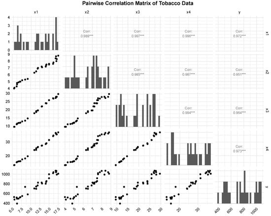
Figure 1. Correlation matrix of tobacco data. The color gradient and clustering pattern clearly highlight relationships and multicollinearity among predictors.

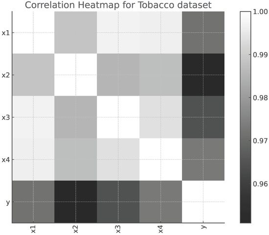
Figure 2. Correlation heatmap of tobacco data. The color gradient clearly highlight relationships and multicollinearity among predictors.

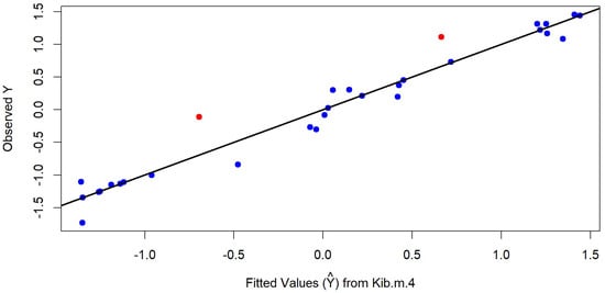
Figure 3. Diagnostic plot of KIB.M.4 estimator (observed vs. predicted values) using tobacco dataset.

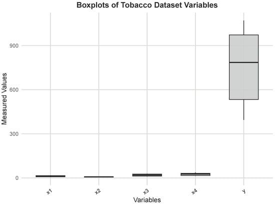
Figure 4. Boxplots of tobacco variables.

Table 15 presents the MSPEs comparison for the OLS, ridge-type (RR, HKB, and KIB1-KIB5), and proposed Kibria M-type estimators (KIB.M.1-KIB.M.5) based on the tobacco dataset. In particular, KIB.M.4 estimator yield the smallest MSPE value (1.6300), demonstrating improved performance in terms of both stability and predictive accuracy. Table 16 presents the (95%) confidence interval for tobacco dataset.

Table 15. MSPE comparison of OLS, ridge-type, and proposed Kibria M-estimators for the tobacco dataset.

Estimators	MSPE	${\widehat{\mathit{\beta }}}_1$	${\widehat{\mathit{\beta }}}_2$	${\widehat{\mathit{\beta }}}_3$	${\widehat{\mathit{\beta }}}_4$
OLS	1.7998	0.4857	−0.6728	1.0744	1.4438
RR	1.7241	0.4856	−0.6438	0.9563	1.0547
HKB	1.7114	0.4855	−0.6142	0.8510	0.8098
KIB1	4.3552	0.3674	−0.0091	0.0053	0.0024
KIB2	1.9615	0.4782	−0.1488	0.1004	0.0483
KIB3	8.4331	0.2520	−0.0032	0.0019	0.0008
KIB4	1.8243	0.4838	−0.3559	0.3112	0.1737
KIB5	19.5950	0.0961	−0.0007	0.0004	0.0002
M	1.7434	0.4888	−0.6500	1.2320	0.8844
KIB.M.1	3.3286	0.3793	−0.0098	0.0068	0.0016
KIB.M.2	1.7721	0.4839	−0.1976	0.1686	0.0447
KIB.M.3	8.3243	0.2537	−0.0031	0.0021	0.0005
KIB.M.4	1.6300	0.4876	−0.4122	0.4759	0.1542
KIB.M.5	19.5504	0.0968	−0.0007	0.0005	0.0001

Note: The bold value indicates the minimum MSPE among all estimators.

Table 16. Confidence interval bounds ($95\%$) for tobacco dataset.

Estimators	L(${\widehat{\mathit{\beta }}}_1$)	U(${\widehat{\mathit{\beta }}}_1$)	L(${\widehat{\mathit{\beta }}}_2$)	U(${\widehat{\mathit{\beta }}}_2$)	L(${\widehat{\mathit{\beta }}}_3$)	U(${\widehat{\mathit{\beta }}}_3$)	L(${\widehat{\mathit{\beta }}}_4$)	U(${\widehat{\mathit{\beta }}}_4$)
OLS	0.0059054	3.0088823	$-1.0815896$	0.0394569	$-1.9393480$	0.2561406	$-0.1586153$	1.8020345
RR	0.0867386	2.2906382	$-0.9925759$	0.0693685	$-1.4730159$	0.2829291	0.0020846	1.6677151
HKB	0.1370140	1.8385156	$-0.9152813$	0.0920081	$-1.1582346$	0.3073879	0.0938235	1.5392073
KIB.1	0.1716198	0.2039915	0.1572367	0.1920410	0.1663860	0.1994689	0.1729452	0.2059229
KIB.2	0.2426575	0.3705264	$-0.0233593$	0.2202691	0.1247362	0.3001765	0.2511665	0.4254661
KIB.3	0.1166258	0.1384949	0.1115066	0.1337473	0.1147861	0.1367611	0.1170717	0.1390304
KIB.4	0.2457064	0.6437700	$-0.3917211$	0.1852921	$-0.1416616$	0.3552923	0.2601261	0.7749550
KIB.5	0.0443078	0.0526219	0.0430615	0.0513997	0.0438667	0.0521876	0.0443933	0.0527132
M	0.0059054	3.0088823	$-1.0815896$	0.0394569	$-1.9393480$	0.2561406	$-0.1586153$	1.8020345
KIB.M.1	0.1763137	0.2096403	0.1602671	0.1965320	0.1704667	0.2046571	0.1777795	0.2118429
KIB.M.2	0.2463005	0.4289229	$-0.1201085$	0.2125613	0.0710544	0.3191113	0.2570068	0.5065816
KIB.M.3	0.1166566	0.1385315	0.1115348	0.1337816	0.1148159	0.1367969	0.1171028	0.1390674
KIB.M.4	0.2378959	0.7974902	$-0.5238798$	0.1683874	$-0.2935788$	0.3614426	0.2512087	0.9346472
KIB.M.5	0.0443085	0.0526228	0.0430622	0.0514006	0.0438674	0.0521885	0.0443941	0.0527141

5.2. Empirical Example-2: Anthropometric Data (Aged 2–19 Years)

To further evaluate the efficiency of the proposed estimators, we considered another real dataset titled “Anthropometric Data Aged 2–19”, which contains anthropometric measurements for individuals aged between 2 and 19 years. The dataset is available in Aslam, Muhammad (2020) [“Anthropometric-Data-Aged-2-19-Pak”, Mendeley Data, V1, doi: 10.17632/sxgymx5xjm.] and can be accessed from: https://data.mendeley.com/datasets/sxgymx5xjm/1 (accessed on 8 November 2025). The dataset includes the predictor variables like waist circumference (WC, cm), height for age (HpC, cm), mid–upper arm circumference (MUAC, cm), neck circumference (NC, cm), wrist circumference (WrC, cm), arm–to–height ratio (AHtR), waist–to–hip ratio (WHpR), waist–to–height ratio (WHtR), and hip–to–waist ratio (HWrR). The dependent variable is body mass index (BMI, kg/m²). To investigate the relationships among the predictors, a correlation matrix was constructed, and depicted in Figure 5. The figure clearly illustrates that the explanatory variables are highly correlated with one another, suggesting the presence of multicollinearity. The linear associations between the anthropometric variables in the dataset are visually shown by the correlation heatmap in Figure 6, which further confirms the presence of multicollinearity. The boxplot in Figure 7 further confirms the presence of extreme values in the dataset. Moreover, the estimated error variance for the anthropometric data was found to be $0.6077255$, which reflects a certain level of random variation or noise in the dataset. The corresponding eigenvalues are

$$\begin{array}{cc}\hfill {\lambda }_1& =4.3875, {\lambda }_2=1.7834, {\lambda }_3=1.1375, {\lambda }_4=0.7742,\hfill \\ \hfill {\lambda }_5& =0.5075, {\lambda }_6=0.3885, {\lambda }_7=0.0159,\hfill \\ \hfill {\lambda }_8& =0.0044, {\lambda }_9=0.0010.\hfill \end{array}$$

whereas the condition number of the anthropometric data is calculated as

$$C.N=\sqrt{{\displaystyle \frac{{\lambda }_{max}}{{\lambda }_{min}}}}=65.17221$$

which highlighting potential multicollinearity issues. Additionally, the condition number of the design matrix was $4247.417$, which far exceeds 1000, indicating that the matrix is severely ill-conditioned.

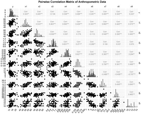
Figure 5. Correlation matrix of anthropometric variables (Aged 2–19). The color gradient and clustering pattern highlight relationships and multicollinearity among predictors (The correlation plot is based on standardized anthropometric data).

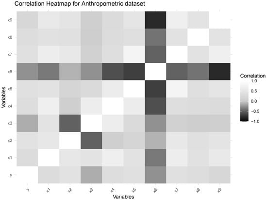
Figure 6. Correlation heatmap of anthropometric variables (aged 2–19). The color gradient highlights relationships and multicollinearity among predictors.

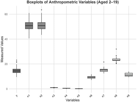
Figure 7. Boxplots of anthropometric variables (Aged 2–19). The points above the boxes represent potential outliers across the anthropometric measures (Data values are standardized for comparability).

Table 17 tabulates the MSPE values for the estimators used in this study. The proposed Kibria estimators (KIB.M.1–KIB.M.5) show improved performance over the traditional methods. These proposed estimators achieve notably lower MSPE values, suggesting that the incorporation of robust M-estimation principles enhances resistance to outlier influence and multicollinearity. Overall, the KIB.M.4 estimator yields the smallest MSPE ($68.2568$), implying improved predictive accuracy and robustness. These findings support the conclusion that the proposed Kibria M-estimators outperform both the OLS and standard ridge-type estimators in the anthropometric dataset, offering more reliable estimates of regression coefficients under model imperfections. Table 18 shows the 95% confidence interval of the anthropometric dataset.

Table 17. MSPE comparison of OLS, ridge-type, and proposed Kibria M-estimators for the anthropometric dataset.

Estimators	MSPE	${\widehat{\mathit{\beta }}}_1$	${\widehat{\mathit{\beta }}}_2$	${\widehat{\mathit{\beta }}}_3$	${\widehat{\mathit{\beta }}}_4$	${\widehat{\mathit{\beta }}}_5$	${\widehat{\mathit{\beta }}}_6$	${\widehat{\mathit{\beta }}}_7$	${\widehat{\mathit{\beta }}}_8$	${\widehat{\mathit{\beta }}}_9$
OLS	72.5852	0.2029	0.1626	−0.0777	0.0409	−0.3393	0.4497	−1.4793	−1.0506	1.6546
RR	70.9814	0.2028	0.1624	−0.0775	0.0407	−0.3379	0.4472	−1.2899	−0.7016	0.7677
HKB	69.9094	0.2025	0.1618	−0.0770	0.0404	−0.3343	0.4403	−0.9463	−0.3612	0.3046
KIB1	73.3716	0.1810	0.1263	−0.0490	0.0226	−0.1753	0.1923	−0.0408	−0.0087	0.0059
KIB2	70.9385	0.1945	0.1474	−0.0642	0.0317	−0.2542	0.3041	−0.1085	−0.0240	0.0165
KIB3	73.0660	0.1770	0.1207	−0.0455	0.0207	−0.1595	0.1720	−0.0339	−0.0072	0.0049
KIB4	70.3152	0.2004	0.1579	−0.0733	0.0378	−0.3098	0.3958	−0.3220	−0.0797	0.0565
KIB5	84.4507	0.0945	0.0438	−0.0119	0.0047	−0.0345	0.0329	−0.0044	−0.0009	0.0006
M	69.0314	0.2378	0.1261	−0.1219	0.0341	−0.2591	0.4571	−0.9687	−1.5091	0.4482
KIB.M.1	70.4580	0.2178	0.1035	−0.0843	0.0211	−0.1516	0.2269	−0.0349	−0.0165	0.0021
KIB.M.2	68.9276	0.2303	0.1171	−0.1053	0.0280	−0.2072	0.3365	−0.0926	−0.0457	0.0059
KIB.M.3	70.5320	0.2245	0.1106	−0.0947	0.0244	−0.1780	0.2766	−0.0532	−0.0254	0.0033
KIB.M.4	68.2568	0.2356	0.1233	−0.1165	0.0320	−0.2413	0.4135	−0.2562	−0.1448	0.0196
KIB.M.5	80.6594	0.1105	0.0339	−0.0186	0.0039	−0.0263	0.0334	−0.0029	−0.0013	0.0002

Note: The bold value indicates the minimum MSPE among all estimators.

Table 18. Confidence interval bounds (95%) for the anthropometric dataset.

Estimator	L(${\widehat{\mathit{\beta }}}_1$)	U(${\widehat{\mathit{\beta }}}_1$)	L(${\widehat{\mathit{\beta }}}_2$)	U(${\widehat{\mathit{\beta }}}_2$)	L(${\widehat{\mathit{\beta }}}_3$)	U(${\widehat{\mathit{\beta }}}_3$)	L(${\widehat{\mathit{\beta }}}_4$)	U(${\widehat{\mathit{\beta }}}_4$)	L(${\widehat{\mathit{\beta }}}_5$)	U(${\widehat{\mathit{\beta }}}_5$)	L(${\widehat{\mathit{\beta }}}_6$)	U(${\widehat{\mathit{\beta }}}_6$)	L(${\widehat{\mathit{\beta }}}_7$)	U(${\widehat{\mathit{\beta }}}_7$)	L(${\widehat{\mathit{\beta }}}_8$)	U(${\widehat{\mathit{\beta }}}_8$)	L(${\widehat{\mathit{\beta }}}_9$)	U(${\widehat{\mathit{\beta }}}_9$)
OLS	$-1.2015$	$3.3828$	$-2.6193$	$1.4454$	$-3.0770$	$0.8195$	$-1.1750$	$1.2864$	$-1.2387$	$0.3497$	$-2.4249$	$0.2535$	$-0.0969$	$1.5903$	$-0.0580$	$0.3311$	$-2.6133$	$0.0372$
RR	$-0.6232$	$1.5833$	$-1.1585$	$0.8401$	$-1.6648$	$0.2438$	$-0.5812$	$1.0923$	$-1.0807$	$0.2568$	$-1.7127$	$0.1139$	$-0.0014$	$1.4233$	$-0.0599$	$0.3184$	$-1.8943$	$-0.0835$
HKB	$-0.3123$	$0.6310$	$-0.3819$	$0.5042$	$-0.9133$	$-0.0657$	$-0.1057$	$0.8420$	$-0.7538$	$0.2325$	$-1.0044$	$0.0041$	$0.0255$	$1.0750$	$-0.0615$	$0.3092$	$-1.1821$	$-0.1721$
KIB1	$-0.0279$	$0.1115$	$0.1003$	$0.2476$	$-0.2233$	$-0.0716$	$0.0821$	$0.2425$	$0.0492$	$0.2122$	$-0.1240$	$0.0313$	$0.0038$	$0.1587$	$-0.0082$	$0.1963$	$-0.1575$	$-0.0017$
KIB2	$-0.0629$	$0.1254$	$0.1143$	$0.3121$	$-0.3254$	$-0.1191$	$0.1263$	$0.3671$	$0.0207$	$0.2644$	$-0.1871$	$0.0344$	$-0.0192$	$0.2234$	$-0.0365$	$0.2508$	$-0.2857$	$-0.0585$
KIB3	$-0.0216$	$0.1082$	$0.0955$	$0.2331$	$-0.2047$	$-0.0632$	$0.0742$	$0.2208$	$0.0497$	$0.1990$	$-0.1151$	$0.0281$	$0.0089$	$0.1499$	$-0.0032$	$0.1843$	$-0.1363$	$0.0066$
KIB4	$-0.1096$	$0.1681$	$0.0654$	$0.3514$	$-0.4549$	$-0.1636$	$0.1501$	$0.5163$	$-0.1479$	$0.2649$	$-0.3420$	$0.0023$	$-0.0089$	$0.4227$	$-0.0575$	$0.2868$	$-0.4910$	$-0.1369$
KIB5	$0.0116$	$0.0517$	$0.0360$	$0.0797$	$-0.0507$	$-0.0062$	$0.0209$	$0.0623$	$0.0268$	$0.0679$	$-0.0454$	$-0.0042$	$0.0233$	$0.0628$	$0.0162$	$0.0627$	$-0.0079$	$0.0326$
M	$-1.2015$	$3.3828$	$-2.6193$	$1.4454$	$-3.0770$	$0.8195$	$-1.1750$	$1.2864$	$-1.2387$	$0.3497$	$-2.4249$	$0.2535$	$-0.0969$	$1.5903$	$-0.0580$	$0.3311$	$-2.6133$	$0.0372$
KIB.M.1	$-0.0375$	$0.1158$	$0.1066$	$0.2677$	$-0.2511$	$-0.0844$	$0.0941$	$0.2757$	$0.0466$	$0.2303$	$-0.1383$	$0.0348$	$-0.0038$	$0.1726$	$-0.0160$	$0.2132$	$-0.1903$	$-0.0154$
KIB.M.2	$-0.0723$	$0.1300$	$0.1120$	$0.3244$	$-0.3532$	$-0.1316$	$0.1368$	$0.4012$	$-0.0006$	$0.2703$	$-0.2117$	$0.0298$	$-0.0210$	$0.2524$	$-0.0431$	$0.2618$	$-0.3252$	$-0.0766$
KIB.M.3	$-0.0526$	$0.1215$	$0.1131$	$0.2959$	$-0.2952$	$-0.1050$	$0.1135$	$0.3297$	$0.0356$	$0.2534$	$-0.1648$	$0.0365$	$-0.0144$	$0.1992$	$-0.0284$	$0.2369$	$-0.2454$	$-0.0399$
KIB.M.4	$-0.1242$	$0.1908$	$0.0381$	$0.3585$	$-0.4897$	$-0.1671$	$0.1433$	$0.5509$	$-0.2114$	$0.2596$	$-0.3962$	$-0.0055$	$-0.0028$	$0.4924$	$-0.0594$	$0.2912$	$-0.5516$	$-0.1509$
KIB.M.5	$0.0116$	$0.0517$	$0.0359$	$0.0795$	$-0.0505$	$-0.0061$	$0.0208$	$0.0621$	$0.0267$	$0.0678$	$-0.0453$	$-0.0042$	$0.0232$	$0.0627$	$0.0162$	$0.0626$	$-0.0078$	$0.0326$
KIB2	$-0.0629$	$0.1254$	$0.1143$	$0.3121$	$-0.3254$	$-0.1191$	$0.1263$	$0.3671$	$0.0207$	$0.2644$	$-0.1871$	$0.0344$	$-0.0192$	$0.2234$	$-0.0365$	$0.2508$	$-0.2857$	$-0.0585$
KIB3	$-0.0216$	$0.1082$	$0.0955$	$0.2331$	$-0.2047$	$-0.0632$	$0.0742$	$0.2208$	$0.0497$	$0.1990$	$-0.1151$	$0.0281$	$0.0089$	$0.1499$	$-0.0032$	$0.1843$	$-0.1363$	$0.0066$
KIB4	$-0.1096$	$0.1681$	$0.0654$	$0.3514$	$-0.4549$	$-0.1636$	$0.1501$	$0.5163$	$-0.1479$	$0.2649$	$-0.3420$	$0.0023$	$-0.0089$	$0.4227$	$-0.0575$	$0.2868$	$-0.4910$	$-0.1369$
KIB5	$0.0116$	$0.0517$	$0.0360$	$0.0797$	$-0.0507$	$-0.0062$	$0.0209$	$0.0623$	$0.0268$	$0.0679$	$-0.0454$	$-0.0042$	$0.0233$	$0.0628$	$0.0162$	$0.0627$	$-0.0079$	$0.0326$
M	$-1.2015$	$3.3828$	$-2.6193$	$1.4454$	$-3.0770$	$0.8195$	$-1.1750$	$1.2864$	$-1.2387$	$0.3497$	$-2.4249$	$0.2535$	$-0.0969$	$1.5903$	$-0.0580$	$0.3311$	$-2.6133$	$0.0372$
KIB.M.1	$-0.0375$	$0.1158$	$0.1066$	$0.2677$	$-0.2511$	$-0.0844$	$0.0941$	$0.2757$	$0.0466$	$0.2303$	$-0.1383$	$0.0348$	$-0.0038$	$0.1726$	$-0.0160$	$0.2132$	$-0.1903$	$-0.0154$
KIB.M.2	$-0.0723$	$0.1300$	$0.1120$	$0.3244$	$-0.3532$	$-0.1316$	$0.1368$	$0.4012$	$-0.0006$	$0.2703$	$-0.2117$	$0.0298$	$-0.0210$	$0.2524$	$-0.0431$	$0.2618$	$-0.3252$	$-0.0766$
KIB.M.3	$-0.0526$	$0.1215$	$0.1131$	$0.2959$	$-0.2952$	$-0.1050$	$0.1135$	$0.3297$	$0.0356$	$0.2534$	$-0.1648$	$0.0365$	$-0.0144$	$0.1992$	$-0.0284$	$0.2369$	$-0.2454$	$-0.0399$
KIB.M.4	$-0.1242$	$0.1908$	$0.0381$	$0.3585$	$-0.4897$	$-0.1671$	$0.1433$	$0.5509$	$-0.2114$	$0.2596$	$-0.3962$	$-0.0055$	$-0.0028$	$0.4924$	$-0.0594$	$0.2912$	$-0.5516$	$-0.1509$
KIB.M.5	$0.0116$	$0.0517$	$0.0359$	$0.0795$	$-0.0505$	$-0.0061$	$0.0208$	$0.0621$	$0.0267$	$0.0678$	$-0.0453$	$-0.0042$	$0.0232$	$0.0627$	$0.0162$	$0.0626$	$-0.0078$	$0.0326$

6. Conclusions

In this study, we explored the combined impact of multicollinearity and response-direction outliers on the performance of several classical and newly proposed estimators. It was observed that the traditional OLS and RR estimators do not perform efficiently in terms of the MSE when multicollinearity coexists with outliers in the response direction. Although robust M-estimators are generally employed to handle such issues, their performance deteriorates when severe multicollinearity and large error variance are present simultaneously. To overcome these limitations, five new modified Kibria M-estimators have been proposed.

Extensive Monte Carlo simulations indicate that the proposed estimators, particularly KIB.M.1, KIB.M.3, and KIB.M.5, outperform existing OLS, RR, and RM estimators by yielding lower MSE values across various levels of multicollinearity and data contamination. Additional simulations under heavy-tailed error distributions, specifically the standardized Cauchy distribution, further confirm the robustness of the proposed estimators. In this challenging scenario, where traditional estimators such as OLS, RR, and HKB produced extremely large MSEs due to the infinite variance of the Cauchy errors, the KIB.M estimators exhibited remarkable stability. Notably, KIB.M.5 tends to perform best, and achieved the lowest MSE across all configurations of sample size, number of predictors, and multicollinearity levels, highlighting its exceptional resilience to both multicollinearity and heavy-tailed noise. Furthermore, analyses of two real datasets, using MSPE criterion, demonstrate that the KIB.M estimators, particularly KIB.M.4, deliver the most stable and efficient estimates, outperforming all competing methods.

Future research may extend the proposed methodology in several directions. First, applying the proposed estimators to generalized linear models or high-dimensional settings would broaden their applicability. Second, developing adaptive data-driven approaches for optimal biasing parameter selection could enhance computational efficiency. Finally, exploring Bayesian or machine learning-based frameworks for robust ridge-type estimation may further improve robustness and predictive accuracy in the presence of complex data structures and severe multicollinearity.

References

- Frisch, R. Wirtschaftsrechnung und Input-Output-Analyse; G. Fischer Verlag: Jena, Germany, 1934. [Google Scholar]
- Belsley, D.A.; Kuh, E.; Welsch, R.E. Regression Diagnostics: Identifying Influential Data and Sources of Collinearity; John Wiley & Sons: Hoboken, NJ, USA, 2005. [Google Scholar]
- Hoerl, A.E.; Kennard, R.W. Ridge regression: Applications to nonorthogonal problems. Technometrics 1970, 12, 69–82. [Google Scholar] [CrossRef]
- Kibria, B.M.G. More than hundred (100) estimators for estimating the shrinkage parameter in a linear and generalized linear ridge regression models. J. Econom. Stat. 2022, 2, 233–252. [Google Scholar] [CrossRef]
- Khalaf, G.; Månsson, K.; Shukur, G. Modified ridge regression estimators. Commun. Stat.-Theory Methods 2013, 42, 1476–1487. [Google Scholar] [CrossRef]
- Dar, I.S.; Chand, S. New heteroscedasticity-adjusted ridge estimators in linear regression model. Commun. Stat.-Theory Methods 2024, 53, 7087–7101. [Google Scholar] [CrossRef]
- Gujarati, D.N.; Porter, D.C. Basic Econometrics, 5th ed.; McGraw-Hill Irwin: New York, NY, USA, 2009. [Google Scholar]
- Silvapulle, M.J. Robust ridge regression based on an M-estimator. Aust. J. Stat. 1991, 33, 319–333. [Google Scholar] [CrossRef]
- Ertaş, H. A modified ridge m-estimator for linear regression model with multicollinearity and outliers. Commun. Stat.-Simul. Comput. 2018, 47, 1240–1250. [Google Scholar] [CrossRef]
- Yasin, S.; Salem, S.; Ayed, H.; Kamal, S.; Suhail, M.; Khan, Y.A. Modified Robust Ridge M-Estimators in Two-Parameter Ridge Regression Model. Math. Probl. Eng. 2021, 2021, 1845914. [Google Scholar] [CrossRef]
- Majid, A.; Amin, M.; Aslam, M.; Ahmad, S. New robust ridge estimators for the linear regression model with outliers. Commun. Stat.-Simul. Comput. 2023, 52, 4717–4738. [Google Scholar] [CrossRef]
- Wasim, D.; Zaman, Q.; Ahmad, M.; Kibria, B.G. Mitigating multicollinearity and outliers in regression: Comparison of some new and old robust ridge M-estimators. J. Stat. Comput. Simul. 2025, 95, 3526–3547. [Google Scholar] [CrossRef]
- Alharthi, M.F. Novel Data-Driven Shrinkage Ridge Parameters for Handling Multicollinearity in Regression Models with Environmental and Chemical Data Applications. Axioms 2025, 14, 812. [Google Scholar] [CrossRef]
- Alharthi, M.F.; Akhtar, N. Newly Improved Two-Parameter Ridge Estimators: A Better Approach for Mitigating Multicollinearity in Regression Analysis. Axioms 2025, 14, 186. [Google Scholar] [CrossRef]
- Akhtar, N.; Alharthi, M.F.; Khan, M.S. Mitigating Multicollinearity in Regression: A Study on Improved Ridge Estimators. Mathematics 2024, 12, 3027. [Google Scholar] [CrossRef]
- Shah, I.; Sajid, F.; Ali, S.; Rehman, A.; Bahaj, S.A.; Fati, S.M. On the performance of jackknife based estimators for ridge regression. IEEE Access 2021, 9, 68044–68053. [Google Scholar] [CrossRef]
- Shaheen, N.; Shah, I.; Almohaimeed, A.; Ali, S.; Alqifari, H.N. Some modified ridge estimators for handling the multicollinearity problem. Mathematics 2023, 11, 2522. [Google Scholar] [CrossRef]
- Zhou, Q.; Cook, R.; Zou, G. Large sample properties of Huber M-estimators in linear regression models. J. Stat. Theory Pract. 2024, 18, 45–68. [Google Scholar]
- Montgomery, D.C.; Peck, E.A.; Vining, G.G. Introduction to Linear Regression Analysis; John Wiley & Sons: Hoboken, NJ, USA, 2021. [Google Scholar]
- Huber, P.J.; Ronchetti, E.M. Robust Statistics; John Wiley & Sons: Hoboken, NJ, USA, 2011. [Google Scholar]
- Ertaş, A. A Robust Ridge M-Estimator for the Linear Regression Model. Commun. Stat.-Simul. Comput. 2018, 47, 2938–2949. [Google Scholar] [CrossRef]
- Hoerl, A.E.; Kannard, R.W.; Baldwin, K.F. Ridge regression: Some simulations. Commun. Stat.-Theory Methods 1975, 4, 105–123. [Google Scholar] [CrossRef]
- McDonald, G.C.; Galarneau, D.I. A Monte Carlo evaluation of some ridge-type estimators. J. Am. Stat. Assoc. 1975, 70, 407–416. [Google Scholar] [CrossRef]
- McDonald, R.P. Handbook of Multivariate Experimental Psychology, 2nd ed.; Springer: New York, NY, USA, 2009. [Google Scholar] [CrossRef]
- Majid, M.; Danish, M.; Haq, S.U.; Naz, H. A robust two-parameter ridge estimator for handling multicollinearity and heteroscedasticity. Commun. Stat.-Simul. Comput. 2021, 50, 2581–2595. [Google Scholar] [CrossRef]
- Suhail, M.; Chand, S.; Kibria, B.G. Quantile-based robust ridge m-estimator for linear regression model in presence of multicollinearity and outliers. Commun. Stat.-Simul. Comput. 2021, 50, 3194–3206. [Google Scholar] [CrossRef]
- Shabbir, M.; Chand, S.; Iqbal, F. A new ridge estimator for linear regression model with some challenging behavior of error term. Commun. Stat.-Simul. Comput. 2024, 53, 5442–5452. [Google Scholar] [CrossRef]
- Rousseeuw, P.J. Robust estimation and identifying outliers. Handb. Stat. Methods Eng. Sci. 1990, 16, 11–16. [Google Scholar]
Disclaimer/Publisher’s Note: The statements, opinions and data contained in all publications are solely those of the individual author(s) and contributor(s) and not of MDPI and/or the editor(s). MDPI and/or the editor(s) disclaim responsibility for any injury to people or property resulting from any ideas, methods, instructions or products referred to in the content. |
© 2025 by the authors. Licensee MDPI, Basel, Switzerland. This article is an open access article distributed under the terms and conditions of the Creative Commons Attribution (CC BY) license (https://creativecommons.org/licenses/by/4.0/).