Korovkin-Type Approximation Theorems for Statistical Gauge Integrable Functions of Two Variables

Abstract

In this work, we develop and investigate statistical extensions of gauge integrability and gauge summability for double sequences of functions of two real variables, formulated within the framework of deferred weighted means. We begin by establishing several fundamental limit theorems that serve to connect these generalized notions and provide a rigorous theoretical foundation. Based on these results, we establish Korovkin-type approximation theorems using the classical test function set $1,s,t,s^2+t^2$ in the Banach space $\mathcal{C}\left({[0,1]}^2\right)$. To demonstrate the applicability of the proposed framework, we further present an example involving families of positive linear operators associated with the Meyer-König and Zeller (MKZ) operators. These findings not only extend classical Korovkin-type theorems to the setting of statistical deferred gauge integrability and summability but also underscore their robustness in addressing double sequences and the approximation of two-variable functions.

1. Introduction

The theory of integration has undergone a remarkable evolution, progressing from the classical Riemann integral to the more flexible and powerful gauge (Henstock–Kurzweil) integral [1]. The Riemann integral, introduced in the 19th century, provided a rigorous foundation for integration by partitioning intervals and summing rectangular areas. While adequate for many classical problems, it faced significant limitations, particularly in dealing with functions exhibiting highly oscillatory behavior or lacking uniform continuity.

Lebesgue addressed these limitations with his measure-theoretic integral [1], broadening the scope of integrability and laying the foundation for modern analysis. However, in certain approximation contexts requiring finer local control, even the Lebesgue integral proved restrictive. This led to the development of the gauge (Henstock–Kurzweil) integral, independently formulated by Henstock and Kurzweil in the mid-20th century. Unlike the Riemann and Lebesgue integrals, it utilizes variable meshes guided by gauge functions, enabling the integration of functions with discontinuities and irregular oscillations that were previously non-integrable.

The gauge integral significantly advanced approximation theory, providing a natural pathway for extending Korovkin-type theorems, which serve as fundamental tools for establishing the convergence of sequences of positive linear operators. The original Korovkin theorem, formulated for continuous functions of a single variable, introduced a minimal set of test functions for verifying uniform convergence. Building on gauge integrability, these results were subsequently generalized to broader univariate settings and later to multivariate functions, including double and multiple sequences of operators.

In higher dimensions, particularly for bivariate and multivariate operators, the gauge integral has proven highly effective in addressing convergence phenomena that lie beyond the reach of classical methods. Moreover, the interplay between gauge integration and Korovkin-type approximation has opened new avenues for studying statistical convergence, deferred summability, and weighted means in both univariate and multivariate frameworks.

Thus, the historical journey from Riemann to gauge integration reflects both a deepening of integration theory and its profound impact on modern approximation theory, extending Korovkin-type results from classical univariate settings to versatile frameworks involving several variables and double sequences.

Motivated by the above-mentioned investigation and study, we introduce the historical development of integration theory from the Riemann and Lebesgue integrals to the more flexible Henstock–Kurzweil (gauge) integral, emphasizing its advantages in handling oscillatory and discontinuous functions. It highlights how gauge integration naturally extends Korovkin-type approximation theorems to multivariable settings and provides finer control in convergence studies. However, the paper could strengthen its introduction by explicitly identifying the research gap that existing Korovkin-type results for double sequences have not yet been formulated within the framework of statistical gauge integrability and summability using deferred weighted means.

2. Methods

Let $I:=[a,b]$ and $J:=[c,d]$ be two non-degenerate compact intervals on $\mathbb{R}$, with $a<b$ and $c<d$. The Cartesian product

$$\begin{array}{c}\hfill R:=I\times J=[a,b]\times [c,d]\end{array}$$

defines a compact rectangle in ${\mathbb{R}}^2$. A partition $\mathcal{P}$ of R is a finite collection of non-overlapping sub-rectangles

$$\begin{array}{c}\hfill \mathcal{P}:={\left\{R_{ij}\right\}}_{i=1,j=1}^{m,n},\end{array}$$

such that

$$\begin{array}{c}\hfill R=\bigcup _{i=1}^m\bigcup _{j=1}^n{R}_{ij}.\end{array}$$

Each sub-rectangle $R_{ij}$ has the form

$$\begin{array}{c}\hfill R_{ij}=[x_{i-1},x_i]\times [y_{j-1},y_j],\end{array}$$

where the partitions of the intervals are given by

$$\begin{array}{c}\hfill a=x_0<x_1<\cdots <x_m=b,c=y_0<y_1<\cdots <y_n=d.\end{array}$$

Thus, the rectangle R is subdivided into $m\times n$ smaller rectangles, arranged so that adjacent subintervals align properly along both axes.

The lengths of the intervals are denoted by

$$\begin{array}{c}\hfill \ell \left(I\right)=b-a,\ell \left(J\right)=d-c,\end{array}$$

with $\ell \left(I\right),\ell \left(J\right)\ge 0$. Clearly, $\ell \left(I\right)=0$ if and only if $a=b$, and $\ell \left(J\right)=0$ if and only if $c=d$. In such degenerate cases, the corresponding rectangle R collapses to a line segment or a point in ${\mathbb{R}}^2$. Otherwise, when both $\ell \left(I\right)$ and $\ell \left(J\right)$ are positive, R has a nontrivial area

$$\begin{array}{c}\hfill \ell \left(R\right)=\ell \left(I\right)·\ell \left(J\right)=(b-a)(d-c),\end{array}$$

which represents the extent of the region covered in the plane.

Consider a rectangle $R=[a,b]\times [c,d]$ in ${\mathbb{R}}^2$, and let

$$\begin{array}{c}\hfill \mathcal{P}={\left\{R_{ij}\right\}}_{i=1,j=1}^{m,n}\end{array}$$

be a partition of R, where each sub-rectangle is of the form

$$\begin{array}{c}\hfill R_{ij}=[x_{i-1},x_i]\times [y_{j-1},y_j],\end{array}$$

with

$$\begin{array}{c}\hfill a=x_0<x_1<\cdots <x_m=b,c=y_0<y_1<\cdots <y_n=d.\end{array}$$

For each sub-rectangle $R_{ij}$, we associate a point $(t_i,s_j)\in R_{ij}$, which is referred to as the tag of $R_{ij}$. Such a construction is called a tagged partition of R, and is often represented as

$$\begin{array}{c}\hfill \dot{\mathcal{P}}=\{(R_{ij},(t_i,s_j)):i=1,2,\dots ,m,j=1,2,\dots ,n\}.\end{array}$$

We now define the mesh (or norm) of $\dot{\mathcal{P}}$ is defined by

$$\begin{array}{c}\hfill \parallel \dot{\mathcal{P}}\parallel :=\underset{i,j}{max}\{diam\left(R_{ij}\right)\},\end{array}$$

where $diam\left(R_{ij}\right)=max\{x_i-x_{i-1},y_j-y_{j-1}\}$. This notion is used in the Riemann-style definitions that require uniformly fine partitions.

In other words, a tagged partition of R consists of ordered pairs $\left\{(R_{ij},(t_i,s_j))\right\}$, where $\left\{R_{ij}\right\}$ forms a partition of R, and $(t_i,s_j)$ is the chosen tag of the corresponding sub-rectangle. It is clear that a given partition admits infinitely many possible tagged versions, since the tags can be chosen arbitrarily within each sub-rectangle.

We define the notion of the Riemann sum in the bivariate case, let $\left\{g_{m,n}\right\}$ be a double sequence of functions defined on $R=[a,b]\times [c,d]$, and let $\dot{\mathcal{P}}$ be a tagged partition of R. The corresponding Riemann sum is defined as

$$\begin{array}{c}\hfill R(g_{m,n};\dot{\mathcal{P}})(x,y):=\sum _{i=1}^m\sum _{j=1}^n{g}_{i,j}(t_i,s_j)\ell \left(R_{ij}\right),\end{array}$$

where

$$\begin{array}{c}\hfill \ell \left(R_{ij}\right)=(x_i-x_{i-1})(y_j-y_{j-1})\end{array}$$

denotes the area of the sub-rectangle $R_{ij}$.

Definition 1.

Let $R=[a,b]\times [c,d]\subset {\mathbb{R}}^2$ be a compact rectangle. A double sequence of functions $\left\{g_{m,n}\right\}$ defined on R is said to be Riemann integrable over R with limit function g, if for all $(x,y)\in R,$ and for every $ϵ>0$ there exists a number ${\gamma }_{ϵ}>0$ such that for any tagged partition

$$\begin{array}{c}\hfill \dot{\mathcal{P}}=\{(R_{ij},(t_i,s_j)):i=1,2,\dots ,m,j=1,2,\dots ,n\}\end{array}$$

of R, with

$$\begin{array}{c}\hfill \underset{i,j}{max}\{\ell \left(R_{ij}\right)\}\le {\gamma }_{ϵ},\end{array}$$

the corresponding Riemann sum satisfies

$$\begin{array}{c}\hfill |\mathcal{R}(g_{m,n};\dot{\mathcal{P}})(x,y)-g(x,y)|\le ϵ,\end{array}$$

where

$$\begin{array}{c}\hfill \mathcal{R}(g_{m,n};\dot{\mathcal{P}})(x,y):=\sum _{i=1}^m\sum _{j=1}^n{g}_{i,j}(t_i,s_j)\ell \left(R_{ij}\right),\ell \left(R_{ij}\right)=(x_i-x_{i-1})(y_j-y_{j-1}).\end{array}$$

The fundamental significance of the Riemann integral for a double sequence of functions $\left\{g_{m,n}\right\}$ defined on the rectangle $R=[a,b]\times [c,d]\subset {\mathbb{R}}^2$ lies in its interpretation as the limit of the associated double Riemann sums. As the tagged partitions of R become progressively finer in both variables, the corresponding sums converge in an appropriate manner to the integral value.

The key objective of this article is to move beyond the traditional Riemann framework for defining the limit of double Riemann sums associated with a sequence of functions. Instead, we adopt a generalized limit process, independently introduced by the Czech mathematician Kurzweil [1] and the English mathematician Henstock [1]. Although this approach is technically more involved than the classical Riemann procedure, it provides a broader and more versatile notion of integration. In particular, it significantly enlarges the class of integrable double sequences of functions defined on rectangles in ${\mathbb{R}}^2$. Moreover, the method is more flexible and convenient, as it circumvents certain restrictive assumptions inherent in the Riemann theory. Thus, with only a modest increase in technical complexity, one obtains a powerful and refined integral concept, representing a noteworthy advancement in integration theory.

In the classical Riemann approach, the fineness of a partition of a rectangle $R=[a,b]\times [c,d]$ is determined by the mesh, defined as the maximum length of the subintervals in both directions. Accordingly, each sub-rectangle must have side lengths smaller than or equal to a prescribed tolerance. In contrast, the Kurzweil–Henstock methodology [1] allows partitions with highly variable sub-rectangle sizes. In this framework, sub-rectangles in regions where the function exhibits rapid oscillations or steep gradients are chosen to be sufficiently small, while in regions of slower variation, larger sub-rectangles may be employed. This local adaptability makes the Kurzweil–Henstock integral particularly well-suited for double sequences of functions, providing a natural and refined approach to integration in two variables.

In 1957, the Czech mathematician Kurzweil [1] introduced a new formulation of the integral that remained faithful to Riemann’s original framework. A few years later, in 1961, the English mathematician Henstock [1] independently developed a similar construction, thereby extending the scope of the classical Riemann integral. Their contributions together gave rise to what is now known as the Henstock–Kurzweil (HK) integral [1], a powerful generalization of the Riemann integral that has since played a significant role in modern integration theory.

In the case of functions of two variables defined over a rectangular domain

$$\begin{array}{c}\hfill R=[a,b]\times [c,d],\end{array}$$

the Henstock–Kurzweil integral emphasizes the role of tags more prominently than the traditional Riemann framework. Specifically, for a tagged double partition

$$\begin{array}{c}\hfill \dot{\mathcal{P}}=\left\{([x_{i-1},x_i]\times [y_{j-1},y_j],(t_i,s_j)):1\le i\le m,1\le j\le n\right\},\end{array}$$

the fineness of the partition is not governed merely by the uniform length of subrectangles. Instead, each subrectangle is required to lie within a gauge neighborhood of its tag, namely

$$\begin{array}{c}\hfill \mathcal{G}[(t_i,s_j);{\delta }_{i,j}]=[t_i-{\delta }_{i,j},t_i+{\delta }_{i,j}]\times [s_j-{\delta }_{i,j},s_j+{\delta }_{i,j}],\end{array}$$

where ${\delta }_{i,j}>0$ may vary from one tag to another.

This flexible control on partitions allows the HK integral in two variables (and hence for double sequences of functions) to integrate a far broader class of functions than the classical Riemann method, particularly those with local irregularities or oscillations.

We begin by introducing the following definitions:

Definition 2.

Let $R=[a,b]\times [c,d]\subset {\mathbb{R}}^2$ be a compact rectangle. A mapping $\delta :R\to (0,\infty )$ is called a gauge on R if, $\delta (t,s)>0$ for every $(t,s)\in R$. For each $(t,s)\in R$, the gauge δ determines the neighborhood

$$\begin{array}{c}\hfill \mathcal{G}\left[\right(t,s);\delta ]=[t-\delta (t,s),t+\delta (t,s\left)\right]\times [s-\delta (t,s),s+\delta (t,s\left)\right],\end{array}$$

which is referred to as the gauge interval centered at $(t,s)$. In the setting of double sequences of functions, such gauge neighborhoods provide the essential mechanism for regulating the fineness of tagged double partitions of R.

Definition 3.

Let $R=[a,b]\times [c,d]\subset {\mathbb{R}}^2$ be a compact rectangle, and let

$$\begin{array}{c}\hfill \dot{\mathcal{P}}=\{(R_{ij},(t_i,s_j)):i=1,2,\dots ,m,j=1,2,\dots ,n\}\end{array}$$

denotes a tagged partition of R, where each sub-rectangle is given by $R_{ij}=[x_{i-1},x_i]\times [y_{j-1},y_j]$, and $(t_i,s_j)\in R_{ij}$ is its corresponding tag.

If $\delta :R\to (0,\infty )$ is a gauge on R, then the tagged partition $\dot{\mathcal{P}}$ is called $\delta$-fine if, for every pair of indices $i=1,2,\dots ,m$ and $j=1,2,\dots ,n$, the sub-rectangle $R_{ij}$ is contained within the gauge neighborhood

$$\begin{array}{c}\hfill R_{ij}\subseteq [t_i-\delta (t_i,s_j),t_i+\delta (t_i,s_j)]\times [s_j-\delta (t_i,s_j),s_j+\delta (t_i,s_j)].\end{array}$$

In other words, each sub-rectangle $R_{ij}$ must be entirely contained within the gauge interval determined by its tag $(t_i,s_j)$.

In view of the above definitions we present an illustrative example below.

Example 1.

Consider the rectangle $R=[0,1]\times [0,1]\subset {\mathbb{R}}^2$.

• Define a gauge function $\delta :R\to (0,\infty )$ by

  $$\begin{array}{c}\hfill \delta (t,s)=\frac{1}{4}min\{t+1,s+1\}.\end{array}$$

We partition $R=[0,1]\times [0,1]$ into four equal sub-rectangles,

$$\begin{array}{c}\hfill R_{11}=[0,\frac{1}{2}]\times [0,\frac{1}{2}],R_{12}=[0,\frac{1}{2}]\times [\frac{1}{2},1],\end{array}$$

$$\begin{array}{c}\hfill R_{21}=[\frac{1}{2},1]\times [0,\frac{1}{2}],R_{22}=[\frac{1}{2},1]\times [\frac{1}{2},1].\end{array}$$

The tags $(t_i,s_j)$ are chosen as the midpoints of each sub-rectangle, namely,

$$\begin{array}{c}\hfill (t_1,s_1)=(\frac{1}{4},\frac{1}{4}),(t_1,s_2)=(\frac{1}{4},\frac{3}{4}),(t_2,s_1)=(\frac{3}{4},\frac{1}{4}),(t_2,s_2)=(\frac{3}{4},\frac{3}{4}).\end{array}$$

Now, consider the sub-rectangle $R_{11}=[0,\frac{1}{2}]\times [0,\frac{1}{2}]$.

For the tag $(t_1,s_1)=(\frac{1}{4},\frac{1}{4})$, we compute

$$\begin{array}{c}\hfill \delta (t_1,s_1)=\frac{1}{4}min\{\frac{1}{4}+1,\frac{1}{4}+1\}=\frac{1}{4}·\frac{5}{4}=\frac{5}{16}.\end{array}$$

Thus, the corresponding gauge interval is

$$\begin{array}{c}\hfill [t_1-\delta (t_1,s_1),t_1+\delta (t_1,s_1)]\times [s_1-\delta (t_1,s_1),s_1+\delta (t_1,s_1)]=[-\frac{1}{16},\frac{9}{16}]\times [-\frac{1}{16},\frac{9}{16}].\end{array}$$

Since $R_{11}=[0,\frac{1}{2}]\times [0,\frac{1}{2}]\subseteq [-\frac{1}{16},\frac{9}{16}]\times [-\frac{1}{16},\frac{9}{16}]$, the δ-fine condition holds for this sub-rectangle. A similar verification shows that the condition also holds for $R_{12}$, $R_{21}$, and $R_{22}$.

Therefore, the tagged partition

$$\begin{array}{c}\hfill \dot{\mathcal{P}}=\{(R_{ij},(t_i,s_j)):i,j=1,2\}\end{array}$$

is δ-fine.

We now proceed to define the gauge integral (also known as the generalized Riemann integral) in the setting of a double sequence of functions $\left\{g_{m,n}\right\}$ defined on a rectangular domain of ${\mathbb{R}}^2$.

Consider a double sequence of functions $\left\{g_{m,n}\right\}$ defined on the compact rectangle $I\times J=[a,b]\times [c,d]\subset {\mathbb{R}}^2$. Let

$$\begin{array}{c}\hfill \dot{\mathcal{P}}={\left\{(R_{i,j},(t_i,s_j))\right\}}_{i=1,j=1}^{m,n}\end{array}$$

denotes a tagged partition of $I\times J$, where each $R_i$ is a sub-rectangle of $I\times J$ and $(t_i,s_j)\in R_{i,j}$ serves as its tag.

If $\delta :I\times J\to (0,\infty )$ is a gauge, then the tagged partition $\dot{\mathcal{P}}$ is said to be δ-fine whenever

$$\begin{array}{c}\hfill R_{i,j}\subseteq \left[t_i-\delta (t_i,s_j),t_i+\delta (t_i,s_j)\right]\times \left[s_j-\delta (t_i,s_j),s_i+\delta (t_i,s_j)\right],\forall i=1,2,\dots ,m,j=1,2,\dots ,n.\end{array}$$

The corresponding gauge sum of the double sequence $\left\{g_{m,n}\right\}$ with respect to the tagged partition $\dot{\mathcal{P}}$ is defined

$$\begin{array}{c}\hfill \mathcal{G}(g_{m,n};\dot{\mathcal{P}})(x,y):=\sum _{i=1}^m\sum _{j=1}^n{g}_{i,j}(t_i,s_j)\ell \left(R_{i,j}\right),\end{array}$$

where $\ell \left(R_{i,j}\right)$ denotes the area (Lebesgue measure) of the sub-rectangle $R_{i,j}$.

Definition 4.

A double sequence of functions $\left(g_{m,n}\right)$ is said to be gauge integrable (or generalized Riemann integrable) over the compact rectangle $I\times J=[a,b]\times [c,d]\subset {\mathbb{R}}^2$ if there exists a function $g(x,y)$ such that for every $ϵ>0$ there is a gauge ${\delta }_{ϵ}$ defined on $I\times J$ with the following property:

For any tagged partition

$$\begin{array}{c}\hfill \dot{\mathcal{P}}={\left\{(R_{i,j},(t_i,s_j))\right\}}_{i=1,j=1}^{m,n}\end{array}$$

of $I\times J$ that is ${\delta }_{ϵ}$-fine, the corresponding gauge sum satisfies

$$\begin{array}{c}\hfill \left|\mathcal{G}(g_{m,n};\dot{\mathcal{P}})(x,y)-g(x,y)\right|\le ϵ,\end{array}$$

where

$$\begin{array}{c}\hfill \mathcal{G}(g_{m,n};\dot{\mathcal{P}})(x,y):=\sum _{i=1}^m\sum _{j=1}^n{g}_{i,j}(t_i,s_j)\ell \left(R_{i,j}\right),\end{array}$$

and $\ell \left(R_{i,j}\right)$ denotes the area of the sub-rectangle $R_{i,j}$.

The following example illustrates the evaluation of the Kurzweil–Henstock (or gauge) integral of $g_{m,n}$ over ${[0,1]}^2$ with respect to a tagged partition $\dot{\mathcal{P}}$.

Example 2.

Consider a double sequence of bivariate functions $\left\{g_{m,n}(x,y)\right\}$ defined on the compact domain $[0,1]\times [0,1]$ by

$$\begin{array}{c}\hfill g_{m,n}(x,y)=e^{-(x+y)}+{\displaystyle \frac{1}{m}}sin\left(2\pi x\right)cos\left(2\pi y\right)+{\displaystyle \frac{1}{n}}cos\left(3\pi x\right)sin\left(2\pi y\right),(x,y)\in [0,1]\times [0,1],\end{array}$$

where $m,n\in \mathbb{N}$.

The corresponding limit function of this double sequence is

$$g(x,y)=\underset{m,n\to \infty }{lim}{g}_{m,n}(x,y)=e^{-(x+y)}.$$

Each function $g_{m,n}(x,y)$ represents a smooth oscillatory perturbation of the limit function, with the perturbation amplitude decreasing as $m,n\to \infty$.

The gauge (or control) function $\delta (x,y;m,n)$, which determines the adaptive tagged partition of the domain, is defined by

$$\begin{array}{c}\hfill \delta (x,y;m,n)=0.12+0.08\left({sin}^2\left(2\pi x\right)+{sin}^2\left(2\pi y\right)\right)+0.02\left({\displaystyle \frac{1}{m}}+{\displaystyle \frac{1}{n}}\right),\end{array}$$

for all $(x,y)\in [0,1]\times [0,1]$.

The gauge takes smaller values in regions of higher oscillation (for instance, near the center of the domain) and larger values in flatter regions. Consequently, the domain $[0,1]\times [0,1]$ is subdivided into rectangles $R_{ij}$ satisfying

$$diam\left(R_{ij}\right)\le max\{x_i-x_{i-1},y_j-y_{j-1}\}.$$

We denote the Kurzweil–Henstock (or gauge) double integral of $g_{m,n}(x,y)$ by

$$I_{m,n}={\int }_0^1{\int }_0^1{g}_{m,n}(x,y)dxdy.$$

(1)

It follows that

$$\underset{m,n\to \infty }{lim}{I}_{m,n}=I_{\mathrm{exact}};$$

that is, the double sequence of integrals $\left\{I_{m,n}\right\}$ converges uniformly to the exact integral of the limit function $g(x,y)$.

Moreover, the double integral of the limit function $g(x,y)$ over the unit square $[0,1]\times [0,1]$ is given by

$$I_{\mathrm{exact}}={\int }_0^1{\int }_0^1{e}^{-(x+y)}dxdy={(1-e^{-1})}^2.$$

(2)

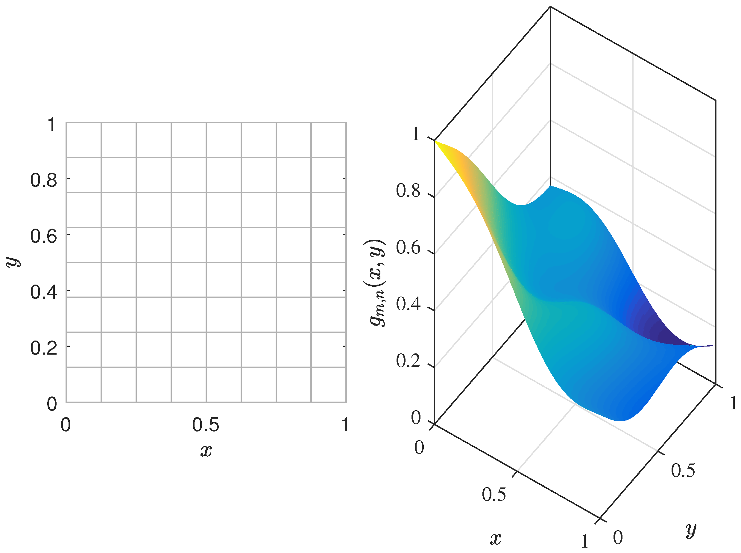
In view of Example 2, we use MATLAB R2016b visualization (Figure 1) to illustrate the geometric interpretation and convergence behavior of the gauge-tagged partition for $g_{m,n}(x,y)$.

Figure 1. Gauge-tagged partition $\dot{\mathcal{P}}$ (left) and $g_{m,n}(x,y)$ (right).

The left panel of Figure 1 shows how the Kurzweil–Henstock (gauge) integral divides the domain ${[0,1]}^2$ into smaller parts in an adaptive way. In regions where the function changes quickly or oscillates more, the rectangles automatically become smaller according to the gauge function $\delta (x,y;m,n)$. The parameters m and n control how much the function oscillates and how smooth it is. Unlike the classical Riemann method, which uses subintervals of equal size, the gauge method allows variable sizes, making it more flexible for handling irregular functions while still achieving convergence. The right panel of Figure 1 shows the function $g_{m,n}(x,y)$ for a specific pair $(m,n)$, helping to compare the function’s oscillations with the corresponding adaptive partition. Together, the two panels show that stronger oscillations lead to finer partitions, which is the main idea behind the Kurzweil–Henstock (gauge) approach.

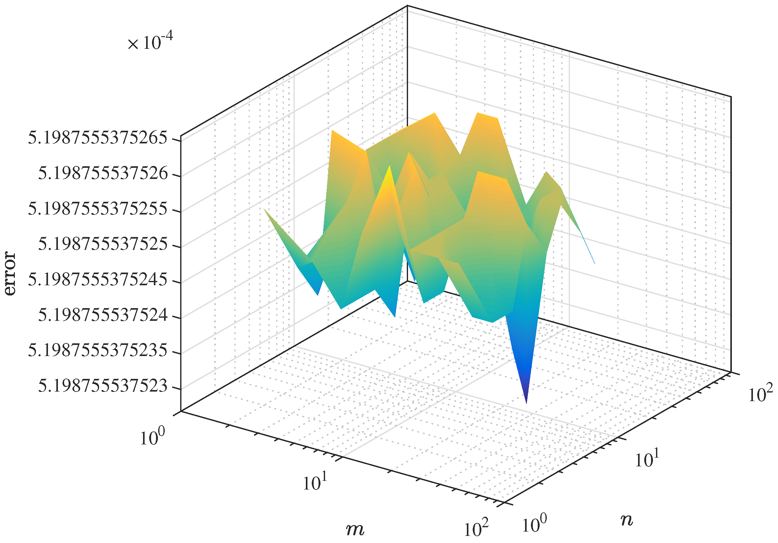
Figure 2 shows the surface plot of the absolute integration error $|I_{m,n}-I_{\mathrm{exact}}|$ for different values of m and n. This Figure 2 illustrates how the numerical results get closer to the exact value of the integral as both m and n increase. Here,

$$I_{m,n}={\int \int }_{{\displaystyle {[0,1]}^2}}{g}_{m,n}(x,y)dxdy$$

represents the numerical estimate of the two-dimensional Kurzweil–Henstock (gauge) integral for the function $g_{m,n}(x,y)$, and

$$I_{\mathrm{exact}}={\int }_0^1{\int }_0^1{e}^{-(x+y)}dxdy={(1-e^{-1})}^2$$

is the exact analytical value of the same integral.

Figure 2. Error surface $|I_{m,n}-I_{\mathrm{exact}}|$.

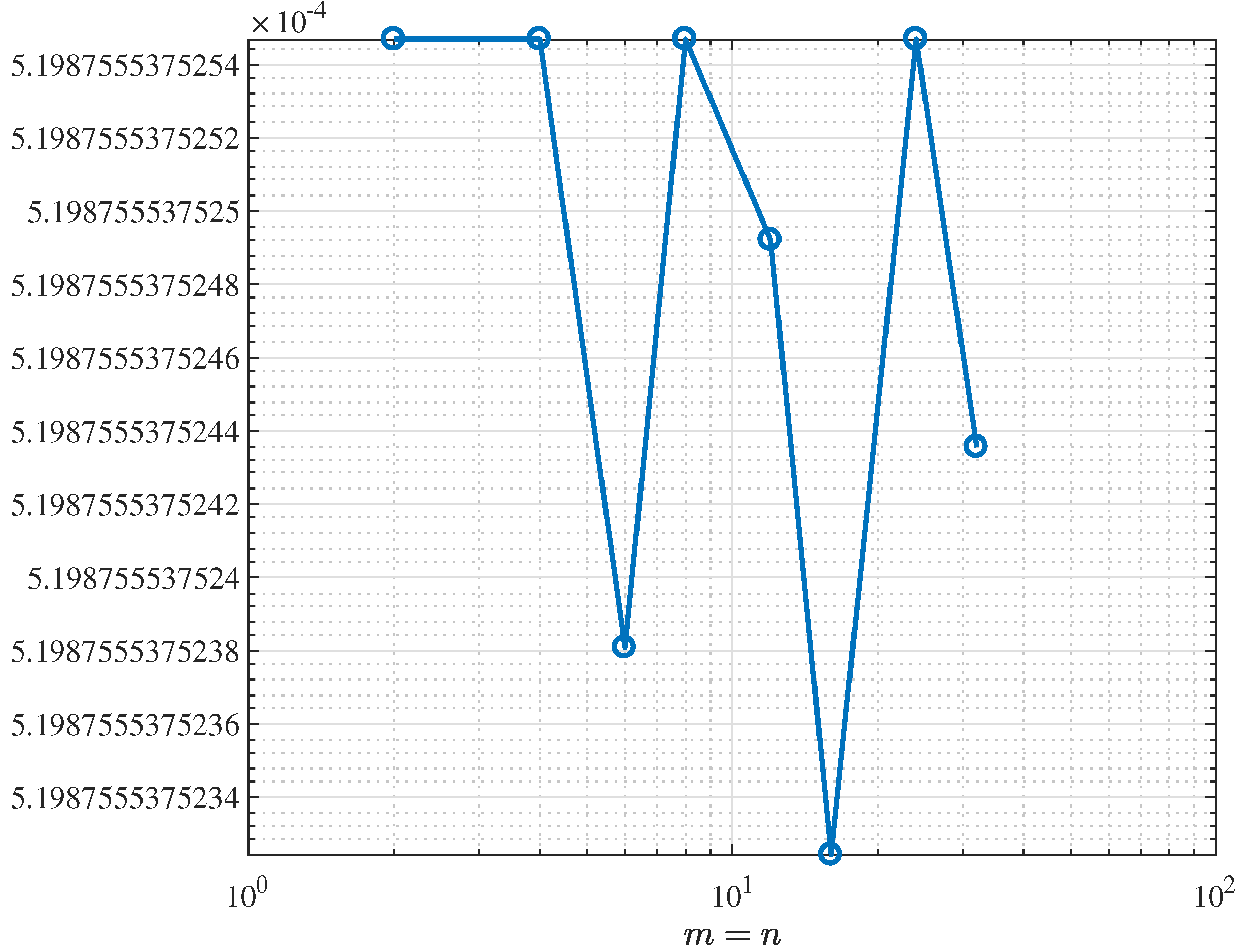
Figure 3 shows how the results converge when m and n are taken to be equal (that is, $m=n$). Both axes are shown on a logarithmic scale, so a straight line in the plot indicates a power-law rate of convergence. By focusing on the case $m=n$, the figure gives a simpler one-dimensional view of the convergence, instead of the full two-dimensional error surface. This makes it easier to estimate how fast the double sequence converges along its diagonal and to compare the observed numerical behavior with any available theoretical error bounds.

Figure 3. Convergence of $g_{m,n}(x,y)$ along $m=n$.

The classical theory of convergence forms the backbone of sequence space analysis, providing a rigorous foundation for approximation and summability methods. Building on this framework, Fast [2] and Steinhaus [3] independently introduced statistical convergence, a powerful generalization of ordinary convergence that has since become an essential tool for both theoretical investigations and diverse applications.

In particular, the study of statistical convergence for double sequences of functions of two variables has developed into a powerful extension, offering a flexible framework for investigating approximation processes and summability methods. Its importance lies not only in its theoretical richness but also in its wide applicability across various branches of mathematics. In fact, it establishes strong links with engineering mathematics, computational mathematics, industrial mathematics, and financial mathematics, thereby underscoring its growing role in both theoretical research and real-world applications.

The vitality of this research area is further reflected in numerous recent contributions (see, for example, [4,5,6,7,8,9,10,11,12]), which demonstrate the depth and breadth of statistical convergence and its generalizations in the context of double sequences.

Definition 5.

A double sequence ${\left(u_{m,n}\right)}_{m,n\in \mathbb{N}}$ is said to be statistically convergent to a limit α if, for every $ϵ>0$, the proportion of terms of the sequence that deviate from α by at least ϵ becomes negligible as both indices m and n tend to infinity. Equivalently, the set of index pairs

$$\begin{array}{c}\hfill \{(m,n)\in \mathbb{N}\times \mathbb{N}:|u_{m,n}-\alpha |\ge ϵ\}\end{array}$$

has natural density zero.

Formally, this condition is expressed as

$$\begin{array}{c}\hfill \underset{M,N\to \infty }{lim}{\displaystyle \frac{1}{MN}}\left|\{(m,n):1\le m\le M,1\le n\le N,|u_{m,n}-\alpha |\ge ϵ\}\right|=0.\end{array}$$

Thus, if a double sequence $\left(u_{m,n}\right)$ is statistically convergent to α, we write

$$\begin{array}{c}\hfill stat\underset{m,n\to \infty }{lim}{u}_{m,n}=\alpha .\end{array}$$

In 2021, Srivastava et al. [13] established a connection between statistically Riemann-integrable double sequences of functions, denoted $\mathrm{RI}\mathrm{stat}$, and statistically limit-integrable sequences, denoted $\mathrm{stat}\mathrm{LI}$, thereby proving Korovkin-type approximation theorems in this framework. This line of research was extended in 2022, when Srivastava et al. [14] derived additional Korovkin-type results for deferred weighted statistically Riemann-integrable sequences.

Further developments include the work of Jena and Paikray [15], who introduced a framework for statistical Riemann-Stieltjes integration and established several foundational results. Jena et al. [16] subsequently examined statistical Riemann integrability and summability under deferred Cesàro means, while Parida et al. [17] advanced the theory by studying deferred weighted statistically Riemann-summable sequences and formulating fuzzy Korovkin-type approximation theorems, thereby extending classical results to a broader and more flexible setting.

These contributions have inspired numerous generalizations, highlighting the richness of the subject. For further perspectives, one may consult [16,18,19,20,21,22,23,24,25,26,27], where various aspects of approximation theory, summability, and applications are explored in depth. Collectively, these works underscore both the historical development and the modern vitality of Korovkin-type results in diverse mathematical contexts.

In continuation of this line of research, we introduce two further notions for functions of two variables: statistically Riemann-integrable sequences, denoted $\mathrm{RI}\mathrm{stat}$, and statistically gauge-integrable sequences, denoted $\mathrm{GI}\mathrm{stat}$. The former provides a natural extension of the classical Riemann integral under statistical convergence in two dimensions, while the latter situates statistical integrability within the flexible Henstock–Kurzweil (gauge) framework. Together, these concepts extend classical integrability to the realm of double sequences, capture behaviors inaccessible to traditional approaches, and lay the groundwork for new Korovkin-type approximation theorems with broader applications in approximation theory and summability analysis.

Definition 6.

Let $\left\{g_{m,n}\right\}$ be a double sequence of functions defined on the rectangle $I\times J=[a,b]\times [c,d]$. We say that $\left\{g_{m,n}\right\}$ is statistically Riemann integrable (denoted by ${\mathrm{RI}}_{\mathrm{stat}}$) to a function g over $I\times J$ if, for every $ϵ>0$ and for all $(x,y)\in I\times J$, there exists a number ${\gamma }_{ϵ}>0$ such that, for every tagged partition $\dot{\mathcal{P}}={\left\{(R_{i,j},(t_i,s_i))\right\}}_{i=1,j=1}^{m,n}$ of $I\times J$ with mesh size $\parallel \dot{\mathcal{P}}\parallel <{\gamma }_{ϵ}$, the set

$$\begin{array}{c}\hfill {\mathfrak{E}}_{ϵ}=\left\{(m,n)\in {\mathbb{N}}^2:|R(g_{mn};\dot{\mathcal{P}})(x,y)-g(x,y)|\ge ϵ\right\}\end{array}$$

has natural density zero in ${\mathbb{N}}^2$. Formally, this means

$$\begin{array}{c}\hfill d\left({\mathfrak{E}}_{ϵ}\right)=\underset{M,N\to \infty }{lim}{\displaystyle \frac{1}{MN}}\left|\{(m,n)\le (M,N):(m,n)\in {\mathfrak{E}}_{ϵ}\}\right|=0.\end{array}$$

In this case, we denote the statistical Riemann integrability of $\left\{g_{m,n}(x,y)\right\}$ by

$$\begin{array}{c}\hfill {\mathrm{RI}}_{\mathrm{stat}}R(g_{m,n};\dot{\mathcal{P}})(x,y)=g(x,y)\mathrm{as}m,n\to \infty .\end{array}$$

Definition 7.

Let $\left\{g_{m,n}\right\}$ be a double sequence of functions defined on the rectangle $I\times J=[a,b]\times [c,d]$. We say that $\left\{g_{m,n}\right\}$ is statistically gauge integrable (denoted by ${\mathrm{GI}}_{\mathrm{stat}}$) to a function g over $I\times J$ if, for every $ϵ>0$, and for all $(x,y)\in I\times J$ there exists a gauge ${\delta }_{ϵ}$ defined on $I\times J$ such that, for every ${\delta }_{ϵ}$-fine tagged partition

$$\begin{array}{c}\hfill \dot{\mathcal{P}}={\left\{(R_{i,j},(t_i,s_i))\right\}}_{i=1,j=1}^{m,n}\end{array}$$

of $I\times J$, the set

$$\begin{array}{c}\hfill {\mathfrak{E}}_{ϵ}=\left\{(m,n)\in {\mathbb{N}}^2:|\mathcal{G}(g_{m,n};\dot{\mathcal{P}})(x,y)-g(x,y)|\ge ϵ\right\}\end{array}$$

has natural density zero in ${\mathbb{N}}^2$. Formally, this condition is expressed as

$$\begin{array}{c}\hfill d\left({\mathfrak{E}}_{ϵ}\right)=\underset{M,N\to \infty }{lim}{\displaystyle \frac{1}{MN}}\left|\{(m,n)\le (M,N):(m,n)\in {\mathfrak{E}}_{ϵ}\}\right|=0.\end{array}$$

In this case, the statistical gauge integrability of $\left\{g_{m,n}(x,y)\right\}$ is denoted by

$$\begin{array}{c}\hfill {\mathrm{GI}}_{\mathrm{stat}}\underset{m,n\to \infty }{lim}\mathcal{G}(g_{m,n};\dot{\mathcal{P}})(x,y)=g(x,y).\end{array}$$

The following theorem establishes a rigorous connection between the two concepts introduced above, namely statistical Riemann integrability and statistical gauge integrability, in the framework of double sequences of bivariate functions on the rectangle $[a,b]\times [c,d]$.

Theorem 1 (Connection between RIstat and GIstat).

Let $\left\{g_{m,n}\right\}$ be a double sequence of real-valued functions defined on the rectangle $I\times J=[a,b]\times [c,d]$, and let $g:I\times J\to \mathbb{R}$. Then the following hold:

 (a) 

If $\left\{g_{m,n}\right\}$ is statistically Riemann integrable to $g(x,y)$, then it is also statistically gauge integrable to $g(x,y)$.

 (b) 

Conversely, if $\left\{g_{m,n}\right\}$ is statistically gauge integrable to $g(x,y)$, and $g(x,y)$ is classically Riemann integrable, then $\left\{g_{m,n}\right\}$ is statistically Riemann integrable to $g(x,y)$.

Proof. 

(a) Let $\epsilon >0$ be given. By the definition of statistical Riemann integrability (${\mathrm{RI}}_{\mathrm{stat}}$), there exists a mesh threshold ${\gamma }_{\epsilon }>0$ such that for any tagged partition $\dot{\mathcal{P}}$ of $I\times J$ with mesh $\parallel \dot{\mathcal{P}}\parallel <{\gamma }_{\epsilon }$, the Riemann sums $\mathcal{R}(g_{m,n};\dot{\mathcal{P}})$ satisfy

$$|\mathcal{R}(g_{m,n};\dot{\mathcal{P}})(x,y)-g(x,y)|<\epsilon$$

for all $(m,n)$ except possibly on a subset of ${\mathbb{N}}^2$ of natural density zero.

Now, define a constant gauge on $I\times J$ by

$${\delta }_{\epsilon }(x,y)\equiv {\displaystyle \frac{{\gamma }_{\epsilon }}{2}}.$$

For any ${\delta }_{\epsilon }$-fine tagged partition, the mesh $\parallel \dot{\mathcal{P}}\parallel$ is bounded above by ${\gamma }_{\epsilon }$, hence every ${\delta }_{\epsilon }$-fine partition satisfies the same small-mesh condition required by ${\mathrm{RI}}_{\mathrm{stat}}$.

Therefore, the Riemann estimate immediately extends to the corresponding gauge sums,

$$|\mathcal{G}(g_{m,n};\dot{\mathcal{P}})(x,y)-g(x,y)|<\epsilon ,$$

again for all $(m,n)$ outside a subset of ${\mathbb{N}}^2$ of density zero. Moreover, the exceptional index set for the gauge integral is contained in the Riemann-exceptional set, which also has density zero. Hence, $g_{m,n}$ is ${\mathrm{GI}}_{\mathrm{stat}}$ whenever it is ${\mathrm{RI}}_{\mathrm{stat}}$.

(b) Conversely, assume that $g_{m,n}$ is ${\mathrm{GI}}_{\mathrm{stat}}$ with respect to the limit function g. Then, for each $\epsilon >0$, there exists a gauge ${\delta }_{\epsilon }$ such that for every ${\delta }_{\epsilon }$-fine tagged partition $\dot{\mathcal{P}}$ of $I\times J$,

$$|\mathcal{G}(g_{m,n};\dot{\mathcal{P}})(x,y)-g(x,y)|<{\displaystyle \frac{\epsilon }{2}}$$

for all $(m,n)$ except possibly on a subset of density zero.

Since $g(x,y)$ is Riemann integrable on $I\times J$, there exists ${\eta }_{\epsilon }>0$ such that for any tagged partition $\dot{\mathcal{P}}$ with mesh $\parallel \dot{\mathcal{P}} \parallel <{\eta }_{\epsilon }$, there is a ${\delta }_{\epsilon }$-fine refinement $\widehat{\mathcal{P}}$ satisfying

$$|\mathcal{R}(g_{m,n};\dot{\mathcal{P}})(x,y)-\mathcal{G}(g_{m,n};\widehat{\mathcal{P}})(x,y)|<{\displaystyle \frac{\epsilon }{2}}.$$

Using the triangle inequality, we obtain

$$\begin{array}{cc}\hfill |\mathcal{R}(g_{m,n};\dot{\mathcal{P}})(x,y)-g(x,y)|& \le |\mathcal{R}(g_{m,n};\dot{\mathcal{P}})(x,y)-\mathcal{G}(g_{m,n};\widehat{\mathcal{P}})(x,y)|\hfill \\ \hfill & +|\mathcal{G}(g_{m,n};\widehat{\mathcal{P}})(x,y)-g(x,y)|\hfill \\ \hfill & <{\displaystyle \frac{\epsilon }{2}}+{\displaystyle \frac{\epsilon }{2}}=\epsilon .\hfill \end{array}$$

The second term is controlled by the ${\mathrm{GI}}_{\mathrm{stat}}$ property, and the first by the closeness of Riemann and gauge sums for fine enough partitions. Thus, the ${\mathrm{RI}}_{\mathrm{stat}}$ condition is satisfied, establishing the equivalence between statistical Riemann and statistical gauge integrability. □

The following example demonstrates that, within the framework of double sequences of functions of two variables, the converse of Theorem 1 does not hold in general.

Example 3.

Let $R=[0,1]\times [0,1]$. Define the function

$$\begin{array}{c}\hfill g(x,y):={\mathbf{1}}_{{\mathbb{Q}}^2\cap R}(x,y)=\left\{\begin{array}{cc}1,\hfill & (x,y)\in {\mathbb{Q}}^2\cap R,\hfill \\ 0,\hfill & \text{otherwise},\hfill \end{array}\right.\end{array}$$

where ${\mathbb{Q}}^2=\mathbb{Q}\times \mathbb{Q}$.

Since the set of rational points ${\mathbb{Q}}^2\cap R$ has Lebesgue measure zero, it follows that g is Lebesgue integrable on R with ${\displaystyle {\int }_{R}g=0}$. Consequently, g is Henstock–Kurzweil (gauge) integrable on R, and its gauge integral equals 0. On the other hand, g is discontinuous at every point of R (since every rectangle contains both rational and irrational points). Therefore, g is not Riemann integrable on R, as Riemann integrability requires the set of discontinuities to have measure zero.

For each $m,n\in \mathbb{N}$, define

$$\begin{array}{c}\hfill g_{m,n}(x,y):=g(x,y)\mathit{for}\mathit{all}(x,y)\in R.\end{array}$$

Thus $\left\{g_{m,n}\right\}$ is the constant double sequence with each term equal to g.

Since g is gauge integrable on R with integral 0, for every $ϵ>0$ there exists a gauge ${\delta }_{ϵ}$ on R such that every ${\delta }_{ϵ}$-fine tagged partition $\dot{\mathcal{P}}$ satisfies

$$\begin{array}{c}\hfill \left|\mathcal{G}\right(g;\dot{\mathcal{P}})-0|<ϵ.\end{array}$$

For the constant sequence $g_{m,n}\equiv g$ the gauge sums $\mathcal{G}(g_{m,n};\dot{\mathcal{P}})$ coincide with $\mathcal{G}(g;\dot{\mathcal{P}})$ for every $(m,n)$. Hence, for this ${\delta }_{ϵ}$ and for every ${\delta }_{ϵ}$-fine partition the exceptional index set

$$\begin{array}{c}\hfill {\mathfrak{E}}_{ϵ}=\left\{(m,n)\in {\mathbb{N}}^2:|\mathcal{G}(g_{m,n};\dot{\mathcal{P}})-0|\ge ϵ\right\}\end{array}$$

is empty, and therefore has natural density zero. This confirms that

$$\begin{array}{c}\hfill {\mathrm{GI}}_{\mathrm{stat}}\underset{m,n\to \infty }{lim}\mathcal{G}(g_{m,n};\dot{\mathcal{P}})=0.\end{array}$$

Take $ϵ=\frac{1}{2}$. For any mesh threshold $\gamma >0$, tagged partitions with all tags chosen from rational points, and similarly, there exist γ-fine partitions with all tags chosen from irrational points. For a partition consisting solely of rational tags, the corresponding Riemann sum satisfies $\mathcal{R}(g;\dot{\mathcal{P}})=1$, whereas for a partition consisting solely of irrational tags, we obtain $\mathcal{R}(g;\dot{\mathcal{P}})=0$. Thus, no single number L can serve as a Riemann limit approximating all γ-fine Riemann sums simultaneously.

In particular, for the constant sequence $g_{m,n}=g$ and the chosen ϵ, there exist γ-fine partitions $\dot{\mathcal{P}}$ for which the exceptional index set

$$\begin{array}{c}\hfill {\mathfrak{E}}_{ϵ}=\left\{(m,n)\in {\mathbb{N}}^2:|\mathcal{R}(g_{m,n};\dot{\mathcal{P}})-L|\ge ϵ\right\}\end{array}$$

coincides with the whole of ${\mathbb{N}}^2$ (and hence of density 1) for every putative limit L. Therefore, the sequence $\left\{g_{m,n}\right\}$ does not satisfy the ${\mathrm{RI}}_{\mathrm{stat}}$ condition.

This example demonstrates that a double sequence may be statistically gauge integrable to a function g (in this case with gauge integral equal to 0) while failing to be statistically Riemann integrable. Thus, the converse implication in Theorem 1 does not hold, in general, without additional assumptions, such as the classical Riemann integrability of g.

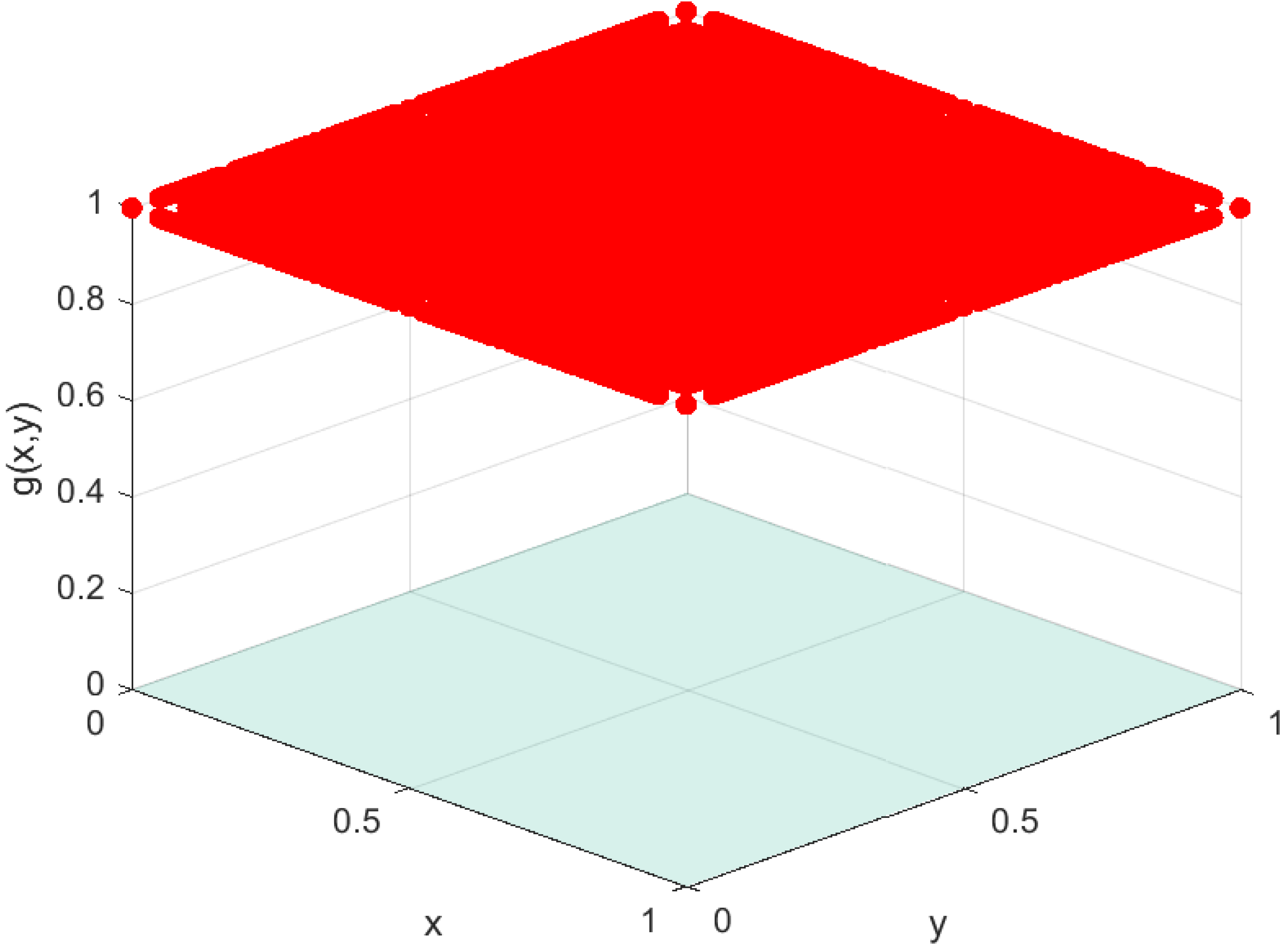
To gain further insight into Example 3, Figure 4 presents a three-dimensional visualization of $g(x,y)$. Its significance may be interpreted as follows:

Figure 4. 3D visualization of $g(x,y)$ with Riemann sum 1 (for rational) and 0 for (irrational).

(i)

Red Scatter Points ($z=1$): The red points represent the rational points $(x,y)$ with denominators bounded by a fixed constant. At these points, the function value is $g(x,y)=1$. Since the rationals are dense in $[0,1]\times [0,1]$, these red points appear throughout the square, even though they form only a countable set.

(ii)

Transparent Blue/Gray Plane ($z=0$): The surface at height zero corresponds to all irrational points. At these points, the function is defined as $g(x,y)=0$. Since the irrationals are uncountable and dense in $[0,1]\times [0,1]$, this plane dominates the region, showing that the function is “almost everywhere zero.”

(iii)

Overall Interpretation: The juxtaposition of isolated red points above a continuous plane at $z=0$ highlights the dual nature of the function. The density of rationals causes the red points to scatter across the entire region, but their measure is zero. Thus, the integral is governed entirely by the blue/gray plane at $z=0$. This provides a visual explanation of why the function is not Riemann integrable in the classical sense, yet can be treated effectively within the gauge or statistical integration frameworks.

Motivated by the above body of work and the recent developments in this area, we aim to broaden the scope of analysis by investigating the notions of gauge integrability and gauge summability within the statistical framework for double sequences of functions. In particular, we incorporate deferred weighted summability methods, which allow for a more flexible treatment of convergence phenomena. Our first goal is to formulate and prove a collection of fundamental limit theorems that reveal intrinsic connections between these enriched concepts of summability and integrability. Building upon this foundation, we then establish Korovkin-type approximation theorems for functions of two variables with respect to the standard test functions 1, s, t, and $s^2+t^2$. To demonstrate the practical significance of these abstract results, we conclude by presenting an illustrative example involving a family of positive linear operators associated with the well-known Meyer-König and Zeller operators, thereby underscoring the effectiveness and applicability of our proposed theoretical framework in approximation theory.

Gauge Integrability via Deferred Weighted Mean

Let $\left(a_m\right)$, $\left(b_m\right)$, $\left(c_n\right)$, $\left(d_n\right)$ be sequences in ${\mathbb{Z}}^{0+}$ such that

$$a_m<b_m,c_n<d_n,\underset{m\to \infty }{lim}{b}_m=\underset{n\to \infty }{lim}{d}_n=+\infty .$$

Suppose $\left\{p_{i,j}\right\}$ is a double sequence of nonnegative weights and define the cumulative weight

$$P_{m,n}=\sum _{i=a_m+1}^{b_m}\sum _{j=c_n+1}^{d_n}{p}_{i,j}(m,n\in \mathbb{N}),$$

with $P_{m,n}>0$ sufficiently large $(m,n)$.

Let $\left\{g_{i,j}\right\}$ be a double sequence of functions on a rectangle $R=I\times J$ and let $\dot{\mathcal{P}}$ be a tagged partition of R. The deferred weighted gauge mean of the gauge sums $\mathcal{G}(g_{i,j};\dot{\mathcal{P}})$ over the delayed index rectangle $[a_m+1,b_m]\times [c_n+1,d_n]$ is defined by

$$W_{m,n}\left(\mathcal{G}(g_{i,j};\dot{\mathcal{P}})\right)={\displaystyle \frac{1}{P_{m,n}}}\sum _{i=a_m+1}^{b_m}\sum _{j=c_n+1}^{d_n}{p}_{i,j}\mathcal{G}\left(g_{i,j};\dot{\mathcal{P}}\right).$$

(3)

Here $\mathcal{G}(g_{i,j};\dot{\mathcal{P}})$ denotes the gauge sum of the function $g_{i,j}$ with respect to the tagged partition $\dot{\mathcal{P}}$, and $W_{m,n}(·)$ represents the deferred weighted average of these gauge sums over the index window $(i,j)\in [a_m+1,b_m]\times [c_n+1,d_n]$. The weight under double-sum allows flexible emphasis on particular indices and naturally extends single-index deferred weighted means to the double-sequence setting.

We now proceed to introduce the notions of statistical gauge integrability and statistical gauge summability for double sequences of functions in two variables. These concepts are developed within the framework of deferred weighted summability means, thereby providing a refined extension of classical integrability and summability techniques to the statistical setting. This formulation not only generalizes existing approaches but also establishes a versatile foundation for the study of approximation processes in the context of functions of two variables.

Definition 8.

Let $\left(a_m\right)$, $\left(b_m\right)$, $\left(c_n\right)$, and $\left(d_n\right)$ be sequences in ${\mathbb{Z}}^{0+}$ satisfying $a_m<b_m$ and $c_n<d_n$. Consider also a double sequence $\left(p_{m,n}\right)$ in

$$\begin{array}{c}\hfill {\mathbb{R}}_{*}^2:=\left({\mathbb{R}}^{+}\cup \left\{0\right\}\right)\times \left({\mathbb{R}}^{+}\cup \left\{0\right\}\right).\end{array}$$

A double sequence of functions $\left\{g_{m,n}\right\}$ is said to be statistically deferred weighted gauge integrable (${\mathrm{DWG}}_{\mathrm{stat}}$) to a function $g(x,y)$ over the rectangle $[a,b]\times [c,d]$ if, for every $ϵ>0$, there exists a corresponding gauge ${\delta }_{ϵ}$ such that for any ${\delta }_{ϵ}$-fine tagged partition

$$\begin{array}{c}\hfill \dot{\mathcal{P}}={\left\{(R_{ij},(x_i,y_j))\right\}}_{i,j=1}^{m,n}\end{array}$$

of $[a,b]\times [c,d]$, the exceptional index set

$$\begin{array}{c}\hfill {\mathfrak{E}}_{ϵ}=\left\{(\mu ,\nu )\le P_{m,n}:p_{\mu ,\nu }|\mathcal{G}(g_{\mu ,\nu };\dot{\mathcal{P}})(x,y)-g(x,y)|\ge ϵ\right\}\end{array}$$

has double natural density zero. Equivalently, for each $ϵ>0$,

$$\begin{array}{c}\hfill \underset{m,n\to \infty }{lim}{\displaystyle \frac{\left|\right\{(\mu ,\nu )\leqq P_{m,n}:p_{\mu ,\nu }|\mathcal{G}(g_{\mu ,\nu };\dot{\mathcal{P}})(x,y)-g(x,y)|\geqq ϵ\left\}\right|}{P_{m,n}}}=0.\end{array}$$

In this case, we write

$$\begin{array}{c}\hfill {\mathrm{DWG}}_{\mathrm{stat}}\underset{m,n\to \infty }{lim}\mathcal{G}(g_{m,n};\dot{\mathcal{P}})(x,y)=g(x,y).\end{array}$$

Definition 9.

Let $\left(a_m\right)$, $\left(b_m\right)$, $\left(c_n\right)$, and $\left(d_n\right)$ be sequences in ${\mathbb{Z}}^{0+}$ satisfying $a_m<b_m$ and $c_n<d_n$. Further, let $\left(p_{m,n}\right)$ be a double sequence in

$$\begin{array}{c}\hfill {\mathbb{R}}_{*}^2:=\left({\mathbb{R}}^{+}\cup \left\{0\right\}\right)\times \left({\mathbb{R}}^{+}\cup \left\{0\right\}\right).\end{array}$$

A double sequence of functions $\left\{g_{m,n}\right\}$ is said to be statistically deferred weighted gauge summable (denoted ${\mathrm{stat}}_{\mathrm{DWG}}$) to a function $g(x,y)$ over the rectangle $[a,b]\times [c,d]$ if, for every $ϵ>0$, one can find a gauge ${\delta }_{ϵ}$ such that, for any ${\delta }_{ϵ}$-fine tagged partition

$$\begin{array}{c}\hfill \dot{\mathcal{P}}={\left\{(R_{ij},(x_i,y_j))\right\}}_{i,j=1}^{m,n}\end{array}$$

of $[a,b]\times [c,d]$, the exceptional set

$$\begin{array}{c}\hfill {\mathfrak{E}}_{ϵ}=\left\{(\mu ,\nu )\le (m,n):|W\left(\mathcal{G}(g_{\mu ,\nu };\dot{\mathcal{P}})(x,y)\right)-g(x,y)|\ge ϵ\right\}\end{array}$$

has natural double density zero. Equivalently, for each $ϵ>0$,

$$\begin{array}{c}\hfill \underset{m,n\to \infty }{lim}{\displaystyle \frac{\left|\right\{(\mu ,\nu )\leqq (m,n):|W\left(\mathcal{G}(g_{\mu ,\nu };\dot{\mathcal{P}})(x,y)\right)-g(x,y)|\geqq ϵ\left\}\right|}{mn}}=0.\end{array}$$

In this case, we write

$$\begin{array}{c}\hfill {\mathrm{stat}}_{\mathrm{DWG}}\underset{m,n\to \infty }{lim}\mathcal{G}(g_{m,n};\dot{\mathcal{P}})(x,y)=g(x,y).\end{array}$$

We now turn to an inclusion theorem that reveals the intrinsic connection between the two recently introduced notions: statistical deferred weighted integrability and statistical deferred weighted gauge summability, both considered in the setting of double sequences. This result not only clarifies the interplay between these concepts but also emphasizes their potential relevance within the broader framework of approximation theory.

Theorem 2.

Let $\left\{g_{m,n}\right\}$ be a double sequence of real-valued functions on the rectangle $R=[a,b]\times [c,d]$. Suppose $\left\{p_{m,n}\right\}$ is a double sequence of nonnegative weights and, for each $(m,n)$, $P_{m,n}={\sum }_{i=a_m+1}^{b_m}{\sum }_{j=c_n+1}^{d_n}{p}_{i,j}>0$ for all sufficiently large $m,n$. Then

$$\begin{array}{c}\hfill {\mathrm{DWG}}_{\mathrm{stat}}\text{-}\mathrm{integrability}\mathrm{of}\left\{g_{m,n}\right\}⟹{\mathrm{stat}}_{\mathrm{DWG}}\text{-}\mathrm{summability}\mathrm{of}\left\{g_{m,n}\right\},\end{array}$$

That is, if $\left\{g_{m,n}\right\}$ is statistically deferred weighted gauge integrable to a limit function $g(x,y)$ on R, then the deferred weighted gauge means of the gauge sums converge statistically to the same limit function $g(x,y)$ on R. In general, however, the converse implication does not hold.

Proof. 

Assume $\left\{g_{m,n}\right\}$ is ${\mathrm{DWG}}_{\mathrm{stat}}$-integrable to $g(x,y)$ on R. Fix $ϵ>0$. By the definition of ${\mathrm{DWG}}_{\mathrm{stat}}$-integrability there exists a gauge ${\delta }_{ϵ}$ and an associated ${\delta }_{ϵ}$-fine tagged partition $\dot{\mathcal{P}}$ of R such that the exceptional index set

$$\begin{array}{c}\hfill {\mathfrak{E}}_{ϵ}:=\left\{(i,j)\in [a_m+1,b_m]\times [c_n+1,d_n]:p_{i,j}|\mathcal{G}(g_{i,j};\dot{\mathcal{P}})-g|\ge ϵ\right\}\end{array}$$

has deferred weighted double density tending to zero. In other words, for sufficiently large $m,n$ the proportion of indices in ${\mathfrak{E}}_{ϵ},$ measured with respect to the total weight, becomes negligible, i.e.,

$$\begin{array}{c}\hfill {\displaystyle \frac{1}{P_{m,n}}}\sum _{(i,j)\in {\mathfrak{E}}_{ϵ}}{p}_{i,j}=0(m,n\to \infty ).\end{array}$$

For the same partition $\dot{\mathcal{P}}$, define the deferred weighted gauge mean (see (3)) by

$$\begin{array}{c}\hfill W_{m,n}:={\displaystyle \frac{1}{P_{m,n}}}\sum _{i=a_m+1}^{b_m}\sum _{j=c_n+1}^{d_n}{p}_{i,j}\mathcal{G}(g_{i,j};\dot{\mathcal{P}}).\end{array}$$

Splitting the double sum into the contribution from the exceptional set ${\mathfrak{E}}_{ϵ}$ and from its complement, we obtain

$$\begin{array}{c}\hfill W_{m,n}-g(x,y)={\displaystyle \frac{1}{P_{m,n}}}\left(\sum _{(i,j)\notin {\mathfrak{E}}_{ϵ}}{p}_{i,j}\left(\mathcal{G}(g_{i,j};\dot{\mathcal{P}})-g\right)+\sum _{(i,j)\in {\mathfrak{E}}_{ϵ}}{p}_{i,j}\left(\mathcal{G}(g_{i,j};\dot{\mathcal{P}})(x,y)-g(x,y)\right)\right).\end{array}$$

By construction, if $(i,j)\notin {\mathfrak{E}}_{ϵ}$ then

$$|\mathcal{G}(g_{i,j};\dot{\mathcal{P}})-g|<ϵ/p_{i,j}$$

in the weighted formulation. However, a simpler uniform estimate follows directly from integrability. Since each $\mathcal{G}(g_{i,j};\dot{\mathcal{P}})$ is finite and g is fixed, there exists a global finite bound M such that $\left|\mathcal{G}\right(g_{i,j};\dot{\mathcal{P}})-g|\le M$ for all relevant $(i,j)$. Hence, we obtain

$$\begin{array}{c}\hfill \left|{\displaystyle \frac{1}{P_{m,n}}}\sum _{(i,j)\notin {\mathfrak{E}}_{ϵ}}{p}_{i,j}\left(\mathcal{G}(g_{i,j};\dot{\mathcal{P}})(x,y)-g(x,y)\right)\right|\le {\displaystyle \frac{1}{P_{m,n}}}\sum _{(i,j)\notin {\mathfrak{E}}_{ϵ}}{p}_{i,j}M\le M.\end{array}$$

Moreover, the contribution of the exceptional set is controlled by the definition of ${\mathrm{DWG}}_{\mathrm{stat}}$. For large $m,n$,

$$\begin{array}{c}\hfill \left|{\displaystyle \frac{G}{1}}{P}_{m,n}\sum _{(i,j)\in {\mathfrak{E}}_{ϵ}}{p}_{i,j}\left(\mathcal{G}(g_{i,j};\dot{\mathcal{P}})(x,y)-g(x,y)\right)\right|\le {\displaystyle \frac{t1}{P_{m,n}}}\sum _{(i,j)\in {\mathfrak{E}}_{ϵ}}{p}_{i,j}·C,\end{array}$$

where C is a fixed constant, for instance $C=sup\left|\mathcal{G}\right(g_{i,j};\dot{\mathcal{P}})-g|$. Consequently, since the weighted density of ${\mathfrak{E}}_{ϵ}$ tends to zero, the right-hand side also vanishes as $m,n\to \infty$.

Combining the two estimates, let $\eta >0$ be arbitrary. Choose $ϵ$ and take $m,n$ sufficiently large so that the weighted contribution of the exceptional set ${\mathfrak{E}}_{ϵ}$ is less than $\eta$. The remaining summands (on the complement) are uniformly close to g in the deferred weighted sense by integrability, and therefore their weighted average is also arbitrarily close to g. Consequently,

$$\begin{array}{c}\hfill {\displaystyle \frac{1}{P_{m,n}}}\sum _{i=a_m+1}^{b_m}\sum _{j=c_n+1}^{d_n}{p}_{i,j}\mathcal{G}(g_{i,j};\dot{\mathcal{P}})(x,y)=g(x,y)\end{array}$$

in the statistical deferred weighted sense. Hence, $\left\{g_{m,n}(x,y)\right\}$ is ${\mathrm{stat}}_{\mathrm{DWG}}$-summable to $g(x,y)$. This proves the first implication. □

We now present a concrete example which disproves the converse, by showing that ${\mathrm{stat}}_{\mathrm{DWG}}$-summability can hold while ${\mathrm{DWG}}_{\mathrm{stat}}$-integrability fails.

Example 4.

Let $R=[0,1]\times [0,1]$ and fix the function

$$\begin{array}{c}\hfill h(x,y):={\mathbf{1}}_{{\mathbb{Q}}^2\cap R}(x,y),\end{array}$$

the indicator of rational grid points in R. As noted earlier, the gauge sums for h can take values close to 0 or 1, depending on the choice of tags. Consequently, h fails to be Riemann integrable. However, it is gauge integrable with integral equal to 0, even though the corresponding gauge sums can fluctuate between 0 and 1 for different tagged partitions.

Now, define a double sequence of functions $\left(g_{i,j}\right)$ on R by

$$\begin{array}{c}\hfill g_{i,j}(x,y):=\left\{\begin{array}{cc}h(x,y),\hfill & (i,j)\in S,\hfill \\ 0,\hfill & (i,j)\notin S,\hfill \end{array}\right.\end{array}$$

where the index set $S\subset {\mathbb{N}}^2$ will be specified below. Next, assign weights $\left(p_{i,j}\right)$ by

$$\begin{array}{c}\hfill p_{i,j}:=\left\{\begin{array}{cc}{2}^{-(i+j)},\hfill & (i,j)\in S,\hfill \\ 1,\hfill & (i,j)\notin S.\hfill \end{array}\right.\end{array}$$

If $S\subset {\mathbb{N}}^2$ has positive natural density (e.g., $S=\{(i,j)\in {\mathbb{N}}^2:i+j\mathit{is}\mathit{even}\}$, with density $1/2$), then the set of indices where the integrand equals h also has positive density, so pointwise or gauge behavior on such a density-positive set precludes ${\mathrm{DWG}}_{\mathrm{stat}}$-integrability, as the exceptional set contributes many indices with large gauge-sum deviations.

For the deferred window $[a_m+1,b_m]\times [c_n+1,d_n]$ set

$$\begin{array}{c}\hfill P_{m,n}=\sum _{i=a_m+1}^{b_m}\sum _{j=c_n+1}^{d_n}{p}_{i,j}.\end{array}$$

Since $p_{i,j}=1$ outside S and $p_{i,j}=2^{-(i+j)}$ inside S, the total weight contributed by indices in $S\cap \left(\right[1,m]\times [1,n\left]\right)$ is uniformly bounded (geometric tails), whereas the weight from indices outside S grows like $mn$. Consequently,

$$\begin{array}{c}\hfill {\displaystyle \frac{1}{P_{m,n}}}\sum _{(i,j)\in S\cap \left(\right[1,m]\times [1,n\left]\right)}{p}_{i,j}=0(m,n\to \infty ),\end{array}$$

while the complementary contribution dominates $P_{m,n}$.

Thus the deferred weighted gauge mean

$$\begin{array}{c}\hfill W_{m,n}={\displaystyle \frac{1}{P_{m,n}}}\sum _{i=a_m+1}^{b_m}\sum _{j=c_n+1}^{d_n}{p}_{i,j}\mathcal{G}(g_{i,j};\dot{\mathcal{P}})\end{array}$$

is governed essentially by indices outside S, where $g_{i,j}\equiv 0$ and hence $\mathcal{G}(g_{i,j};\dot{\mathcal{P}})=0$. Therefore, $W_{m,n}\to 0$ as $m,n\to \infty$, with convergence stable in the deferred statistical sense. It follows that $\left(g_{i,j}\right)$ is ${\mathrm{stat}}_{\mathrm{DWG}}$-summable to the zero function.

On the other hand, since S has positive (unweighted) natural density and the members of S carry the function h, whose gauge sums fail to approximate 0 uniformly across tags, the condition for ${\mathrm{DWG}}_{\mathrm{stat}}$-integrability fails. The exceptional set of indices, where the gauge sums deviate from 0 by a fixed positive amount, does not have double natural density zero. Hence, $\left(g_{i,j}\right)$ is not ${\mathrm{DWG}}_{\mathrm{stat}}$-integrable.

The above construction shows that ${\mathrm{stat}}_{\mathrm{DWG}}$-summability does not imply ${\mathrm{DWG}}_{\mathrm{stat}}$-integrability. Hence, the converse of Theorem 2 fails in general.

3. Results

The classical Korovkin-type theorem, originally formulated in the context of functions of a single variable, has played a pivotal role in approximation theory by providing elegant and powerful criteria for the convergence of sequences of positive linear operators [28]. Over time, this foundational result has been extended and generalized in numerous directions to accommodate broader classes of functions and operators. A natural progression of this line of research has been the transition from single-variable settings to functions of two variables, where the theory of double sequences and bivariate positive linear operators becomes indispensable. This advancement not only enriches the theoretical framework but also offers deeper insights into multivariate approximation processes, thereby broadening the scope of applications in areas such as functional analysis, numerical analysis, and applied mathematics. The journey from single-variable Korovkin-type theorems to their counterparts in two variables exemplifies the dynamic evolution of approximation theory, reflecting its adaptability to increasingly complex mathematical structures and real-world phenomena. For further insights into these developments and their contemporary applications, the reader is referred to the recent contributions presented in [16,29,30,31,32,33,34,35].

Let us denote by $C\left(\right[0,1]\times [0,1\left]\right)$ the space of all real-valued functions that are continuous on the compact domain $[0,1]\times [0,1]$. It is well known that this space, when endowed with the supremum norm, constitutes a Banach space. More precisely, the norm of a function $g\in C\left(\right[0,1]\times [0,1\left]\right)$ is defined by

$$\begin{array}{c}\hfill {\parallel g\parallel }_{\infty }=sup\left\{\left|g\right(s,t\left)\right|:(s,t)\in [0,1]\times [0,1]\right\}.\end{array}$$

This norm measures the maximum absolute value attained by the function on the given compact square, thereby providing a natural metric structure that ensures completeness.

Let ${\mathfrak{A}}_{m,n}:C([0,1]\times [0,1])\to C([0,1]\times [0,1])$ denote a double sequence of linear positive operators defined on $[0,1]\times [0,1]$, satisfying the positivity condition

$$\begin{array}{c}\hfill {\mathfrak{A}}_{m,n}(g;s,t)\geqq 0\mathrm{whenever}g(s,t)\geqq 0,(s,t)\in [0,1]\times [0,1].\end{array}$$

By considering our introduced deferred weighted gauge mean (cf. Equation (3)) and the notions of ${\mathrm{DWG}}_{\mathrm{stat}}$ and ${\mathrm{stat}}_{\mathrm{DWG}}$ for double sequences of functions of two variables, we are now in a position to extend and establish Korovkin-type approximation theorems in the bivariate setting. These results provide natural generalizations of the classical Korovkin-type theorems to the framework of statistical deferred weighted gauge integrability and summability, thereby offering deeper insights into the approximation of functions of two variables.

Korovkin-Type Approximation Theorems

Theorem 3.

Let $\left\{{\mathfrak{A}}_{i,j}\right\}$ be a double sequence of positive linear operators from $C\left(\right[0,1]\times [0,1\left]\right)$ into itself. Then, for all $g\in C\left(\right[0,1]\times [0,1\left]\right)$,

$$\begin{array}{c}\hfill {\mathrm{DWG}}_{\mathrm{stat}}\underset{i,j\to \infty }{lim}{\parallel {\mathfrak{A}}_{i,j}(g;s,t)-g(s,t)\parallel }_{{[0,1]}^2}=0\end{array}$$

(4)

if and only if the following conditions hold:

$$\begin{array}{cc}\hfill & {\mathrm{DWG}}_{\mathrm{stat}}\underset{i,j\to \infty }{lim}{\parallel {\mathfrak{A}}_{i,j}(1;s,t)-1\parallel }_{{[0,1]}^2}=0,\hfill \end{array}$$

(5)

$$\begin{array}{cc}\hfill & {\mathrm{DWG}}_{\mathrm{stat}}\underset{i,j\to \infty }{lim}{\parallel {\mathfrak{A}}_{i,j}(s;s,t)-s\parallel }_{{[0,1]}^2}=0,\hfill \end{array}$$

(6)

$$\begin{array}{cc}\hfill & {\mathrm{DWG}}_{\mathrm{stat}}\underset{i,j\to \infty }{lim}{\parallel {\mathfrak{A}}_{i,j}(t;s,t)-t\parallel }_{{[0,1]}^2}=0,\hfill \end{array}$$

(7)

$$\begin{array}{cc}\hfill & {\mathrm{DWG}}_{\mathrm{stat}}\underset{i,j\to \infty }{lim}{\parallel {\mathfrak{A}}_{i,j}(s^2+t^2;s,t)-(s^2+t^2)\parallel }_{{[0,1]}^2}=0.\hfill \end{array}$$

(8)

Proof. 

Consider the continuous functions in $C\left(\right[0,1]\times [0,1\left]\right)$:

$$\begin{array}{c}\hfill g_0(s,t)=1,g_1(s,t)=s,g_2(s,t)=t,g_3(s,t)=s^2+t^2.\end{array}$$

It is immediate that (4) holds, then the conditions (5)–(8) are satisfied.

For the sufficiency, assume that (5)–(8) hold. Let $g\in C\left(\right[0,1]\times [0,1\left]\right)$, then there exists $\mathcal{M}>0$ such that

$$\begin{array}{c}\hfill \left|g(s,t)\right|\le \mathcal{M},\forall (s,t)\in {[0,1]}^2,\end{array}$$

and hence

$$\begin{array}{c}\hfill |g(s_1,t_1)-g(s_2,t_2)|\le 2\mathcal{M},\forall (s_1,t_1),(s_2,t_2)\in {[0,1]}^2.\end{array}$$

Moreover, by uniform continuity of g on the compact set ${[0,1]}^2$, for a given $ϵ>0$, there exists $\delta >0$ such that

$$\begin{array}{c}\hfill |g(s_1,t_1)-g(s_2,t_2)|<ϵ\mathrm{whenever}\sqrt{{(s_1-s_2)}^2+{(t_1-t_2)}^2}<\delta .\end{array}$$

(9)

Now, we define

$$\tau (s_1,t_1;s_2,t_2)=4\left({(s_1-s_2)}^2+{(t_1-t_2)}^2\right).$$

Consequently, if $\sqrt{{(s_1-s_2)}^2+{(t_1-t_2)}^2}\ge \kappa$, then

$$\begin{array}{c}\hfill |g(s_1,t_1)-g(s_2,t_2)|\le {\displaystyle \frac{2\mathcal{M}}{{\kappa }^2}}\tau (s_1,t_1;s_2,t_2).\end{array}$$

Combining this estimate with (9) yields

$$\begin{array}{c}\hfill |g(s_1,t_1)-g(s_2,t_2)|<ϵ+{\displaystyle \frac{2\mathcal{M}}{{\kappa }^2}}\tau (s_1,t_1;s_2,t_2),\end{array}$$

which implies

$$\begin{array}{c}\hfill -ϵ-{\displaystyle \frac{2\mathcal{M}}{{\kappa }^2}}\tau (s_1,t_1;s_2,t_2)\le g(s_1,t_1)-g(s_2,t_2)\le ϵ+{\displaystyle \frac{2\mathcal{M}}{{\kappa }^2}}\tau (s_1,t_1;s_2,t_2).\end{array}$$

Applying the double sequence of positive linear operators ${\mathfrak{A}}_{i,j}$ to the previous inequality, we obtain

$$\begin{array}{cc}\hfill -ϵ{\mathfrak{A}}_{i,j}(1;s_2,t_2)-{\displaystyle \frac{2\mathcal{M}}{{\kappa }^2}}{\mathfrak{A}}_{i,j}(\tau ;s_2,t_2)& \le {\mathfrak{A}}_{i,j}(g;s_2,t_2)-g(s_2,t_2){\mathfrak{A}}_{i,j}(1;s_2,t_2)\hfill \\ \hfill & \le ϵ{\mathfrak{A}}_{i,j}(1;s_2,t_2)+{\displaystyle \frac{2\mathcal{M}}{{\kappa }^2}}{\mathfrak{A}}_{i,j}(\tau ;s_2,t_2).\hfill \end{array}$$

Since $g(s_2,t_2)$ is constant for fixed $(s_2,t_2)$, linearity gives

$$\begin{array}{cc}\hfill {\mathfrak{A}}_{i,j}(g;s_2,t_2)-g(s_2,t_2)& =\left[{\mathfrak{A}}_{i,j}(g;s_2,t_2)-g(s_2,t_2){\mathfrak{A}}_{i,j}(1;s_2,t_2)\right]\hfill \\ \hfill & +g(s_2,t_2)\left[{\mathfrak{A}}_{i,j}(1;s_2,t_2)-1\right].\hfill \end{array}$$

(10)

Estimating ${\mathfrak{A}}_{i,j}(\tau ;s_2,t_2)$ in terms of the test functions, we find

$$\begin{array}{cc}\hfill {\mathfrak{A}}_{i,j}(\tau ;s_2,t_2)& =4\left[{\mathfrak{A}}_{i,j}(s^2+t^2;s_2,t_2)-s_2^2-t_2^2\right]-8s_2\left[{\mathfrak{A}}_{i,j}(s;s_2,t_2)-s_2\right]\hfill \\ \hfill & -8t_2\left[{\mathfrak{A}}_{i,j}(t;s_2,t_2)-t_2\right]+4(s_2^2+t_2^2)\left[{\mathfrak{A}}_{i,j}(1;s_2,t_2)-1\right].\hfill \end{array}$$

Next, substituting this estimate into inequality (10) and using positivity of the operator ${\mathfrak{A}}_{i,j}$, we obtain an upper bound for the deviation between ${\mathfrak{A}}_{i,j}(g;s_2,t_2)$ and $g(s_2,t_2)$:

$$\begin{array}{cc}\hfill |{\mathfrak{A}}_{i,j}(g;s_2,t_2)-g(s_2,t_2)|& \le ϵ+\mathcal{A}\left(\right|{\mathfrak{A}}_{i,j}(1;s_2,t_2)-1|+|{\mathfrak{A}}_{i,j}(s;s_2,t_2)-s_2|\hfill \\ \hfill & +|{\mathfrak{A}}_{i,j}(t;s_2,t_2)-t_2|+|{\mathfrak{A}}_{i,j}(s^2+t^2;s_2,t_2)-(s_2^2+t_2^2)\left|\right),\hfill \end{array}$$

where $\mathcal{A}>0$ is a constant depending only on $\mathcal{M}$, $\kappa$, and $ϵ$

Clearly, for some fixed $\omega >0$, there exists $ϵ>0$ with $ϵ<\omega$ such that

$$\begin{array}{c}\hfill {\mathfrak{Z}}_{i,j}(x,y;\omega )=\left\{(i,j)\le P_{m,n}\mathrm{and}{p}_{i,j}\left|{\mathfrak{A}}_{i,j}(g;x,y)-g(x,y)\right|\ge \omega \right\}.\end{array}$$

Next, for $\upsilon =0,1,2,3$, define

$$\begin{array}{c}\hfill {\mathfrak{Z}}_{\upsilon ,i,j}(x,y;\omega )=\left\{(i,j)\le P_{m,n}\mathrm{and}{p}_{i,j}\left|{\mathfrak{A}}_{i,j}(g_{\upsilon };x,y)-g_{\upsilon }(x,y)\right|\ge {\displaystyle \frac{\omega -ϵ}{3\mathcal{A}}}\right\}.\end{array}$$

From the previous estimate, we have

$$\begin{array}{c}\hfill {\mathfrak{Z}}_{i,j}(x,y;\omega )\le \sum _{\upsilon =0}^3{\mathfrak{Z}}_{\upsilon ,i,j}(x,y;\omega ),\end{array}$$

and therefore

$$\begin{array}{c}\hfill {\displaystyle \frac{\parallel {\mathfrak{Z}}_{i,j}{(x,y;\omega )\parallel }_{\mathcal{C}{[0,1]}^2}}{P_{m,n}}}\le \sum _{\upsilon =0}^2{\displaystyle \frac{\parallel {\mathfrak{Z}}_{\upsilon ,i,j}{(x,y;\omega )\parallel }_{\mathcal{C}{[0,1]}^2}}{P_{m,n}}}.\end{array}$$

Under the assumptions corresponding to (5)–(8) for the double sequence and its test functions, the right-hand side (RHS) tends to zero as $m,n\to \infty$. Thus,

$$\begin{array}{c}\hfill \underset{m,n\to \infty }{lim}{\displaystyle \frac{\parallel {\mathfrak{Z}}_{i,j}{(x,y;\omega )\parallel }_{\mathcal{C}{[0,1]}^2}}{P_{m,n}}}=0.\end{array}$$

Hence,

$$\begin{array}{c}\hfill {\mathrm{DWG}}_{\mathrm{stat}}\underset{i,j\to \infty }{lim}{\parallel {\mathfrak{A}}_{i,j}(g;s,t)-g(s,t)\parallel }_{{[0,1]}^2}=0,\end{array}$$

which establishes (4). This completes the proof of Theorem 3. □

Theorem 4.

Let $\left\{{\mathfrak{A}}_{i,j}\right\}$ be a sequence of positive linear operators from $C\left(\right[0,1]\times [0,1\left]\right)$ to itself. For all $g\in C\left(\right[0,1]\times [0,1\left]\right)$,

$$\begin{array}{c}\hfill {\mathrm{stat}}_{\mathrm{DWG}}\underset{i,j\to \infty }{lim}{\parallel {\mathfrak{A}}_{i,j}(g;s,t)-g(s,t)\parallel }_{{[0,1]}^2}=0\end{array}$$

(11)

if and only if

$$\begin{array}{cc}\hfill & {\mathrm{stat}}_{\mathrm{DWG}}\underset{i,j\to \infty }{lim}{\parallel {\mathfrak{A}}_{i,j}(1;s,t)-1\parallel }_{{[0,1]}^2}=0,\hfill \end{array}$$

(12)

$$\begin{array}{cc}\hfill & {\mathrm{stat}}_{\mathrm{DWG}}\underset{i,j\to \infty }{lim}{\parallel {\mathfrak{A}}_{i,j}(s;s,t)-s\parallel }_{{[0,1]}^2}=0,\hfill \end{array}$$

(13)

$$\begin{array}{cc}\hfill & {\mathrm{stat}}_{\mathrm{DWG}}\underset{i,j\to \infty }{lim}{\parallel {\mathfrak{A}}_{i,j}(t;s,t)-t\parallel }_{{[0,1]}^2}=0,\hfill \end{array}$$

(14)

$$\begin{array}{cc}\hfill & {\mathrm{stat}}_{\mathrm{DWG}}\underset{i,j\to \infty }{lim}{\parallel {\mathfrak{A}}_{i,j}(s^2+t^2;s,t)-(s^2+t^2)\parallel }_{{[0,1]}^2}=0.\hfill \end{array}$$

(15)

Proof. 

The justification of Theorem 4 can be derived by employing an argument similar in spirit to that used in the proof of Theorem 3, with the necessary adjustments made to accommodate the case of functions of two variables involving double sequences. Since the logical steps and technical details follow in close parallel to the earlier theorem, we refrain from reproducing the full exposition here in order to avoid unnecessary repetition and to maintain the brevity of presentation. □

In light of Theorems 3 and 4, the next section presents an illustrative example concerning a family of positive linear operators within the framework of double sequences for functions of two variables. This example highlights that while the operators perform well under the weaker criterion of statistically deferred weighted gauge ($\mathrm{stat}\mathrm{DWG}$) summability, they nevertheless fail to satisfy the stronger condition of deferred weighted statistically gauge ($\mathrm{DWG}\mathrm{stat}$) integrability.

4. Discussion

Geometrical Analysis of Theorem 4

Let $g\in C\left({[0,1]}^2\right)$. The Meyer–König and Zeller (MKZ) operators [36] for functions of two variables are defined as the tensor product of one-variable MKZ operators:

$$\begin{array}{c}\hfill {\mathfrak{M}}_{i,j}(g;s,t)=\sum _{m=0}^{\infty }\sum _{n=0}^{\infty }g\left({\displaystyle \frac{m}{i+m}},{\displaystyle \frac{n}{j+n}}\right)p_{i,m}\left(s\right)p_{j,n}\left(t\right),\end{array}$$

where the basis functions are given by

$$\begin{array}{c}\hfill p_{i,m}\left(s\right)=\left({\displaystyle \genfrac{}{}{0pt}{}{i+m-1}{m}}\right)s^m{(1-s)}^i,p_{j,n}\left(t\right)=\left({\displaystyle \genfrac{}{}{0pt}{}{j+n-1}{n}}\right)t^n{(1-t)}^j.\end{array}$$

We now compute ${\mathfrak{M}}_{i,j}\left[g\right](s,t)$ for the standard test functions as follows:

$$\begin{array}{cc}\hfill & \left(\mathrm{i}\right)\mathrm{Constant}\mathrm{function}\text{:}{\mathfrak{M}}_{i,j}(1;s,t)=1,\hfill \\ \hfill & \left(\mathrm{ii}\right)\mathrm{Function}s\text{:}{\mathfrak{M}}_{i,j}(s;s,t)=\sum _{m=0}^{\infty }{\displaystyle \frac{m}{i+m}}{p}_{i,m}\left(s\right)=s,\hfill \\ \hfill & \left(\mathrm{iii}\right)\mathrm{Function}t\text{:}{\mathfrak{M}}_{i,j}(t;s,t)=\sum _{n=0}^{\infty }{\displaystyle \frac{n}{j+n}}{p}_{j,n}\left(t\right)=t,\mathrm{and}\hfill \\ \hfill & \left(\mathrm{iv}\right)\mathrm{Function}{s}^2+t^2\text{:}{\mathfrak{M}}_{i,j}(s^2+t^2;s,t)=\sum _{m=0}^{\infty }{\left({\displaystyle \frac{m}{i+m}}\right)}^2{p}_{i,m}\left(s\right)+\sum _{n=0}^{\infty }{\left({\displaystyle \frac{n}{j+n}}\right)}^2{p}_{j,n}\left(t\right)=s^2+t^2.\hfill \end{array}$$

It is worth noting that the MKZ operators reproduce constants and linear functions exactly, whereas for higher-order functions the approximation becomes exact only in the limit as $i,j\to \infty$.

Example 5.

We introduce a family of positive linear operators on the space $C\left({[0,1]}^2\right)$ defined by

$$\begin{array}{c}\hfill \mathfrak{A}i,j(g;s,t)=\left[1+g_{i,j}(x,y)\right]\mathfrak{M}i,j(g;s,t)(\forall ;g\in C\left({[0,1]}^2\right)),\end{array}$$

(16)

where the sequence of functions $\left(g_{i,j}\right)$ is the same as that specified in Example 4.

Next, we compute the action of the operators $\mathfrak{A}i,j$ on the classical Korovkin test functions 1, s, t, and $s^2+t^2$ by applying the definition in (16). Explicitly, we obtain

$$\begin{array}{cc}\hfill \mathfrak{A}i,j(1;s,t)& =\left[1+g_{i,j}(x,y)\right]·1,\hfill \end{array}$$

$$\begin{array}{cc}\hfill \mathfrak{A}i,j(s;s,t)& =\left[1+g_{i,j}(x,y)\right]·s,\hfill \end{array}$$

$$\begin{array}{cc}\hfill \mathfrak{A}i,j(t;s,t)& =\left[1+g_{i,j}(x,y)\right]·t,\mathit{and}\hfill \end{array}$$

$$\begin{array}{cc}\hfill \mathfrak{A}i,j(s^2+t^2;s,t)& =\left[1+g_{i,j}(x,y)\right]·\left(s^2+t^2\right).\hfill \end{array}$$

These evaluations illustrate the action of the operators on the fundamental test functions, which plays a central role in determining whether the sequence ${\mathfrak{A}}_{i,j}$ preserves the necessary structure for Korovkin-type approximation.

Consequently, we obtain

$$\begin{array}{cc}\hfill & {\mathrm{stat}}_{\mathrm{DWG}}\underset{i,j\to \infty }{lim}{\parallel {\mathfrak{A}}_{i,j}(1;s,t)-1\parallel }_{{[0,1]}^2}=0,\hfill \end{array}$$

(17)

$$\begin{array}{cc}\hfill & {\mathrm{stat}}_{\mathrm{DWG}}\underset{i,j\to \infty }{lim}{\parallel {\mathfrak{A}}_{i,j}(s;s,t)-s,t\parallel }_{{[0,1]}^2}=0,\hfill \end{array}$$

(18)

$$\begin{array}{cc}\hfill & {\mathrm{stat}}_{\mathrm{DWG}}\underset{i,j\to \infty }{lim}{\parallel {\mathfrak{A}}_{i,j}(t;s,t)-t\parallel }_{{[0,1]}^2}=0,\hfill \end{array}$$

(19)

and

$$\begin{array}{c}\hfill {\mathrm{stat}}_{\mathrm{DWG}}\underset{i,j\to \infty }{lim}{\parallel {\mathfrak{A}}_{i,j}(s^2+t^2;s,t)-s^2+t^2\parallel }_{{[0,1]}^2}=0,\end{array}$$

(20)

that is, ${\mathfrak{A}}_{i,j}(g;s,t)$ meets the conditions (12) to (15). Hence, by Theorem 4, we certainly have

$$\begin{array}{cc}& {\mathrm{stat}}_{\mathrm{DWG}}\underset{i,j\to \infty }{lim}{\parallel {\mathfrak{A}}_{i,j}(g;s,t)-g\parallel }_{{[0,1]}^2}=0.\hfill \end{array}$$

The double sequence of functions $\left(g_{i,j}\right)$ introduced in Example 4 is shown to be deferred weighted statistically gauge $\left({\mathrm{stat}}_{\mathrm{DWG}}\right)$ summable on ${[0,1]}^2$, but it does not satisfy the deferred weighted statistically gauge $\left({\mathrm{DWG}}_{\mathrm{stat}}\right)$ integrability criterion. Consequently, the double sequence of positive linear operators $\left\{{\mathfrak{A}}_{i,j}\right\}$ defined in (16) satisfies the conditions of Theorem 4 for functions of two variables. Nevertheless, these operators fail to meet the requirements for the statistical versions of deferred weighted gauge $\left({\mathrm{DWG}}_{\mathrm{stat}}\right)$ integrable sequences as specified in Theorem 3.

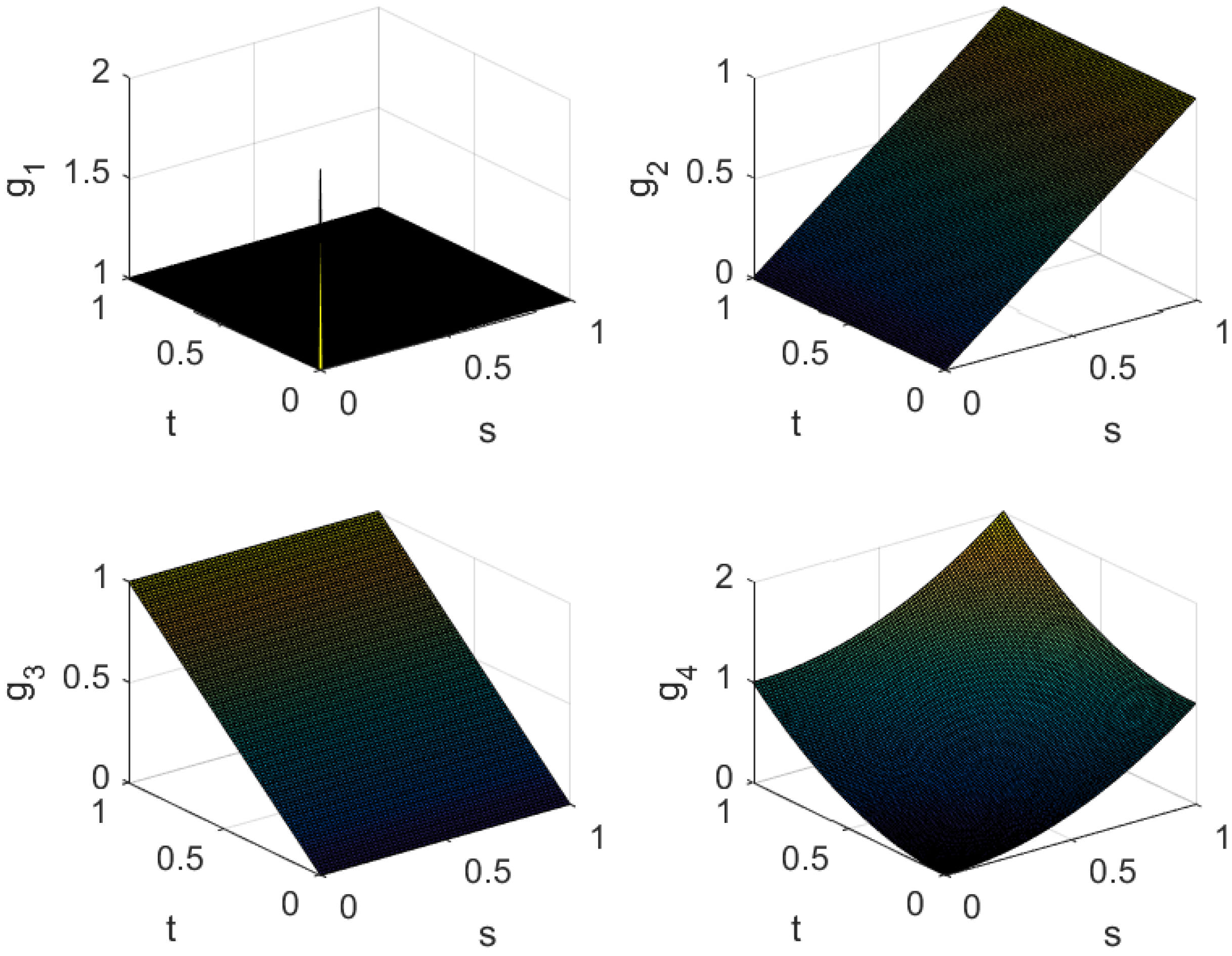
In light of the convergence properties of the sequence of positive linear operators $\left({\mathfrak{A}}_{i,j}\right)$, as established in Theorem 4 for the algebraic test functions 1, s, t, and $s^2+t^2$, we provide Figure 5, generated using MATLAB R2016b.

Figure 5. Convergence behavior of positive linear operators.

The convergence behavior of $\left({\mathfrak{A}}_{i,j}\right)$, as illustrated in Figure 5, yields the following key observations:

• Case of $\mathfrak{A}\mathit{i},\mathit{j}(\mathbf{1};\mathit{s},\mathit{t})$: The plot demonstrates that the operator preserves the constant function 1 under the action of the sequence $\left\{{\mathfrak{A}}_{\mathit{i},\mathit{j}}\right\}$. This confirms the positivity and normalization property, ensuring that the operator consistently approximates unity. The convergence to 1 across the domain ${[\mathbf{0},\mathbf{1}]}^{\mathbf{2}}$ highlights stability and validity in the approximation process.
• Case of ${\mathfrak{A}}_{\mathit{i},\mathit{j}}(\mathit{s};\mathit{s},\mathit{t})$: The graphical representation illustrates how the operator effectively approximates the identity function in the first variable. The convergence towards the function $\mathit{s}$ becomes evident as $\mathit{i},\mathit{j}\to \infty$, demonstrating the operator’s capability to preserve linearity in the $\mathit{s}$-direction. This validates one of the Korovkin-type test conditions for double sequences of operators.
• Case of ${\mathfrak{A}}_{\mathit{i},\mathit{j}}(\mathit{t};\mathit{s},\mathit{t})$: Similarly to the case of $\mathit{s}$, this figure shows the approximation behavior in the second variable $\mathit{t}$. The convergence toward $\mathit{t}$ indicates that the operators are capable of reproducing linear growth in the $\mathit{t}$-direction. Together with the $\mathit{s}$-direction, this ensures balanced approximation in both variables simultaneously.
• Case of ${\mathfrak{A}}_{\mathit{i},\mathit{j}}({\mathit{s}}^{\mathbf{2}}+{\mathit{t}}^{\mathbf{2}};\mathit{s},\mathit{t})$: This plot reflects the approximation of quadratic growth in both variables. The convergence towards ${\mathit{s}}^{\mathbf{2}}+{\mathit{t}}^{\mathbf{2}}$ indicates that the operators not only preserve constant and linear test functions but also accurately capture the curvature or second-order behavior of functions in two variables. This provides strong evidence of the robustness of the operators in approximating more complex functional behaviors.

The Figure 5 collectively establish that the operators $\left({\mathfrak{A}}_{i,j}\right)$ satisfy the Korovkin-type test conditions in the setting of functions of two variables for double sequences. Their convergence patterns confirm that these operators are reliable tools in approximation theory, ensuring deferred weighted statistically gauge (${\mathrm{stat}}_{\mathrm{DWG}}$) summability while simultaneously distinguishing themselves from the stricter ${\mathrm{DWG}}_{\mathrm{stat}}$ integrability criterion.

5. Conclusions

In this bottommost section of our study, we reaffirm the efficacy and potential impact of Theorems 3 and 4 in the context of double sequences for functions of two variables. The established results not only extend the classical Korovkin-type approximation framework to a richer setting but also demonstrate the nuanced distinction between deferred weighted statistically gauged (${\mathrm{DWG}}_{\mathrm{stat}}$) integrability and statistically deferred weighted gauged (${\mathrm{stat}}_{\mathrm{DWG}}$) summability. Through the construction of concrete examples and the graphical illustrations based on positive linear operators, it has been shown that while the two concepts are closely related, they exhibit subtle yet significant differences in approximation behavior.

The analysis for test functions 1, s, t, and $s^2+t^2$ has further validated the applicability of the developed operators, thereby ensuring that these theorems serve as a powerful tool in handling approximation problems in two-dimensional settings. This advancement provides a solid foundation for further explorations in approximation theory, particularly in the study of multivariate operators, sequence spaces, and their applications to diverse areas of applied mathematics. The results thus underscore not only the theoretical depth of the present study but also its potential to inspire new developments in the field.

Remark 1.

Consider the double sequence of functions ${\left(g_{i,j}\right)}_{i,j\in \mathbb{N}}$ as described in Example 4. Assume that ${\left(g_{i,j}\right)}_{i,j\in \mathbb{N}}$ is ${\mathrm{stat}}_{\mathrm{DWG}}$ summable, so that

$$\begin{array}{c}\hfill {\mathrm{stat}}_{\mathrm{DWG}}\underset{i,j\to \infty }{lim}\mathcal{G}(g_{i,j};\dot{\mathcal{P}})=0\mathrm{on}[0,1]\times [0,1].\end{array}$$

Then, we obtain

$$\begin{array}{c}\hfill {\mathrm{stat}}_{\mathrm{DWG}}\underset{i,j\to \infty }{lim}{\parallel {\mathfrak{A}}_{i,j}(g_{\upsilon };s,t)-g_{\upsilon }(s,t)\parallel }_{{[0,1]}^2}=0,(\upsilon =0,1,2,3).\end{array}$$

(21)

Therefore, by Theorem 4, it follows that

$$\begin{array}{c}\hfill {\mathrm{stat}}_{\mathrm{DWG}}\underset{i,j\to \infty }{lim}{\parallel {\mathfrak{A}}_{i,j}(g;s,t)-g(s,t)\parallel }_{{[0,1]}^2}=0,\end{array}$$

(22)

where the test functions are given by

$$\begin{array}{c}\hfill g_0(s,t)=1,g_1(s,t)=s,g_2(s,t)=t,g_3(s,t)=s^2+t^2.\end{array}$$

In this framework, the double sequence of functions $\left(g_{i,j}\right)$ satisfies the condition of statistical deferred weighted gauge summability ($\mathrm{stat}\mathrm{DWG}$). However, it does not fulfill the requirements for gauge integrability or $\mathrm{DWG}\mathrm{stat}$ integrability, as illustrated in Example 4. This distinction underscores the relevance of our Korovkin-type Theorem 4, which applies directly to the class of operators defined in (16). Furthermore, it highlights an important fact that statistical deferred weighted summability holds for these operators, whereas the corresponding notions of gauge integrability, both in the classical and weighted statistical sense, fail to coincide in this setting. As a result, Theorem 4 stands as a meaningful and substantial generalization, extending not only Theorem 3 but also enriching the classical Korovkin-type theorem [28], thereby broadening the scope of approximation processes in two variables.

Remark 2.

Motivated by the extensive survey and expository review presented by Srivastava [37], it is worth highlighting that the present line of investigation on approximation of functions of two variables via double sequences can naturally be broadened to incorporate the framework of q-calculus. Reformulating the operators studied in this paper within the realm of q-analysis would not only enhance their structural richness but also provide a wider platform for studying approximation processes in two dimensions.

In addition, a further refinement can be obtained by considering a $(p,q)$-extension of the proposed results. However, such an extension generally requires only minor adjustments, since the role of the parameter p tends to be auxiliary; the q-analog itself already embodies the essential aspect of the generalization. For a more detailed exposition of these ideas, including theoretical insights and practical illustrations, we refer the reader to Srivastava’s comprehensive work (see [37], p. 340).

References

1. Bartle, R.G. A Modern Theory of Integration; American Mathematical Society: Providence, RI, USA, 2000; Volume 32. [Google Scholar]
2. Fast, H. Sur la convergence statistique. Colloq. Math. 1951, 2, 241–244. [Google Scholar] [CrossRef]
3. Steinhaus, H. Sur la convergence ordinaire et la convergence asymptotique. Colloq. Math. 1951, 2, 73–74. [Google Scholar]
4. Baliarsingh, P. On statistical deferred A-convergence of uncertain sequences. Int. J. Uncertain. Fuzziness Knowl.-Based Syst. 2021, 29, 499–515. [Google Scholar] [CrossRef]
5. Belen, C.; Mohiuddine, S.A. Generalized statistical convergence and application. Appl. Math. Comput. 2013, 219, 9821–9826. [Google Scholar] [CrossRef]
6. Kadak, U. On weighted statistical convergence based on (p,q)-integers and related approximation theorems for functions of two variables. J. Math. Anal. Appl. 2016, 443, 752–764. [Google Scholar] [CrossRef]
7. Kadak, U.; Baliarsingh, P. On certain Euler difference sequence spaces of fractional order and related dual properties. J. Nonlinear Sci. Appl. 2015, 8, 997–1004. [Google Scholar] [CrossRef]
8. Kadak, U.; Mohiuddine, S.A. Generalized statistically almost convergence based on the difference operator which includes the (p,q)-gamma function and related approximation theorems. Results Math. 2018, 73, 9. [Google Scholar] [CrossRef]
9. Mohiuddine, S.A. Statistical weighted A-summability with application to Korovkin’s type approximation theorem. J. Inequal. Appl. 2016, 2016, 101. [Google Scholar] [CrossRef]
10. Mohiuddine, S.A.; Alamri, B.A. Generalization of equi-statistical convergence via weighted lacunary sequence with associated Korovkin and Voronovskaya type approximation theorems. Rev. Real Acad. Cienc. Exactas Fís. Nat. Ser. A Mat. (RACSAM) 2019, 113, 1955–1973. [Google Scholar] [CrossRef]
11. Mohiuddine, S.A.; Asiri, A.; Hazarika, B. Weighted statistical convergence through difference operator of sequences of fuzzy numbers with application to fuzzy approximation theorems. Int. J. Gen. Syst. 2019, 48, 492–506. [Google Scholar] [CrossRef]
12. Mohiuddine, S.A.; Hazarika, B.; Alghamdi, M.A. Ideal relatively uniform convergence with Korovkin and Voronovskaya types approximation theorems. Filomat 2019, 33, 4549–4560. [Google Scholar] [CrossRef]
13. Srivastava, H.M.; Jena, B.B.; Paikray, S.K. Statistical Riemann and Lebesgue integrable sequence of functions with Korovkin-type approximation theorems. Axioms 2021, 10, 229. [Google Scholar] [CrossRef]
14. Srivastava, H.M.; Jena, B.B.; Paikray, S.K. Some Korovkin-type approximation theorems associated with a certain deferred weighted statistical Riemann–integrable sequence of functions. Axioms 2022, 11, 128. [Google Scholar] [CrossRef]
15. Jena, B.B.; Paikray, S.K. A new approach to statistical Riemann-Stieltjes integrals. Miskolc Math. Notes 2023, 24, 789–803. [Google Scholar] [CrossRef]
16. Jena, B.B.; Paikray, S.K.; Dutta, H. Statistically Riemann integrable and summable sequence of functions via deferred Cesàro mean. Bull. Iran. Math. Soc. 2022, 48, 1293–1309. [Google Scholar] [CrossRef]
17. Parida, P.; Paikray, S.K.; Jena, B.B. Statistical Deferred Weighted Riemann Summability and Fuzzy Approximation Theorems. Sahand Commun. Math. Anal. 2023, 21, 327–345. [Google Scholar]
18. Acar, T.; Mohiuddine, S.A. Statistical (C,1)(E,1) summability and Korovkin’s theorem. Filomat 2016, 30, 387–393. [Google Scholar] [CrossRef]
19. Braha, N.L. Some weighted equi-statistical convergence and Korovkin type-theorem. Results Math. 2016, 70, 433–446. [Google Scholar] [CrossRef]
20. Edely, O.H.H.; Mohiuddine, S.A.; Noman, A.K. Korovkin type approximation theorems obtained through generalized statistical convergence. Appl. Math. Lett. 2010, 23, 1382–1387. [Google Scholar] [CrossRef]
21. Karakaya, V.; Chishti, T.A. Weighted statistical convergence. Iran. J. Sci. Technol. Trans. A Sci. 2009, 33, 219–223. [Google Scholar]
22. Mohiuddine, S.A. An application of almost convergence in approximation theorems. Appl. Math. Lett. 2011, 24, 1856–1860. [Google Scholar] [CrossRef]
23. Mohiuddine, S.A.; Alotaibi, A.; Mursaleen, M. Statistical summability (C,1) and a Korovkin-type approximation theorem. J. Inequal. Appl. 2012, 2012, 172. [Google Scholar] [CrossRef]
24. Mursaleen, M.; Belen, C. On statistical lacunary summability of double sequences. Filomat 2014, 28, 231–239. [Google Scholar] [CrossRef]
25. Mursaleen, M.; Karakaya, V.; Ertürk, M.; Gürsoy, F. Weighted statistical convergence and its application to Korovkin-type approximation theorem. Appl. Math. Comput. 2012, 218, 9132–9137. [Google Scholar] [CrossRef]
26. Saini, K.; Raj, K. Applications of statistical convergence in complex uncertain sequences via deferred Riesz mean. Int. J. Uncertain. Fuzziness Knowl.-Based Syst. 2021, 29, 337–351. [Google Scholar] [CrossRef]
27. Srivastava, H.M.; Mursaleen, M.; Khan, A. Generalized equi-statistical convergence of positive linear operators and associated approximation theorems. Math. Comput. Model. 2012, 55, 2040–2051. [Google Scholar] [CrossRef]
28. Korovkin, P.P. Convergence of linear positive operators in the spaces of continuous functions. Dokl. Akad. Nauk. SSSR (New Ser.) 1953, 90, 961–964. (In Russian) [Google Scholar]
29. Jena, B.B.; Paikray, S.K.; Mursaleen, M. Statistical gauge integrable functions and Korovkin-type approximation theorems. Bull. Iran. Math. Soc. 2025, 51, 47. [Google Scholar] [CrossRef]
30. Mishra, L.N.; Patro, M.; Paikray, S.K.; Jena, B.B. A certain class of statistical deferred weighted A-summability based on (p,q)-integers and associated approximation theorems. Appl. Math. 2019, 14, 716–740. [Google Scholar]
31. Rao, N.; Farid, M.; Raiz, M. On the approximations and symmetric properties of Frobenius-Euler-Şimşek polynomials connecting Szász operators. Symmetry 2025, 17, 648. [Google Scholar] [CrossRef]
32. Satapathy, A.; Jena, B.B.; Paikray, S.K. Korovkin-Type Approximation theorems for positive linear operators via statistical martingale sequences. Bol. Soc. Paran. Mat. 2025, 43, 1–12. [Google Scholar] [CrossRef]
33. Srivastava, H.M.; Jena, B.B.; Paikray, S.K. A new class of Korovkin-type theorems on double sequences. Iran. J. Sci. 2025, 49, 1103–1114. [Google Scholar] [CrossRef]
34. Srivastava, H.M.; Jena, B.B.; Paikray, S.K.; Misra, U.K. Korovkin-type theorems for positive linear operators based on the statistical derivative of deferred Cesàro summability. Algorithms 2025, 18, 218. [Google Scholar] [CrossRef]
35. Yildiz, S. Korovkin type approximation via statistical e-convergence on two dimensional weighted spaces. Math. Slovaca 2021, 71, 1167–1178. [Google Scholar] [CrossRef]
36. Altın, A.; Doǧru, O.; Taşdelen, F. The generalization of Meyer-König and Zeller operators by generating functions. J. Math. Anal. Appl. 2005, 312, 181–194. [Google Scholar] [CrossRef]
37. Srivastava, H.M. Operators of basic (or q-) calculus and fractional q-calculus and their applications in geometric function theory of complex analysis. Iran. J. Sci. Technol. Trans. A Sci. 2020, 44, 327–344. [Google Scholar] [CrossRef]
Disclaimer/Publisher’s Note: The statements, opinions and data contained in all publications are solely those of the individual author(s) and contributor(s) and not of MDPI and/or the editor(s). MDPI and/or the editor(s) disclaim responsibility for any injury to people or property resulting from any ideas, methods, instructions or products referred to in the content.
Article Metrics
Citations
Article Access Statistics
Multiple requests from the same IP address are counted as one view.