Estimating Smoothness and Optimal Bandwidth for Probability Density Functions

Abstract

The properties of non-parametric kernel estimators for probability density function from two special classes are investigated. Each class is parametrized with distribution smoothness parameter. One of the classes was introduced by Rosenblatt, another one is introduced in this paper. For the case of the known smoothness parameter, the rates of mean square convergence of optimal (on the bandwidth) density estimators are found. For the case of unknown smoothness parameter, the estimation procedure of the parameter is developed and almost surely convergency is proved. The convergence rates in the almost sure sense of these estimators are obtained. Adaptive estimators of densities from the given class on the basis of the constructed smoothness parameter estimators are presented. It is shown in examples how parameters of the adaptive density estimation procedures can be chosen. Non-asymptotic and asymptotic properties of these estimators are investigated. Specifically, the upper bounds for the mean square error of the adaptive density estimators for a fixed sample size are found and their strong consistency is proved. The convergence of these estimators in the almost sure sense is established. Simulation results illustrate the realization of the asymptotic behavior when the sample size grows large.

1. Introduction

Let $X_1,\dots ,X_n$ be independent identically distributed random variables (i.i.d. r.v.’s) having a probability density function f. In the typical non-parametric set-up, nothing is assumed about f except that it possesses a certain degree of smoothness, e.g., that it has r continuous derivatives.

Estimating f via kernel smoothing is a sixty year old problem; M. Rosenblatt who was one of its originators discusses the subject’s history and evolution in the monograph [1]. For some point x, the kernel smoothed estimator of $f(x)$ is defined by

$$f_{n,h}(x)=\frac{1}{n}\sum _{j=1}^n\frac{1}{h}K\left(\frac{x-X_j}{h}\right)$$

(1)

where the kernel $K(·)$ is a bounded function satisfying $\int K(x)dx=1$ and $\int K^2(x)dx<\infty$, and the positive bandwidth parameter h is a decreasing function of the sample size n.

If $K(·)$ has finite moments up to q-th order, and moments of order up to $q-1$ equal to zero, then q is called the ‘order’ of the kernel $K(·)$. Since the unknown function f is assumed to have r continuous derivatives, it typically follows that

$$Var(f_{n,h}(x))=\frac{C_{f,K}(x)}{hn}+o\left(\frac{1}{hn}\right),$$

and

$$Bias(f_{n,h}(x))=c_{f,K}(x)h^k+o(h^k),$$

where $k=min(q,r)$, and $C_{f,K}(x),c_{f,K}(x)$ are bounded functions depending on $K(·)$ as well as f and its derivatives, cf. [1] p. 8.

The idea of choosing a kernel of order q bigger (or equal) than r in order to ensure the $Bias(f_{n,h}(x))$ to be $O(h^r)$ dates back to the early 1960s in work of [2,3]; recent references on higher-order kernels include the following: [4,5,6,7,8,9,10]. Note that since r is typically unknown and can be arbitrarily large, it is possible to use kernels of infinite order that achieve the minimal bias condition $Bias(f_{n,h}(x))=O(h^r)$ for any r; Ref. [11] gives many properties of kernels of infinite order. In this paper we will employ a particularly useful class of infinite order kernels namely the flat-top family; see [12] for a general definition.

It is a well-known fact that optimal bandwidth selection is perhaps the most crucial issue in such non-parametric smoothing problems; see [13], as well as the book [14]. The goal typically is minimization of the large-sample mean squared error (MSE) of $f_{n,h}(x)$. However, to perform this minimization, the practitioner needs to know the degree of smoothness r, as well as the constants $C_{f,K}(x)$ and $c_{f,K}(x)$. Using an infinite order kernel and focusing just on optimizing the order of magnitude of the large-sample MSE, it is apparent that the optimal bandwidth h must be asymptotically of order $n^{-1/(2r+1)}$; this yields a large-sample MSE of order $n^{-2r/(2r+1)}$.

A generalization of the above scenario is possible using a degree of smoothness r that has another sense, and that is not necessarily an integer. Let $\left[r\right]$ denote the integer part of r, and define $\gamma =r-\left[r\right]$; then, one may assume that f has $\left[r\right]$ continuous derivatives, and that the $\left[r\right]$th derivative satisfies a Lipschitz condition of order $\gamma$. Interestingly, even in this case where f is assumed to belong to the Hölder class of degree r (the derivative of the density function of the order r satisfies the Lipschitz condition) the MSE–optimal bandwidth h is still of order $n^{-1/(2r+1)}$ and again yields a large-sample MSE of the order $n^{-2r/(2r+1)}$ (see, e.g., [15,16,17,18] among others).

The problem of course is that, as previously mentioned, the underlying degree of smoothness r is typically unknown. In Section 4 of the paper at hand, we develop an estimator $r_n$ of r and prove its strong consistency; this is perhaps the first such result in the literature. In order to construct our estimator $r_n$, we operate under a class of functions that is slightly more general than the aforementioned Hölder class; this class of functions is formally defined in Section 2 via Equation (3) or (4).

Under such a condition on the tails of the characteristic function we are able to show in Section 3 that the optimized MSE of ${\widehat{f}}_n(x)$ is again of order $n^{-2r/(2r+1)}$ for possibly non-integer $r;$ this is true, for example, when the characteristic function $\varphi (s)$ has tails of order $O(1/|s{|}^{r+1}),$ see Example 2.

Furthermore, in Section 5 we develop an adaptive estimator ${\widehat{f}}_n(x)$ that achieves the optimal MSE rate of $n^{-2r/(2r+1)}$ within a logarithmic factor despite the fact that r is unknown, see Examples after Theorem 3. Similar effect arises in the adaptive estimation problem of the densities from the Hölder class; see [18,19,20]. It should pointed that problems of asymptotic adaptive optimal density estimations from another classes have also been considered in the literature; see, e.g., [14,21,22,23].

The construction of ${\widehat{f}}_n(x)$ is rather technical; it uses the new estimator $r_n$, and it is inspired from the construction of sequential estimates although we are in a fixed n, non-sequential setting. As the major theoretical result of our paper, we are able to prove a non-asymptotic upper bound for the MSE of ${\widehat{f}}_n(x)$ that satisfies the above mentioned optimal rate. Section 6 contains some simulation results showing the performance of the new estimator ${\widehat{f}}_n(x)$ in practice. All proofs are deferred to Section 7, while Section 8 contains our conclusions and suggestions for future work.

2. Problem Set-Up and Basic Assumptions

Let $X_1,\dots ,X_n$ be i.i.d. having a probability density function f. Denote ${\displaystyle \varphi (s)=\int {\mathrm{e}}^{isx}f(x)dx}$ the characteristic function of f and the sample characteristic function ${\displaystyle {\varphi }_n(s)=\frac{1}{n}\sum _{k=1}^n{\mathrm{e}}^{is{X}_k}.}$ For some finite $r>0$, define two families ${\mathcal{F}}_r^{+}$ and ${\mathcal{F}}_r$ of bounded, i.e.,

$${\displaystyle \exists 0<\overline{f}<\infty :\underset{y\in {\mathcal{R}}^1}{sup}f(y)\le \overline{f},}$$

(2)

and continuous functions f satisfying one of the following conditions, respectively:

$$\int {|s|}^r|\varphi (s)|ds<\infty ,\int {|s|}^{r+\epsilon }|\varphi (s)|ds=\infty ,\mathrm{for}\mathrm{all}\epsilon >0,$$

(3)

$$\int {|s|}^{r-\epsilon }|\varphi (s)|ds<\infty ,\int {|s|}^r|\varphi (s)|ds=\infty ,\mathrm{for}\mathrm{all}0<\epsilon <r.$$

(4)

In other words, ${\mathcal{F}}_r^{+}$ is the family of functions (introduced by M. Rosenblatt) satisfying (2) and (3), while ${\mathcal{F}}_r$ is the family of functions (introduced in this paper) satisfying (2) and (4). It should be noted that the new class ${\mathcal{F}}_r$ is a little bit more wide that the classical class ${\mathcal{F}}_r^{+}$.

In addition, define the family ${\mathcal{F}}_{r,m}^{+}$ (respectively, ${\mathcal{F}}_{r,m}$) as the family of functions f that belong to ${\mathcal{F}}_r^{+}$ (respectively, ${\mathcal{F}}_r$) but with f being such that its characteristic function $|\varphi (s)|$ has monotonously decreasing tails.

Consider the class $\mathrm{\Xi }$ of non-parametric kernel smoothed estimators $f_{n,h}(x)$ of $f(x)$ as given in Equation (1). Note that we can alternatively express $f_{n,h}(x)$ in terms of the Fourier transform of kernel $K(·)$, i.e.,

$$f_{n,h}(x)=\frac{1}{n}\sum _{j=1}^n\frac{1}{h}K\left(\frac{x-X_j}{h}\right)=\frac{1}{2\pi }\int \lambda (s,h){\varphi }_n(s){\mathrm{e}}^{-isx}ds$$

(5)

where

$$\lambda (s,h)=\int K\left(\frac{x}{h}\right)e^{isx}dx.$$

In this paper, we will employ the family of flat-top infinite order kernels, i.e., we will let the function $\lambda (s,h)$ be of the form

$${\displaystyle {\lambda }_c(s,h)=\left\{\begin{array}{c}1\mathrm{if}\left|s\right|\le 1/h,\hfill \\ g(s,h)\mathrm{if}1/h<\left|s\right|\le c/h,\hfill \\ 0\mathrm{if}\left|s\right|\ge c/h,\hfill \end{array}\right.}$$

where c is a fixed number in $[1,\infty )$ chosen by the practitioner, and $g(s,h)$ is some properly chosen continuous, real-valued function satisfying $g(s,h)=g(-s,h),$ $g(s,1)=g(s/h,h),$ and $|g(s,h)|\le 1,$ for any $s,$ with $g(1/h,h)=1,$ and $g(c/h,h)=0$; see [12,24,25,26] for more details on the above flat-top family of kernels.

Define $g_h^{\prime }(s,h)$ the partial derivative of the function $g(s,h)$ with respect to the bandwidth $h.$ We will also assume that for some $c_0>0$

$${\displaystyle \overline{\underset{h\to 0}{lim}}\underset{1/h<\left|s\right|<c/h}{sup}|g_h^{\prime }(s,h)|/|s|<c_0.}$$

(6)

Denote for every $0\le \gamma <r$ the functions

$${\delta }_{\gamma }(h)=\underset{1/h<\left|s\right|<c/h}{\int }{\left|s\right|}^{r-\gamma }\left|\varphi (s)\right|ds,\mathrm{when}h>0,\mathrm{and}{\delta }_{\gamma }(0)=0.$$

From (3) and (5) it follows that ${\delta }_{\gamma }(h)=o(1)$ as $h\to 0$ for $f\in {\mathcal{F}}_r^{+}$ and $\gamma =0,$ as well as for $f\in {\mathcal{F}}_r$ and $0<\gamma <r.$ In other cases ${\delta }_{\gamma }(h)=\infty .$

Define the following classes ${\overline{\mathcal{F}}}_r={\mathcal{F}}_r^{+}\cup {\mathcal{F}}_r$ and ${\overline{\mathcal{F}}}_{r,m}={\mathcal{F}}_{r,m}^{+}\cup {\mathcal{F}}_{r,m}.$

The main aim of the paper is the estimation of the parameter r of these classes and adaptive estimation of densities from the class ${\overline{\mathcal{F}}}_r$ with the unknown parameter $r.$

3. Asymptotic Mean Square Optimal Estimation

The mean square error (MSE) $u_f^2(f_{n,h})=E_f{(f_{n,h}(x)-f(x))}^2$ of the estimators $f_{n,h}(x)\in \mathrm{\Xi },$$f\in {\overline{\mathcal{F}}}_r$ has the following form:

$${\displaystyle u_f^2(f_{n,h})=U_f^2(h,c)-\frac{1}{n}{\left(\int K(v)f(x-hv)dv\right)}^2,}$$

(7)

where $U_f^2(h,c)$ is the principal term of the MSE,

$$U_f^2(h,c)=\frac{L_{1}f(x)}{nh}+{\left[\frac{1}{2\pi }\underset{1/h<\left|s\right|<c/h}{\int }(1-g(s,h))\varphi (s){\mathrm{e}}^{-isx}ds\right]}^2,$$

${\displaystyle L_1=\int K^2(v)dv.}$ Thus, in particular, ${\displaystyle \underset{f\in {\overline{\mathcal{F}}}_r}{sup}\left|\int K(v)f(x-hv)dv\right|<\infty .}$

To minimize the principal term $U_f^2(h,c)$ by h we set its first derivative with respect to ${\displaystyle h}$ to zero which gives the following equality for the optimal (in the mean square sense) value $h^0=h^0(n):$

$$\begin{gathered} {\displaystyle \underset{1/h^0<\left|s\right|<c/h^0}{\int }(g(s,h^0)-1)\varphi (s){\mathrm{e}}^{-isx}ds·\{c\varphi (c/h^0){\mathrm{e}}^{-\frac{icx}{h^0}}+c\varphi (-c/h^0){\mathrm{e}}^{\frac{icx}{h^0}}} \\ {\displaystyle +{(h^0)}^2\underset{1/h^0<\left|s\right|<c/h^0}{\int }{g}_h^{\prime }(s,h^0)\varphi (s){\mathrm{e}}^{-isx}ds\}=\frac{2{\pi }^2{L}_{1}f(x)}{n}.} \end{gathered}$$

(8)

From the definition of the class of kernels for cases ${\delta }_{\gamma }(h)<\infty$ we have

$$\left|\underset{ 1/h<\left|s\right|<c/h}{\int }(g(s,h)-1)\varphi (s){\mathrm{e}}^{-isx}ds\right|\le 2h^{r-\gamma }{\delta }_{\gamma }(h)$$

and for h small enough, according to (6)

$$\left|\underset{ 1/h<\left|s\right|<c/h}{\int }{g}_h^{\prime }(s,h)\varphi (s){\mathrm{e}}^{-isx}ds\right|\le c_0{h}^{r-1-\gamma }{\delta }_{\gamma }(h).$$

Then, by the definition of the class ${\overline{\mathcal{F}}}_{r,m},$ as h small enough, denoting ${\displaystyle c_1(\gamma )=\frac{r+1-\gamma }{2(c^{r+1-\gamma }-1)},}$ we have

$${\delta }_{\gamma }(h)\ge \underset{1/h}{\overset{c/h}{\int }}{\left|s\right|}^{r-\gamma }ds·[\underset{1/h<s<c/h}{inf}\left|\varphi (s)\right|+\underset{1/h<s<c/h}{inf}\left|\varphi (-s)\right|]$$

$$\ge {(c_1(\gamma ))}^{-1}{h}^{-(r+1-\gamma )}\left[\right|\varphi (c/h)|+\left|\varphi (-c/h)\right|].$$

Thus, for $h<<1,$

$$\left|\varphi (c/h)\right|+\left|\varphi (-c/h)\right|\le c_1(\gamma )h^{r+1-\gamma }{\delta }_{\gamma }(h)$$

and from (8) it follows

$${\displaystyle {(h^0)}^{2r+1-2\gamma }{\delta }_{\gamma }^2(h^0)\ge \frac{{\pi }^2{L}_{1}f(x)}{(c_0+c_1(\gamma ))n}.}$$

Define the number $h_1^0=h_1^0(n)$ from the equality

$${\displaystyle {(h_1^0)}^{2r+1-2\gamma }{\delta }_{\gamma }^2(h_1^0)=\frac{{\pi }^2{L}_{1}f(x)}{(c_0+c_1(\gamma ))n}.}$$

(9)

It is obvious, that $0<h_1^0\le h^0$ and ${(h_1^0)}^{2r+1-2\gamma }{\delta }_{\gamma }^2(h_1^0)\le {(h^0)}^{2r+1-2\gamma }{\delta }_{\gamma }^2(h^0).$

Then, from (7) and (9), for every $f\in {\overline{\mathcal{F}}}_{r,m}$ and $f_n^0=f_{n,h^0}$ as $n\to \infty ,$ we have

$$\begin{gathered} {\displaystyle u_f^2(f_n^0)\le u_f^2(f_{n,h_1^0})\le \frac{L_{1}f(x)}{n{h}_1^0}+\frac{1}{{\pi }^2}{(h_1^0)}^{2r-2\gamma }{\delta }_{\gamma }^2(h_1^0)} \\ {\displaystyle =C_{\gamma }·\frac{{\delta }_{\gamma }^{\frac{2}{2r+1-2\gamma }}(h_1^0)}{n^{\frac{2r-2\gamma }{2r+1-2\gamma }}},} \end{gathered}$$

(10)

where

$$C_{\gamma }=L_1^{\frac{2r-2\gamma }{2r+1-2\gamma }}(x)\left(1+\frac{{\pi }^2}{c_0+c_1(\gamma )}\right){\left(\frac{c_0+c_1(\gamma )}{{\pi }^2}\right)}^{\frac{1}{2r+1-2\gamma }}.$$

In such a way we have proved the following theorem, which gives the rates of convergence of the random quantities $f_n^0(x)$ and $f_{n,h_1^0}(x).$ We can loosely call $f_n^0(x)$ and $f_{n,h_1^0}(x)$ ‘estimators’ although it is clear that these functions can not be considered as estimators in the usual sense in view of the dependence of the bandwidths $h^0$ and $h_1^0$ on unknown parameters r and $f(x).$ Nevertheless, this theorem can be used for the construction of bona fide adaptive estimators with the optimal and suboptimal converges rates; see Examples 1 and 2, as well as Section 5.3 in what follows.

Theorem 1.

Let $f(x)>0.$ Then, for the asymptotically optimal (with respect to bandwidth h) in the MSE sense ‘estimator’ $f_n^0(x)$ of the function $f\in {\overline{\mathcal{F}}}_r$ and for the ‘estimator’ $f_{n,h_1^0}(x)$ of $f\in {\overline{\mathcal{F}}}_{r,m}$ the following limit relations, as $n\to \infty ,$ hold

$$\begin{array}{ccc}& & {\displaystyle 1^{\circ }.\underset{f\in {\overline{\mathcal{F}}}_r}{sup}\left|\underset{h}{inf}{u}_f^2(f_{n,h})-U_f^2(h^0,c)\right|=O\left(\frac{1}{n}\right);}\hfill \\ & & {\displaystyle 2^{\circ }.for everyf\in {\overline{\mathcal{F}}}_{r,m}with\gamma =0iff\in {\mathcal{F}}_{r,m}^{+}and every0<\gamma <riff\in {\mathcal{F}}_{r,m}}\hfill \\ & & u_f^2(f_n^0)\le u_f^2(f_{n,h_1^0})\le C_{\gamma }·\frac{{\delta }_{\gamma }^{\frac{2}{2r+1-2\gamma }}(h_1^0)}{n^{\frac{2r-2\gamma }{2r+1-2\gamma }}},n\ge 1.\hfill \end{array}$$

Remark 1.

The definition (9) of $h_1^0$ is essentially simpler than the definition (8) of the optimal bandwidth $h^0.$ From Theorem 1 it follows that the (slightly) suboptimal ‘estimator’ $f_{n,h_1^0}$ can be successfully used instead.

It should be noted that the parameter $\gamma$ is chosen by the practitioner here and that $\gamma =0\mathrm{if}f\in {\mathcal{F}}_{r,m}^{+}$ but $0<\gamma <r\mathrm{if}f\in {\mathcal{F}}_{r,m}$ in which case we want to choose $\gamma$ close to 0.

We shall write in the sequel $\phi (s)\approx \psi (s)$ as $s\to \infty$ instead of the limit relations

$$0<\underset{\overline{s\to \infty }}{lim}\frac{\phi (s)}{\psi (s)}\le \overline{\underset{s\to \infty }{lim}}\frac{\phi (s)}{\psi (s)}<\infty .$$

Example 1.

Consider an estimation problem of the function $f\in {\mathcal{F}}_{r,m}^{+},$ satisfying the following additional condition

$${\displaystyle \left|\varphi (s)\right|\approx \frac{1}{{\left|s\right|}^{r+1}{ln}^{1+\phi }\left|s\right|}as\left|s\right|\to \infty ,\phi >0,}$$

using the kernel estimator $(f_{n,h}(x))\in \mathrm{\Xi }.$

By making use of (9) and (10) we find the rate of convergence of the MSE $u_f^2(f_n^0)$ and $u_f^2(f_{n,h_1^0}).$ To this end we calculate

$${\delta }_0(h)=\underset{1/h<\left|s\right|<c/h}{\int }{\left|s\right|}^r\left|\varphi (s)\right|ds\approx \frac{1}{{(ln{h}^{-1})}^{\phi }}-\frac{1}{{(ln{h}^{-1}+lnc)}^{\phi }}\approx \frac{1}{{({ln}^2{h}^{-1})}^{1+\phi }}.$$

It is easy to verify that $f_n^0,f_{n,h_1^0}\in \mathrm{\Xi }.$ Thus, from (9), as $n\to \infty ,$

$$h_1^0\approx {(n{\gamma }_n)}^{-\frac{1}{2r+1}},$$

where ${\gamma }_n\approx {ln}^{-2(1+\phi )}n,n\to \infty$ is a solution of the equation

$${\gamma }_n{[lnn+ln{\gamma }_n]}^{2(1+\phi )}=1.$$

Therefore, as $n\to \infty ,$ we have

$${\displaystyle h_1^0\approx {\left(\frac{{ln}^{2(1+\phi )}n}{n}\right)}^{\frac{1}{2r+1}}and{u}_f^2(f_{n,h_1^0})=O{\left(\frac{1}{n^{2r}{ln}^{2(1+\phi )}n}\right)}^{\frac{1}{2r+1}}.}$$

Consider the piecewise linear flat-top kernel ${\lambda }_c^{LIN}(s,h),$ introduced by [25] (see [26] as well):

$${\displaystyle {\lambda }_c^{LIN}(s,h)=\frac{c}{c-1}{\left(1-\frac{h}{c}\left|s\right|\right)}^{+}-\frac{1}{c-1}{\left(1-h\left|s\right|\right)}^{+},}$$

where ${(x)}^{+}=max(x,0)$ is the positive part function.

Then, from (8) we obtain

$${\displaystyle {\{\varphi (c/h^0){\mathrm{e}}^{-\frac{icx}{h^0}}+\varphi (-c/h^0){\mathrm{e}}^{\frac{icx}{h^0}}\}}^2\approx \frac{1}{n}}$$

and, for n large enough

$${\displaystyle {|\varphi (c/h^0)|}^2+{\left|\varphi (-c/h^0)\right|}^2\ge \frac{C}{n}.}$$

Thus, similarly to $h_1^0,$ as $n\to \infty ,$ for $f\in {\mathcal{F}}_r$ we find

$${\displaystyle h^0\approx {\left(\frac{{ln}^{2(1+\phi )}n}{n}\right)}^{\frac{1}{2(r+1)}}}$$

and

$${\displaystyle u_f^2(f_n^0)=O{\left(\frac{1}{n^{2r+1}{ln}^{2(1+\phi )}n}\right)}^{\frac{1}{2(r+1)}}=o\left(u_f^2(f_{n,h_1^0})\right).}$$

Example 2.

Consider an estimation problem of the function $f\in {\mathcal{F}}_{r,m},$ satisfying the following additional condition:

$${\displaystyle \left|\varphi (s)\right|\approx \frac{1}{{\left|s\right|}^{r+1}}as\left|s\right|\to \infty ,}$$

using the kernel estimator $(f_{n,h}(x))\in \mathrm{\Xi }.$

Using (9) and (10) we will find the rate of convergence of the MSE $u_f^2(f_n^0)$ and $u_f^2(f_{n,h_1^0}).$ To this end, we calculate

$${\delta }_{\gamma }(h)=\underset{1/h<\left|s\right|<c/h}{\int }{\left|s\right|}^{r-\gamma }\left|\varphi (s)\right|ds\approx h^{\gamma }.$$

It is easy to verify that $f_n^0,f_{n,h_1^0}\in \mathrm{\Xi }.$ Thus, from (9), as $n\to \infty ,$

$$h_1^0\approx n^{-\frac{1}{2r+1}}.$$

Therefore, we have

$${\displaystyle u_f^2(f_{n,h_1^0})=O\left(\frac{1}{n^{\frac{2r}{2r+1}}}\right),n\to \infty .}$$

Similarly to Example 1 as $n\to \infty ,$ for $f\in {\mathcal{F}}_r$ we find

$${\displaystyle h^0\approx \frac{1}{n^{\frac{1}{2(r+1)}}}}$$

and

$${\displaystyle u_f^2(f_n^0)=O\left(\frac{1}{n^{\frac{2r+1}{2(r+1)}}}\right)=o\left(u_f^2(f_{n,h_1^0})\right).}$$

4. Estimation of the Degree of Smoothness r

Define the functions

$${\mathsf{\Phi }}_{\alpha }(A,B)=\underset{A<\left|s\right|<B}{\int }{\left|s\right|}^{\alpha }\left|\varphi (s)\right|ds,{\mathsf{\Phi }}_{\alpha }={\mathsf{\Phi }}_{\alpha }(0,\infty ),$$

$${\mathsf{\Phi }}_{n,\alpha }(A,B)=\underset{A<\left|s\right|<B}{\int }{\left|s\right|}^{\alpha }\left|{\varphi }_n(s)\right|ds,{\mathsf{\Phi }}_{n,\alpha }={\mathsf{\Phi }}_{n,\alpha }(0,\infty ).$$

Let ${({\delta }_n)}_{n\ge 1}$ and ${({\rho }_n)}_{n\ge 1}$ be two given sequences of positive numbers chosen by the practitioner such that ${\delta }_n\to 0$ and ${\rho }_n\to \infty$ as $n\to \infty .$ The sequence $({\delta }_n)$ represents the ‘grid’-size in our search of the correct exponent $r,$ while $({\rho }_n)$ represents an upper bound that limits this search.

Define the following sets of non-random sequences

$${\displaystyle {\mathcal{C}}_{+}=\{{(A_n,B_n,{\delta }_n)}_{n\ge 1}:A_n\to \infty ,0<A_n<B_n\to \infty ,{\delta }_n\to 0\mathrm{as}n\to \infty ;}$$

$$\mathrm{for} \mathrm{some}{m}_0\ge 2,\sum _{n\ge 1}\frac{B_n^{2m_0({\varrho }_n+1+{\delta }_n)}}{n^{m_0}}<\infty ;{\mathsf{\Phi }}_{r+\epsilon }(A_n,B_n)\to \infty ,\forall \epsilon >0\},$$

$${\displaystyle \mathcal{C}=\{{(A_n,B_n,{\delta }_n)}_{n\ge 1}:A_n\to \infty ,0<A_n<B_n\to \infty ,{\delta }_n\to 0\mathrm{as}n\to \infty ;}$$

$$\mathrm{for} \mathrm{some}{m}_0\ge 2,\sum _{n\ge 1}\frac{B_n^{2m_0({\varrho }_n+1+{\delta }_n)}}{n^{m_0}}<\infty ;{\mathsf{\Phi }}_r(A_n,B_n)\to \infty \}.$$

Remark 2.

Formally, the definition of sets ${\mathcal{C}}_{+},$$\mathcal{C}$ and, as follows of estimators $r_n^{+}$ and $r_n,$ as well of sets ${\mathcal{C}}_{+}^{*},$${\mathcal{C}}_{*}$ defined below depend on the unknown function ${\mathsf{\Phi }}_{\alpha }(A,B).$ At the same time, the set ${\mathcal{C}}_{+}$ (and, as follows, the estimator $r_n^{+}$ and the set ${\mathcal{C}}_{+}^{*})$ can be defined independently of ${\mathsf{\Phi }}_{\alpha }(A,B).$

Indeed, denote ${\alpha }_s={\left|s\right|}^{r+1}\left|\varphi (s)\right|$ and

– let $f\in {\mathcal{F}}_r^{+}.$

Then for every $\epsilon >0$

$$\underset{s\to \infty }{lim}{s}^{\epsilon /2}{\alpha }_s=\infty and\overline{\underset{s\to \infty }{lim}}{\alpha }_s·logs<\infty .$$

Thus $(A_n,B_n,{\delta }_n)\in {\mathcal{C}}_{+}$ for appropriate chosen $({\delta }_n)$ and $A_n=O(B_n^{1/2})$ because (consider for simplification the case $A_n>0)$

$$\begin{gathered} {\mathsf{\Phi }}_{r+\epsilon }(A_n,B_n)={\int }_{A_n}^{B_n}{\left|s\right|}^{r+\epsilon }\left|\varphi (s)\right|ds={\int }_{A_n}^{B_n}{s}^{\epsilon -1}{\alpha }_{s}ds={\int }_0^{B_n}{s}^{\epsilon -1}{\alpha }_{s}ds-{\int }_0^{A_n}{s}^{\epsilon -1}{\alpha }_{s}ds \\ \ge C_1{\int }_0^{B_n}{s}^{\epsilon /2-1}ds-C_2{\int }_0^{A_n}{s}^{\epsilon -1}{log}^{-1}sds\sim B_n^{\epsilon /2}-A_n^{\epsilon }{log}^{-1}{A}_n \\ +{\int }_0^{A_n}{s}^{\epsilon -1}{log}^{-2}sds\to \infty . \end{gathered}$$

According to the definition of the class ${\mathcal{F}}_r$ it is impossible to find elements of the set $\mathcal{C}$ independently of the function to be estimated without usage of an a priori information about $f.$ Consider one simple example.

– Let $f\in {\mathcal{F}}_r.$

Suppose, e.g., in addition that

$$\underset{\overline{s\to \infty }}{lim}logs·\frac{1}{s}{\int }_0^s{\left|u\right|}^{r+1}\left|\varphi (u)\right|du>0.$$

Then $(A_n,B_n,{\delta }_n)\in \mathcal{C}$ for appropriate chosen $({\delta }_n)$ and $A_n=o(B_n)$ because

$$\begin{gathered} {\mathsf{\Phi }}_r(A_n,B_n)={\int }_{A_n}^{B_n}{s}^r\left|\varphi (s)\right|ds={\int }_{A_n}^{B_n}{s}^{-1}d{\int }_0^s{\alpha }_{u}duds=\frac{1}{s}{\int }_0^s{\alpha }_{u}du{|}_{A_n}^{B_n} \\ +{\int }_{A_n}^{B_n}{s}^{-2}{\int }_0^s{\alpha }_{u}duds\ge C{\int }_{A_n}^{B_n}\frac{1}{slogs}ds\ge Cloglog{B}_n\to \infty . \end{gathered}$$

Another examples are in Example 3 (see also Remark 3 and Example 4).

For an arbitrary given $H>0$ chosen by the practitioner, define the estimators ${(r_n^{+})}_{n\ge 1}$ and ${(r_n)}_{n\ge 1}$ of the parameter r in (3) and (4) as follows

$${\displaystyle r_n^{+}=min[{\varrho }_n,({\delta }_n·inf\{k\ge 1:{\mathsf{\Phi }}_{n,(k+1){\delta }_n}(A_n,B_n)\ge H,(A_n,B_n,{\delta }_n)\in {\mathcal{C}}_{+}\})].}$$

(11)

$${\displaystyle r_n=min[{\varrho }_n,({\delta }_n·inf\{k\ge 1:{\mathsf{\Phi }}_{n,k{\delta }_n}(A_n,B_n)\ge H,(A_n,B_n,{\delta }_n)\in \mathcal{C}\})].}$$

(12)

Example 3.

For the functions $\varphi (·)$ from Examples 1 and 2, we can use the definitions (11) and (12) with the following choices:

$$B_n=lnn,{\varrho }_n=\rho \frac{lnn}{lnlnn},\rho \in (0,{(2m_0)}^{-1}),$$

arbitrary ${\delta }_n\to 0$ and $A_n=o(B_n),$ as $n\to \infty .$ Indeed, for $f\in {\mathcal{F}}_{r,m}^{+}$ and every $\epsilon >0$ (Example 1),

$${\displaystyle {\mathsf{\Phi }}_{r+\epsilon }(A_n,B_n)=\underset{A_n<\left|s\right|<B_n}{\int }{\left|s\right|}^{r+\epsilon }\left|\varphi (s)\right|ds\approx \frac{B_n^{\epsilon }}{{ln}^{\phi }{B}_n}-\frac{A_n^{\epsilon }}{{ln}^{\phi }{A}_n}\approx \frac{{ln}^{\epsilon }n}{{ln}^{\phi }lnn}\to \infty }$$

and for $f\in {\mathcal{F}}_{r,m}$ (Example 2),

$${\displaystyle {\mathsf{\Phi }}_r(A_n,B_n)=\underset{A_n<\left|s\right|<B_n}{\int }{\left|s\right|}^r\left|\varphi (s)\right|ds\approx ln\frac{B_n}{A_n}\to \infty }$$

and, as follows, the classes ${\mathcal{C}}_{+}$ and $\mathcal{C}$ are not empty.

Define

$$J_{n,\alpha }=\underset{A_n<\left|s\right|<B_n}{\int }{\left|s\right|}^{\alpha }|{\varphi }_n(s)-\varphi (s)|ds,\alpha >0,n\ge 1.$$

Lemma 1.

Let ${\displaystyle (A_n,B_n,{\delta }_n)\in {\mathcal{C}}_{+}\cup \mathcal{C}.}$ Then, for every $\alpha >0,m\ge 1$ and $n\ge 1$ there exist positive numbers $C_{\alpha ,m}$ such that

$$\underset{f\in {\overline{\mathcal{F}}}_r}{sup}{E}_f{J}_{n,\alpha }^{2m}\le C_{\alpha ,m}\frac{B_n^{2m(\alpha +1)}}{n^m}$$

(13)

and for every $f\in {\overline{\mathcal{F}}}_r$

$$J_{n,{\varrho }_n+{\delta }_n}=o(1)P_f-a.s.$$

Define the sets ${\mathcal{C}}_{+}^{*}$ and ${\mathcal{C}}^{*}$ of non-random sequences ${(A_n,B_n,{\delta }_n)}_{n\ge 1}$

$${\mathcal{C}}_{+}^{*}=\{(A_n,B_n,{\delta }_n)\in {\mathcal{C}}_{+}:\underset{n\to \infty }{lim}{\mathsf{\Phi }}_{r+{\delta }_n}(A_n,B_n)=\infty \},$$

$${\mathcal{C}}_{*}=\{(A_n,B_n,{\delta }_n)\in \mathcal{C}:\underset{n\to \infty }{lim}{\mathsf{\Phi }}_{r-{\delta }_n}(A_n,B_n)=0\}.$$

Remark 3.

It can be directly verified that under the conditions of Remark 2 the sequences $(A_n,B_n,{\delta }_n)\in {\mathcal{C}}_{+}^{*}$ if $A_n=O(B_n^{1/2})$ and ${\delta }_n^{-1}=o(log{B}_n),$ as well as $(A_n,B_n,{\delta }_n)\in {\mathcal{C}}_{*}$ if $A_n=o(B_n)$ and

$${\delta }_n=o\left(\frac{logloglog{B}_n}{log{B}_n}\right).$$

Moreover, under the conditions of Example 3.1, $(A_n,B_n,{\delta }_n)\in {\mathcal{C}}_{+}^{*}$ if we put

$${\displaystyle {\delta }_n=\delta ·\frac{lnlnln(n+1)}{lnln(n+1)},\delta >\phi .}$$

Example 4.

Consider the functions $\varphi (·)$ from Examples 1, 2 and suppose, that the smooth parameter $r\le R$ for some known number $R.$ Then the sequences $(A_n,B_n,{\delta }_n)\in {\mathcal{C}}_{+}^{*}\cup {\mathcal{C}}_{*}$ if we put

$${\displaystyle B_n=n^b,0<b<\frac{m_0-1}{4(R+1)},A_n=o(B_n),{\varrho }_n=R,}$$

$${\displaystyle {\delta }_n=\delta ·\frac{lnln(n+1)}{ln(n+1)},\delta b>\phi .}$$

Theorem 2.

The estimators $r_n^{+}$ and $r_n,$ defined in (11) and (12), respectively, with ${\rho }_n\to \infty$ have the following properties

$1^{\circ }$

(a) if $f\in {\mathcal{F}}_r^{+}$ and ${\displaystyle (A_n,B_n,{\delta }_n)\in {\mathcal{C}}_{+},}$ then

$$\underset{n\to \infty }{lim}{r}_n^{+}=r{P}_f-a.s.$$

(b) if $f\in {\mathcal{F}}_r$ and ${\displaystyle (A_n,B_n,{\delta }_n)\in \mathcal{C},}$ then

$$\underset{n\to \infty }{lim}{r}_n=r{P}_f-a.s.$$

$2^{\circ }$

(a) if $f\in {\mathcal{F}}_r^{+}$ and for some ${\delta }_n\to 0$ the sequences ${\displaystyle (A_n,B_n,{\delta }_n)\in {\mathcal{C}}_{+}^{*},}$ then

$$\underset{n\to \infty }{lim}{\delta }_n^{-1}(r_n^{+}-r)=0P_f-a.s.$$

(b) if $f\in {\mathcal{F}}_r$ and for some ${\delta }_n\to 0$ the sequences ${\displaystyle (A_n,B_n,{\delta }_n)\in {\mathcal{C}}_{*},}$ then

$$\underset{n\to \infty }{lim}{\delta }_n^{-1}(r_n-r)=0P_f-a.s.$$

5. Adaptive Estimation of the Functions $f\in {\overline{\mathcal{F}}}_r$

The purpose of this section is the construction and investigation of an adaptive estimator of the function $f\in {\overline{\mathcal{F}}}_r$ with unknown $r,$ which can either serve as the main estimator (since it achieves the optimal rate of convergence within ${\overline{\mathcal{F}}}_r)$ or can serve as a ‘pilot’ estimator to be used in (8) and (9) for the construction of an adaptive optimal and suboptimal bandwidths ${\widehat{h}}^0$ and ${\widehat{h}}_1^0.$

5.1. Adaptive MSE–Optimal Estimation

We define an adaptive estimator of $f\in {\overline{\mathcal{F}}}_r$ as follows

$${\widehat{f}}_n(x)=\frac{1}{n}\sum _{j=1}^n{\mathsf{\Lambda }}_{j-1}\left(x-X_j\right)=\frac{1}{2\pi n}\sum _{j=1}^n\int {\lambda }_{j-1}(s){\mathrm{e}}^{-is(x-X_j)}ds,$$

(14)

where ${\displaystyle {\mathsf{\Lambda }}_{j-1}(z)=\frac{1}{{\widehat{h}}_{j-1}}K\left(\frac{z}{{\widehat{h}}_{j-1}}\right)=\frac{1}{2\pi }\int {\lambda }_{j-1}(s){\mathrm{e}}^{-isz}ds}$ is the smoothing kernel, and ${\displaystyle {\lambda }_{j-1}(s)={\lambda }_c(s,{\widehat{h}}_{j-1});}$ the required bandwidths are defined by

$${\widehat{h}}_j={(j+1)}^{-\frac{1}{1+2r(j)}},j\ge 1,$$

where $r(j)=r_j^{+}$ if $f\in {\mathcal{F}}_r^{+}$ and $r(j)=r_j$ if $f\in {\mathcal{F}}_r;$ recall that the estimators $r_j^{+}$ and $r_j$ are defined in (11) and (12), respectively.

From the definition of $r(j)$ it follows, that ${\widehat{h}}_j\le {\overline{h}}_j,j\ge 1,$ where ${\overline{h}}_j={(j+1)}^{-\frac{1}{1+2{\varrho }_j}}.$ Note, that ${\overline{h}}_j\le 1$ and ${\overline{h}}_j\to 0$ if the following additional condition

$$\underset{j\to \infty }{lim}\frac{{\varrho }_j}{lnj}=0$$

(15)

on the sequence $({\varrho }_j)$ defined in the beginning of Section 4 holds.

Denote

$$n_1=\left\{\begin{array}{c}sup\{n\ge 1:{\mathsf{\Phi }}_r(A_n,B_n)>H-1\}\mathrm{if}f\in {\mathcal{F}}_r^{+},\hfill \\ sup\{n\ge 1:{\mathsf{\Phi }}_{r-{\delta }_n}(A_n,B_n)>H-1\}\mathrm{if}f\in {\mathcal{F}}_r,\hfill \end{array}\right.$$

$$n_2=\left\{\begin{array}{c}sup\{n\ge 1:{\mathsf{\Phi }}_{r+{\delta }_n}(A_n,B_n)<H+1\}\mathrm{if}f\in {\mathcal{F}}_r^{+},\hfill \\ sup\{n\ge 1:{\mathsf{\Phi }}_r(A_n,B_n)<H+1\}\mathrm{if}f\in {\mathcal{F}}_r,\hfill \end{array}\right.$$

where the constant H first used in (11) and (12). Define the following sequences for $j\ge 0,$ $0\le \gamma \le r,$

$${\displaystyle h_j={(j+1)}^{-\frac{1}{1+2r-2\gamma }},h_j^{*}={(j+1)}^{-\frac{1}{1+2(r-\gamma -{\delta }_{j+1})}},}$$

$${\displaystyle {\tilde{h}}_j={(j+1)}^{-\frac{1}{1+2(r-\gamma +{\delta }_{j+1})}}\mathrm{and}{\Delta }_{\gamma }(h)=\underset{\left|s\right|>h^{-1}}{\int }{\left|s\right|}^{r-\gamma }\left|\varphi (s)\right|ds,}$$

as well as the constants

$$C_1=\overline{f}·\int K^2(u)du,{\tilde{C}}_1=C_1(\sum _{j=1}^{n_1}j+C_{r,2m_0}\sum _{j>n_1}\frac{B_j^{4m_0(r+1)}}{j^{2m_0-1}}),{\tilde{C}}_2(\gamma )={\overline{f}}^2+C_2(\gamma ),$$

$$C_2(\gamma )=\frac{1}{4{\pi }^2}\left[\sum _{j=1}^{n_2}{\overline{h}}_{j-1}^{2r-2\gamma }{\Delta }_{\gamma }^2({\overline{h}}_{j-1})+C_{r+1,m_0}\sum _{j>n_2}{\overline{h}}_{j-1}^{2r-2\gamma }{\Delta }_{\gamma }^2({\overline{h}}_{j-1})\frac{B_j^{2m_0(r+1+{\delta }_j)}}{n^{m_0}}\right]$$

and the function

$${\mathsf{\Psi }}_{\gamma }(n)=\frac{C_1}{n^2}\sum _{j=1}^n\frac{1}{h_{j-1}^{*}}+\frac{1}{4{\pi }^{2}n}\sum _{j=1}^n{\tilde{h}}_{j-1}^{2r-2\gamma }{\Delta }_{\gamma }^2({\tilde{h}}_{j-1}).$$

Note that the summability of the series in the definitions of the constants ${\tilde{C}}_1$ and $C_2(\gamma )$ follows from the corresponding demand in the definition of the classes ${\mathcal{C}}^{+}$ and $\mathcal{C}.$

Main properties of constructed estimators are stated in the following theorem.

Theorem 3.

Let the sequences $(A_n,B_n,{\delta }_n)$ in the definition of the estimator $r_n^{+}$ belong to the set ${\mathcal{C}}_{+}^{*}$ and in the definition of the estimator $r_n$ to the set ${\mathcal{C}}_{*}$ and the condition (15) is fulfilled.

Let $\gamma =0$ if $f\in {\mathcal{F}}_r^{+}$ and $\gamma \in (0,r)$ if $f\in {\mathcal{F}}_r.$ Then, for every $f\in {\overline{\mathcal{F}}}_r$ and $n\ge 1$ the estimator (14) has the following properties:

$1^{\circ }.$${\displaystyle u_f^2({\widehat{f}}_n)\le {\mathsf{\Psi }}_{\gamma }(n)+\frac{{\tilde{C}}_1}{n^2}+\frac{{\tilde{C}}_2(\gamma )}{n};}$

$2^{\circ }.$ the estimator ${\widehat{f}}_n$ is strongly consistent: ${\displaystyle \underset{n\to \infty }{lim}{\widehat{f}}_n(x)=f(x)P_f-a.s.}$

Example 11. (Examples 1 and 4 revisited, $f\in {\mathcal{F}}_r^{+}$) In this case

$${\displaystyle \frac{1}{n^2}\sum _{j=1}^n\frac{1}{h_{j-1}^{*}}=\frac{1}{n^2}\sum _{j=1}^n\frac{1}{h_{j-1}}·{(lnj)}^{\frac{2\delta }{{(1+2r)}^2}}\approx \frac{1}{n{h}_n}·{(lnn)}^{\frac{2\delta }{{(1+2r)}^2}}}$$

and

$$\frac{1}{n}\sum _{j=1}^n{\tilde{h}}_{j-1}^{2r}{\Delta }_0^2({\tilde{h}}_{j-1})\approx \frac{1}{n}\sum _{j=1}^n{h}_{j-1}^{2r}·{(lnj)}^{\frac{4r\delta }{{(1+2r)}^2}-2\phi }.$$

Thus, under the following conditions

$${\displaystyle m_0>16R(R+1)+1,4R<b<\frac{m_0-1}{4(R+1)},\frac{\phi }{b}<\delta <\frac{\phi }{4R}}$$

we have, as $n\to \infty ,$

$$\frac{1}{n}\sum _{j=1}^n{\tilde{h}}_{j-1}^{2r}{\Delta }_0^2({\tilde{h}}_{j-1})=o\left(\frac{1}{n^2}\sum _{j=1}^n\frac{1}{h_{j-1}^{*}}\right)$$

and, as follows,

$${\mathsf{\Psi }}_0(n)\approx \frac{1}{n{h}_n}·{(lnn)}^{\frac{2\delta }{{(1+2r)}^2}}\approx \frac{1}{n^{\frac{2r}{1+2r}}}·{(lnn)}^{\frac{2\delta }{{(1+2r)}^2}}.$$

Then, according to Theorem 2, in this case the rate of convergence of adaptive density estimators of $f\in {\mathcal{F}}_r^{+}$ differs from the rate of non-adaptive estimators in [26] on the extra log-factor only.

For the functions $f\in {\mathcal{F}}_r$ and $\gamma \in (0,\min (r,1))$ from Examples 2 and 4, it is easy to verify, that

$${\mathsf{\Psi }}_{\gamma }(n)\approx \frac{1}{n^{\frac{2(r-\gamma )}{1+2(r-\gamma )}}}{\left(lnn\right)}^{\frac{\delta }{1+2(r-\gamma )}}\mathrm{as}n\to \infty .$$

5.2. A Symmetric Estimator

Noting that the construction of the estimator ${\widehat{f}}_n(x)$ depends on the order by which the data $X_1,\dots ,X_n$ are employed, a simple improvement is immediately available. Let $X_{\left[1\right]}\le X_{\left[2\right]}\le \cdots \le X_{\left[n\right]}$ be the order statistics that are a sufficient statistic in the case of our i.i.d. sample $X_1,\dots ,X_n$. Hence, by the Rao–Blackwell theorem, the estimator

$$E({\widehat{f}}_n(x)|X_{\left[1\right]},\cdots ,X_{\left[n\right]})$$

(16)

will have smaller (or, at least, not larger) MSE than ${\widehat{f}}_n(x)$.

Unfortunately, the estimator (16) is difficult to compute. However, it is possible to construct a simple estimator that captures the same idea. To do this, consider all distinct permutations of the data $X_1,\dots ,X_n$, and order them in some fashion so that $X_1^{(k)},\dots ,X_n^{(k)}$ is the kth permutation. For unifying presentation, the 1st permutation will be the original data $X_1,\dots ,X_n$. Because of the continuity of the r.v.s $X_1,\dots ,X_n$, the number of such permutations is $n!$ with probability one.

So let ${\widehat{f}}_n^{(k)}(x)$ be the estimator ${\widehat{f}}_n(x)$ as computed from the kth permutation $X_1^{(k)},\dots ,X_n^{(k)}$, i.e., Equation (14) with $X_1^{(k)},\dots ,X_n^{(k)}$ instead of $X_1,\dots ,X_n$.

Finally, let $b\le n!$ be a positive integer (possibly depending on n), and let

$${\overline{f}}_{n,b}(x)=\frac{1}{b}\sum _{k=1}^b{\widehat{f}}_n^{(k)}(x).$$

(17)

Theorem 4.

For any choice of $b(\le n!)$, we have $MSE({\overline{f}}_{n,b}(x))\le MSE({\widehat{f}}_n(x)).$

Ideally, the practitioner would use a high value of b—even $b=n!$ if the latter is computationally feasible. However, even moderate values of b would give some improvement; in this case, the b permutations to be included in the construction of ${\overline{f}}_{n,b}(x)$ might be picked randomly as in resampling/subsampling methods—see e.g., [27].

5.3. Adaptive Optimal Bandwidth

Define

$$\begin{gathered} {\displaystyle \mathcal{L}(h,\varphi )=\underset{1/h<\left|s\right|<c/h}{\int }(g(s,h)-1)\varphi (s){\mathrm{e}}^{-isx}ds·\{c\varphi (c/h){\mathrm{e}}^{-\frac{icx}{h}}+c\varphi (-c/h){\mathrm{e}}^{\frac{icx}{h}}} \\ {\displaystyle +h^2\underset{1/h<\left|s\right|<c/h}{\int }{g}_h^{\prime }(s,h)\varphi (s){\mathrm{e}}^{-isx}ds\}.} \end{gathered}$$

According to (8) the optimal bandwidth $h^0$ is defined from the equality

$$\mathcal{L}(h^0,\varphi )=\frac{2{\pi }^2{L}_{1}f(x)}{n}.$$

Thus, it is natural to define the adaptive (to the unknown parameter r and the function $f(x))$ optimal bandwidth ${\widehat{h}}^0$ from the equality

$$\mathcal{L}({\widehat{h}}^0,{\varphi }_n)=\frac{2{\pi }^2{L}_1{\overline{f}}_{n,b}(x)}{n},$$

where the adaptive estimator ${\overline{f}}_{n,b}(x)$ is defined in (17).

It is hoped that the bandwidths $h^0$ and ${\widehat{h}}^0$ have similar asymptotic properties in view of the fact that, according to Theorems 3 and 4 the function

$$n{\mathsf{\Psi }}^{-1/2}(n)[\mathcal{L}(h^0,\varphi )-\mathcal{L}({\widehat{h}}^0,{\varphi }_n)]$$

is bounded in probability.

6. Simulation Results

In this section we provide results of a simulation study regarding the estimators introduced in Section 3.

Two flat-top kernels have been used in the simulation. The first one has the piecewise linear kernel characteristic function introduced in [26], i.e.,

$$\lambda (s)=\left\{\begin{array}{cc}1,\hfill & \left|s\right|\le 1,\hfill \\ (c-|s|)/(c-1),\hfill & 1<\left|s\right|<c,\hfill \\ 0,\hfill & \left|s\right|\ge c.\hfill \end{array}\right.$$

The piecewise linear characteristic function and corresponding kernel are shown in Figure 1.

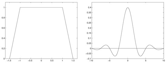
Figure 1. Piecewise linear characteristic function (left) and corresponding kernel (right), $c=1.5$.

The second case refers to the infinitely differentiable flat-top kernel characteristic function defined in [28], i.e.,

$$\lambda (s)=\left\{\begin{array}{cc}1,\hfill & \left|s\right|\le c,\hfill \\ exp\left[-bexp\left[-b/{(|s|-c)}^2\right]/{(|s|-1)}^2\right],\hfill & c<\left|s\right|<1,\hfill \\ 0,\hfill & \left|s\right|\ge 1.\hfill \end{array}\right.$$

The characteristic function and kernel of the second case are shown in Figure 2.

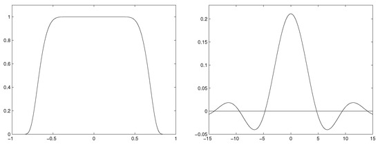
Figure 2. Infinitely differentiable flat-top characteristic function (left) and corresponding kernel (right), $c=0.05$, $b=1$.

We examine kernel density estimators of triangular, exponential, Laplace, and gamma (with various shape parameter) distributions. Figure 3, Figure 4 and Figure 5 illustrate the estimator MSE as a function of the sample size.

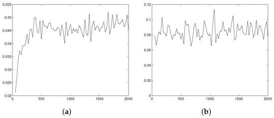
Figure 3. MSE of kernel estimators multiplied by $n^{3/4}$ as a function of the sample size n for the triangle density function. (a) MSE of estimator with piecewise linear kernel characteristic function. (b) MSE of estimator with infinitely differentiable flat-top kernel characteristic function.

Figure 4. MSE of kernel estimators (with piecewise linear kernel characteristic function) as a function of the sample size n. (a) Laplace density function ($r=1$, MSE multiplied by $n^{3/4}$). (b) Gamma density function ($k=3$, $r=2$, MSE multiplied by $n^{5/6}$).

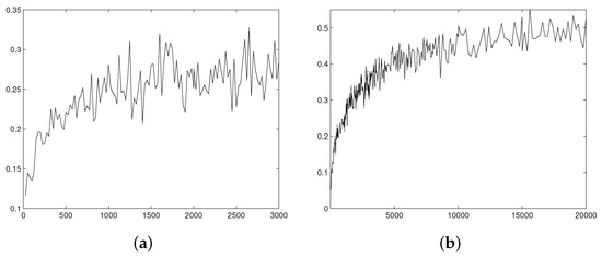
Figure 5. MSE of kernel estimators (with piecewise linear kernel characteristic function) as a function of the sample size n. (a) Gamma distribution shape parameter $k=4$, $r=3$ (MSE multiplied by $n^{7/8}$). (b) Gamma distribution shape parameter $k=6$, $r=5$ (MSE multiplied by $n^{11/12}$).

Using notation $C(x)=\{0,x<0;1,x\ge 0\}$ for Heaviside step function, the triangular density function is defined as $f(x)=((\lambda -\left|x\right|)/{\lambda }^2)C(\lambda -x)C(\lambda +x)$ having characteristic function $\varphi (s)=2(1-cos(\lambda s))/{(\lambda s)}^2.$ Laplace density $f(x)=\lambda /2exp(-\lambda |x|)$ has characteristic function $\varphi (s)={\lambda }^2/({\lambda }^2+s^2)$, gamma density $f(x)={\lambda }^k{x}^{k-1}{e}^{-\lambda x}/\mathsf{\Gamma }(k)$ has characteristic function $\varphi (s)={\lambda }^k/{(\lambda -is)}^k$.

In all cases we choose scale parameter $\lambda$ to have variation equals to 1, and consider estimation of density function $f(x)$ at point $x=1$.

All the above-mentioned characteristic functions $\varphi (s)$ satisfy condition (4) for $r=1$ (triangular and Laplace), and $r=k-1$ (gamma, $k>1$); therefore, all distributions belong to the family ${\mathcal{F}}_r$ with corresponding value of r. In addition, all $\varphi (s)$ meet the requirements of Example 2. Thus, the bandwidth can be taken in the form $h=O(n^{-1/(2(r+1))})$ and the expected convergence rate of the kernel estimator MSE is $n^{-(2r+1)/(2(r+1))}.$

The main goal of the simulation study is investigation of the MSE behavior for the kernel estimator with the growth of sample size. We generate sequences of 150 samples for sample size from 25 to 2000 with step 25, and for some distributions for sample size from 2000 to 20,000 with step 100 or 200. Then, for each sample size we calculate the estimator MSE multiplied by $n^{-(2r+1)/(2(r+1))}$ and expect visual stabilization of the sequence of resulting values with growth of $n.$

Typical examples of the simulation results are presented at Figure 3 (for $r=1$), Figure 4 (for $r=1$ and $r=2$), and Figure 5 (for $r=3$ and $r=5$). The expected stabilization of the scaled MSE is observed in all cases. Moreover, increasing r causes enlargement of sample size that is needed to achieve limiting asymptotic behavior. For $r=1$ and $r=2$ we can see stabilization starting from $n\approx 500$, for $r=3$ it starts from $n\approx 1500$, while for $r=5$ the asymptotic behavior is observed to start from sample size $n\approx$ 15,000.

7. Technical Proofs

7.1. Proof of Lemma 1

First we note that for every $m\ge 1$ and $n\ge 1$ there exist positive numbers ${\kappa }_m$ such that

$${\displaystyle \underset{f\in {\overline{\mathcal{F}}}_r}{sup}{E}_f{|{\varphi }_n(s)-\varphi (s)|}^{2m}\le \frac{{\kappa }_m}{n^m}.}$$

These inequalities follow from the Burkholder inequality (see, for example, [29]) for the martingale $({\displaystyle \sum _{k=1}^n}({\mathrm{e}}^{is{X}_k}-\varphi (s)),{\mathcal{F}}_n^X),$ ${\mathcal{F}}_n^X=\sigma \{X_1,\dots ,X_n\}$ and finiteness of the function $\varphi (·).$

Using this and Hölder’s inequalities we can estimate

$$\underset{f\in {\overline{\mathcal{F}}}_r}{sup}{E}_f{J}_{n,\alpha }^{2m}=\underset{f\in {\overline{\mathcal{F}}}_r}{sup}{E}_f{\left[\underset{A_n<\left|s\right|<B_n}{\int }{\left|s\right|}^{\alpha }|{\varphi }_n(s)-\varphi (s)|ds\right]}^{2m}$$

$$\le {\left(\underset{A_n<\left|s\right|<B_n}{\int }{\left|s\right|}^{\frac{2m\alpha }{2m-1}}ds\right)}^{2m-1}·\underset{A_n<\left|s\right|<B_n}{\int }\underset{f\in {\overline{\mathcal{F}}}_r}{sup}{E}_f{|{\varphi }_n(s)-\varphi (s)|}^{2m}ds\le \frac{C_{\alpha ,m}{B}_n^{2m(\alpha +1)}}{n^m}.$$

From the Borel–Cantelli lemma and the assumed summability of the right-hand side of (13) for $m=m_0,\alpha ={\varrho }_n+{\delta }_n$ and $f\in {\overline{\mathcal{F}}}_r$ follows the second assertion of Lemma 1.

7.2. Proof of Theorem 2

We prove now the statements $1^{\circ }$ (a) and $2^{\circ }$ (a) of Theorem 1. First, we show for n large enough the inequalities

$$r_n^{+}<{\varrho }_n{P}_f-\mathrm{a}.\mathrm{s}.$$

(18)

To this end, according to the definition of the estimator $r_n^{+},$ it is enough to establish for some $\alpha >r$ the limiting relation

$$\underset{n\to \infty }{lim}{\mathsf{\Phi }}_{n,\alpha }(A_n,B_n)=\infty P_f-\mathrm{a}.\mathrm{s}.,$$

which follows from the definition of the class ${\mathcal{C}}_{+}$ and Lemma 1:

$$\begin{gathered} {\mathsf{\Phi }}_{n,\alpha }(A_n,B_n)={\mathsf{\Phi }}_{n,\alpha }(A_n,B_n)-{\mathsf{\Phi }}_{\alpha }(A_n,B_n)+{\mathsf{\Phi }}_{\alpha }(A_n,B_n) \\ \ge {\mathsf{\Phi }}_{\alpha }(A_n,B_n)-J_{n,\alpha }\to \infty P_f-\mathrm{a}.\mathrm{s}. \end{gathered}$$

From (18) and by the definition of the estimator $r_n^{+},$ for n large enough, we have

$${\mathsf{\Phi }}_{n,r_n^{+}+{\delta }_n}(A_n,B_n)\ge H.$$

Thus,

$$\underset{\overline{n\to \infty }}{lim}{\mathsf{\Phi }}_{r_n^{+}+{\delta }_n}(A_n,B_n)\ge \underset{\overline{n\to \infty }}{lim}{\mathsf{\Phi }}_{n,r_n^{+}+{\delta }_n}(A_n,B_n)$$

$$-\overline{\underset{n\to \infty }{lim}}{J}_{n,{\varrho }_n+{\delta }_n}\ge H{P}_f-\mathrm{a}.\mathrm{s}.$$

(19)

Analogously,

$$\overline{\underset{n\to \infty }{lim}}{\mathsf{\Phi }}_{r_n^{+}}(A_n,B_n)\le H{P}_f-\mathrm{a}.\mathrm{s}.$$

(20)

From (19) and (20) it follows, that for any $\epsilon >0$ and $\delta >0$ for n large enough

$$r-\epsilon -\delta <r_n^{+}<r+\epsilon P_f-\mathrm{a}.\mathrm{s}.$$

and the assertion 1(a) of Theorem 2 is proved.

From the definitions of the estimator $r_n^{+},$ class ${\mathcal{C}}_{+}^{*},$ Chebyshev’s inequality and (13), for $m\ge 1,n>n_1$ and $f\in {\mathcal{F}}_r^{+}$ we have

$$P_f(r_{n-1}^{+}<r-{\delta }_{n-1})\le P_f({\mathsf{\Phi }}_{n,r}(A_n,B_n)\ge H)\le P_f(J_{n,r}\ge H-{\mathsf{\Phi }}_r(A_n,B_n))$$

$$\le \frac{E_f{J}_{n,r}^{2m}}{{(H-{\mathsf{\Phi }}_r(A_n,B_n))}^{2m}}\le \frac{C_{r,m}{B}_n^{2m(r+1)}}{n^m}.$$

(21)

Similar to (21) for $n>n_2$ and $m\ge 1$ we obtain

$$\begin{gathered} P_f(r_{n-1}^{+}>r+{\delta }_{n-1})\le P_f({\mathsf{\Phi }}_{n,r+{\delta }_n}(A_n,B_n)<H)=P_f({\mathsf{\Phi }}_{r+{\delta }_n}(A_n,B_n)-H\le J_{n,r+{\delta }_n}) \\ \le \frac{E_f{J}_{n,r+{\delta }_n}^{2m}}{{({\mathsf{\Phi }}_{r+{\delta }_n}(A_n,B_n)-H)}^{2m}}\le \frac{C_{r+1,m}{B}_n^{2m(r+1+{\delta }_n)}}{n^m} \end{gathered}$$

(22)

and, as follows, for $f\in {\mathcal{F}}_r^{+},$

$$P_f({\delta }_n^{-1}|r_n^{+}-r|\ge 1)\le \frac{2C_{r+1,m}{B}_n^{2m(r+1+{\delta }_n)}}{n^m}.$$

(23)

From the Borel–Cantelli lemma and the assumed summability of the right hand side in (23) for $m\ge m_0$ follows the assertion 2(a) of Theorem 2.

The other statements of Theorem 2 for the estimator $r_n$ can be proved analogically.

7.3. Proof of Theorem 3

Consider the deviation of the estimator (14) in the following form:

$${\widehat{f}}_n(x)-f(x)=I_1(n)+I_2(n),$$

(24)

where

$$I_1(n)={\widehat{f}}_n(x)-{\tilde{f}}_n(x),I_2(n)={\tilde{f}}_n(x)-f(x),$$

$${\tilde{f}}_n(x)=\frac{1}{n}\sum _{j=1}^n\int K(z)f(x-{\widehat{h}}_{j-1}z)dz=\frac{1}{2\pi n}\sum _{j=1}^n\int {\lambda }_{j-1}(s)\varphi (s){\mathrm{e}}^{-isx}ds.$$

Now we estimate second moments of $I_1(n)$ and $I_2(n).$ Denote ${\mathcal{F}}_j^X=\sigma \{X_1,\dots ,X_j\}.$ For $f\in {\overline{\mathcal{F}}}_r$ we have

$$E_f{I}_1^2(n)=\frac{1}{n^2}{E}_f{\left(\sum _{j=1}^n\frac{1}{{\widehat{h}}_{j-1}}\left[K\left(\frac{x-X_j}{{\widehat{h}}_{j-1}}\right)-{\widehat{h}}_{j-1}\int K(z)f(x-{\widehat{h}}_{j-1}z)dz\right]\right)}^2$$

$$=\frac{1}{n^2}{E}_f\sum _{j=1}^n\frac{1}{{\widehat{h}}_{j-1}^2}{E}_f\left({\left[K\left(\frac{x-X_j}{{\widehat{h}}_{j-1}}\right)-{\widehat{h}}_{j-1}\int K(z)f(x-{\widehat{h}}_{j-1}z)dz\right]}^2|{\mathcal{F}}_{j-1}^X\right)$$

$$=\frac{1}{n^2}{E}_f\sum _{j=1}^n\frac{1}{{\widehat{h}}_{j-1}}\int {[K(u)-{\widehat{h}}_{j-1}\int K(z)f(x-{\widehat{h}}_{j-1}z)dz]}^{2}f(x-{\widehat{h}}_{j-1}u)du$$

$$\le \frac{C_1}{n^2}\sum _{j=1}^n{E}_f\frac{1}{{\widehat{h}}_{j-1}}+\frac{{\overline{f}}^2}{n}\le \frac{C_1}{n^2}\sum _{j=1}^n\frac{1}{h_{j-1}^{*}}+\frac{C_1}{n^2}\sum _{j=1}^{n}j{P}_f(r(j)<r-{\delta }_j)+\frac{{\overline{f}}^2}{n}.$$

From (21) for $m=2m_0$ we obtain

$$E_f{I}_1^2(n)\le \frac{C_1}{n^2}\sum _{j=1}^n\frac{1}{h_{j-1}^{*}}+\frac{C_1}{n^2}\sum _{j=1}^{n_1}j+\frac{C_1{C}_{r,2m_0}}{n^2}\sum _{j>n_1}\frac{j{B}_j^{4m_0(r+1)}}{j^{2m_0}}+\frac{{\overline{f}}^2}{n}$$

$$=\frac{C_1}{n^2}\sum _{j=1}^n\frac{1}{h_{j-1}^{*}}+\frac{{\tilde{C}}_1}{n^2}+\frac{{\overline{f}}^2}{n}.$$

(25)

Further, by the definition of the function $\tilde{f}(x),$ the Cauchy–Bunyakovskii–Schwarz inequality and from (22) we have

$$\begin{gathered} E_f{I}_2^2(n)=\frac{1}{4{\pi }^2{n}^2}{E}_f{\left[\sum _{j=1}^n\underset{\left|s\right|\ge {\widehat{h}}_{j-1}^{-1}}{\int }({\lambda }_{j-1}(s)-1)\varphi (s){\mathrm{e}}^{-isx}ds\right]}^2 \\ \le \frac{1}{4{\pi }^{2}n}\sum _{j\ge 1}{E}_f{\left[\underset{\left|s\right|\ge {\widehat{h}}_{j-1}^{-1}}{\int }\left|\varphi (s)\right|ds\right]}^2\le \frac{1}{4{\pi }^{2}n}\sum _{j=1}^n{E}_f{\widehat{h}}_{j-1}^{2r-2\gamma }·{\left[\underset{\left|s\right|\ge {\widehat{h}}_{j-1}^{-1}}{\int }{\left|s\right|}^{r-\gamma }\left|\varphi (s)\right|ds\right]}^2 \\ =\frac{1}{4{\pi }^{2}n}\sum _{j=1}^n{E}_f{\widehat{h}}_{j-1}^{2r-2\gamma }{\Delta }_{\gamma }^2({\widehat{h}}_{j-1})\le \frac{1}{4{\pi }^{2}n}\left[\sum _{j=1}^n{\tilde{h}}_{j-1}^{2r-2\gamma }{\Delta }_{\gamma }^2({\tilde{h}}_{j-1})+\sum _{j=1}^{n_2}{\overline{h}}_{j-1}^{2r-2\gamma }{\Delta }_{\gamma }^2({\overline{h}}_{j-1})\right. \\ \left.+\sum _{j>n_2}{\overline{h}}_{j-1}^{2r-2\gamma }{\Delta }_{\gamma }^2({\overline{h}}_{j-1})P_f(r(j)>r-\gamma +{\delta }_j)\right]\le \frac{1}{4{\pi }^{2}n}\left[\sum _{j=1}^n{\tilde{h}}_{j-1}^{2r-2\gamma }{\Delta }_{\gamma }^2({\tilde{h}}_{j-1})\right. \\ \left.+\sum _{j=1}^{n_2}{\overline{h}}_{j-1}^{2r-2\gamma }{\Delta }_{\gamma }^2({\overline{h}}_{j-1})+C_{r+1,m_0}\sum _{j>n_2}{\overline{h}}_{j-1}^{2r-2\gamma }{\Delta }_{\gamma }^2({\overline{h}}_{j-1})\frac{B_j^{2m_0(r+1+{\delta }_j)}}{n^{m_0}}\right] \\ \le \frac{1}{4{\pi }^{2}n}\sum _{j=1}^n{\tilde{h}}_{j-1}^{2r-2\gamma }{\Delta }_{\gamma }^2({\tilde{h}}_{j-1})+\frac{C_2}{n}. \end{gathered}$$

(26)

From (24)–(26) follows the first assertion of Theorem 3.

For the proof of the second assertion we estimate first, for some integer $m>1$ the rate of convergence of the moment $E_f{I}_1^{2m}(n).$

Let ${\alpha }_1,\dots ,{\alpha }_m$ be non-negative integers and denote

$${\tilde{K}}_j(x)=K\left(\frac{x-X_j}{{\widehat{h}}_{j-1}}\right)-{\widehat{h}}_{j-1}\int K(z)f(x-{\widehat{h}}_{j-1}z)dz,$$

$${\overline{K}}_j(x)=\int {[K(u)-{\widehat{h}}_{j-1}\int K(z)f(x-{\widehat{h}}_{j-1}z)dz]}^{2}f(x-{\widehat{h}}_{j-1}u)du.$$

By the Burkholder inequality for the martingale ${\displaystyle \sum _{j=1}^n}\frac{1}{{\widehat{h}}_{j-1}}{\tilde{K}}_j(x)$ we have

$${\displaystyle E_f{I}_1^{2m}(n)=\frac{1}{n^{2m}}{E}_f{\left(\sum _{j=1}^n\frac{1}{{\widehat{h}}_{j-1}}{\tilde{K}}_j(x)\right)}^{2m}\le \frac{C}{n^{2m}}{E}_f{\left(\sum _{j=1}^n\frac{1}{{\widehat{h}}_{j-1}^2}{\tilde{K}}_j^2(x)\right)}^m}$$

$${\displaystyle \le \frac{C}{n^{2m}}\sum _{{\alpha }_1+\dots +{\alpha }_m=m}\sum _{1\le j_1<\dots <j_m\le n}{E}_f\frac{1}{{\widehat{h}}_{j_1-1}^2·\dots ·{\widehat{h}}_{j_m-1}^2}{\tilde{K}}_{j_1}^2(x)·\dots ·{\tilde{K}}_{j_m}^2(x)}$$

$${\displaystyle \le \frac{C}{n^{2m}}\sum _{{\alpha }_1+\dots +{\alpha }_m=m}\sum _{1\le j_1<\dots <j_m\le n}{E}_f\frac{{\tilde{K}}_{j_1}^2(x)·\dots ·{\tilde{K}}_{j_{m-1}}^2(x)·{\overline{K}}_{j_m}(x)}{{\widehat{h}}_{j_1-1}^2·\dots ·{\widehat{h}}_{j_{m-1}-1}^2·h_{j_m-1}^{*}}}$$

$${\displaystyle \le \frac{C}{n^{2m}}\sum _{{\alpha }_1+\dots +{\alpha }_m=m}\sum _{1\le j_1<\dots <j_m\le n}{E}_f\frac{1}{{\widehat{h}}_{j_1-1}^2·\dots ·{\widehat{h}}_{j_{m-2}-1}^2·h_{j_{m-1}-1}^{*}·h_{j_m-1}^{*}}}$$

$${\displaystyle ·{\tilde{K}}_{j_1}^2(x)·\dots ·{\tilde{K}}_{j_{m-2}}^2(x)·{\overline{K}}_{j_{m-1}}(x)\le \dots \le \frac{C}{n^{2m}}{\left(\sum _{j=1}^n\frac{1}{h_{j-1}^{*}}\right)}^m.}$$

By the definition of $h_j^{*}$ for some $0<r_{*}<r-\gamma$ and $j_{*}<\infty ,$$h_j^{*}\ge n^{-\frac{1}{1+2r_{*}}}$ and, as follows

$${\displaystyle E_f{I}_1^{2m}(n)=O\left(n^{-\frac{2m{r}_{*}}{1+2r_{*}}}\right)\mathrm{as}n\to \infty .}$$

Thus ${\displaystyle \frac{2m{r}_{*}}{1+2r_{*}}>1}$ for ${\displaystyle m>\frac{1+2r_{*}}{2r_{*}}}$ and by the Borel–Cantelli lemma, as $n\to \infty ,$

$$I_1(n)\to 0P_f-\mathrm{a}.\mathrm{s}.$$

(27)

Further,

$$|I_2(n)|\le \frac{1}{4{\pi }^{2}n}\sum _{j=1}^n{\widehat{h}}_{j-1}^r\left|{\Delta }_{\gamma }({\widehat{h}}_{j-1})\right|$$

and, as follows, as $n\to \infty ,$

$$I_2(n)\to 0P_f-\mathrm{a}.\mathrm{s}.$$

(28)

From (27) and (28) follows the second assertion of Theorem 3.

7.4. Proof of Theorem 4

Note that the distribution of ${\widehat{f}}_n^{(k)}(x)$ is the same as that of ${\widehat{f}}_n^{(j)}(x)$ for all $k,j$. Hence, $E{\overline{f}}_{n,b}(x)=E{\widehat{f}}_n(x).$ Now $|Cov({\widehat{f}}_n^{(k)}(x),{\widehat{f}}_n^{(j)}(x))|\le Var({\widehat{f}}_n^{(1)}(x))$ by the Cauchy–Schwarz inequality and the fact that $Var({\widehat{f}}_n^{(k)}(x))=Var({\widehat{f}}_n^{(j)}(x))$. Thus,

$$Var({\overline{f}}_{n,b}(x))=\frac{1}{b^2}\sum _{k=1}^b\sum _{j=1}^{b}Cov({\widehat{f}}_n^{(k)}(x),{\widehat{f}}_n^{(j)}(x))\le Var({\widehat{f}}_n^{(1)}(x))$$

and the theorem is proven.

8. Conclusions

Non-parametric kernel estimation crucially depends on the bandwidth choice which, in turn, depends on the smoothness of the underlying function. Focusing on estimating a probability density function, we define a smoothness class and propose a data-based estimator of the underlying degree of smoothness. The convergence rates in the almost sure sense of the proposed estimators are obtained. Adaptive estimators of densities from the given class on the basis of the constructed smoothness parameter estimators are also presented, and their consistency is established. Simulation results illustrate the realization of the asymptotic behavior when the sample size grows large.

Recently, there has been an increasing interest in nonparametric estimation with dependent data both in terms of theory as well as applications; see, e.g., [15,30,31,32,33]. With respect to probability density estimation, many asymptotic results remain true when moving from i.i.d. data to data that are weakly dependent. For example, the estimator variance, bias and MSE have the same asymptotic expansions as in the i.i.d. case subject to some limitations on the allowed bandwidth rate; fortunately, the optimal bandwidth rate of $n^{-1/5}$ is in the allowed range—see [34,35].

Consequently, it is conjectured that our proposed estimator of smoothness—as well as resulting data-based bandwidth choice and probability density estimator—will retain their validity even when the data are weakly dependent. Future work may confirm this conjecture especially since working with dependent data can be quite intricate. For example, [36] extended the results of [34] from the realm of linear time series to strong-mixing process. In so doing, Remark 5 of [36] pointed to a nontrivial error in the work of [34] which is directly relevant to optimal bandwidth choice.

References

- Rosenblatt, M. Stochastic Curve Estimation; NSF-CBMS Regional Conference Series in Probability and Statistics, 3; Institute of Mathematical Statistics: Hayward, CA, USA, 1991. [Google Scholar]
- Bartlett, M.S. Statistical estimation of density function. Sankhya Indian J. Stat. 1963, A25, 245–254. [Google Scholar]
- Parzen, E. On estimation of a probability density function and mode. Ann. Math. Stat. 1962, 33, 1065–1076. [Google Scholar] [CrossRef]
- Devroye, L. A Course in Density Estimation; Birkhäuser: Boston, MA, USA; Basel, Switzerland; Stuttgart, Germany, 1987. [Google Scholar]
- Gasser, T.; Müller, H.-G.; Mammitzsch, V. Kernels for nonparametric curve estimation. J. R. Stat. Soc. Ser. B 1985, 60, 238–252. [Google Scholar] [CrossRef]
- Granovsky, B.L.; Müller, H.-G. Optimal kernel methods: A unifying variational principle. Int. Stat. Rev. 1991, 59, 373–388. [Google Scholar] [CrossRef]
- Jones, M.C. On higher order kernels. J. Nonparametric Stat. 1995, 5, 215–221. [Google Scholar] [CrossRef]
- Marron, J.S. Visual understanding of higher order kernels. J. Comput. Graph. Stat. 1994, 3, 447–458. [Google Scholar]
- Müller, H.-G. Nonparametric Regression Analysis of Longitudinal Data; Springer: Berlin/Heidelberg, Germany, 1988. [Google Scholar]
- Scott, D.W. Multivariate Density Estimation: Theory, Practice and Visualization; Wiley: New York, NY, USA, 1992. [Google Scholar]
- Devroye, L. A note on the usefulness of superkernels in density estimation. Ann. Stat. 1992, 20, 2037–2056. [Google Scholar] [CrossRef]
- Politis, D.N. On nonparametric function estimation with infinite-order flat-top kernels. In Probability and Statistical Models with Applications; Charalambides, C., Ed.; Chapman and Hall/CRC: Boca Raton, FL, USA, 2001; pp. 469–483. [Google Scholar]
- Jones, M.C.; Marron, J.S.; Sheather, S.J. A brief survey of bandwidth selection for density estimation. J. Am. Stat. Assoc. 1996, 91, 401–407. [Google Scholar] [CrossRef]
- Tsybakov, A. Introduction to Nonparametric Estimation; Springer Series in Statistics; Springer: New York, NY, USA, 2009. [Google Scholar]
- Dobrovidov, A.V.; Koshkin, G.M.; Vasiliev, V.A. Non-Parametric State Space Models; Kendrick Press: Heber City, UT, USA, 2012. [Google Scholar]
- Ibragimov, I.A.; Khasminskii, R.Z. Statistical Estimation: Asymptotic Theory; Springer: Berlin/Heidelberg, Germany, 1981. [Google Scholar]
- Lehmann, E.L.; Romano, J.P. Testing Statistical Hypotheses, 4th ed.; Springer Texts in Statistics: New York, NY, USA, 2022. [Google Scholar]
- Lepskii, O.V.; Spokoiny, V.G. Optimal pointwise adaptive methods in nonparametric estimation. Ann. Stat. 1997, 25, 2512–2546. [Google Scholar] [CrossRef]
- Brown, L.D.; Low, M.G. Superefficiency and Lack of Adaptibility in Functional Estimation; Technical Report; Cornell University: Ithaca, NY, USA, 1992. [Google Scholar]
- Lepskii, O.V. On a problem of adaptive estimation in Gaussian white noise. Theory Probab. Its Appl. 1990, 35, 454–466. [Google Scholar] [CrossRef]
- Butucea, C. Exact adaptive pointwise estimation on Sobolev classes of densities. ESAIM Probab. Stat. 2001, 5, 1–31. [Google Scholar] [CrossRef]
- Goldenshluger, A.; Lepski, O. Bandwidth selection in kernel density estimation: Oracle inequalities and adaptive minimax optimality. Ann. Statist. 2011, 39, 1608–1632. [Google Scholar] [CrossRef]
- Lacour, C.; Massart, P.; Rivoirard, V. Estimator selection: A new method with applications to kernel density estimation. Sankhya A 2017, 79, 298–335. [Google Scholar] [CrossRef]
- Politis, D.N. Adaptive bandwidth choice. J. Nonparametric Stat. 2003, 15, 517–533. [Google Scholar] [CrossRef]
- Politis, D.N.; Romano, J.P. On a Family of Smoothing Kernels of Infinite Order. In Computing Science and Statistics, Proceedings of the 25th Symposium on the Interface, San Diego, CA, USA, 14–17 April 1993; Tarter, M., Lock, M., Eds.; The Interface Foundation of North America: San Diego, CA, USA, 1993; pp. 141–145. [Google Scholar]
- Politis, D.N.; Romano, J.P. Multivariate density estimation with general flat-top kernels of infinite order. J. Multivar. Anal. 1999, 68, 1–25. [Google Scholar] [CrossRef]
- Politis, D.N.; Romano, J.P.; Wolf, M. Subsampling; Springer: New York, NY, USA, 1999. [Google Scholar]
- McMurry, T.; Politis, D.N. Nonparametric regression with infinite order flat-top kernels. J. Nonparametric Stat. 2004, 16, 549–562. [Google Scholar] [CrossRef]
- Liptser, R.; Shiryaev, A. Theory of Martingales; Springer: New York, NY, USA, 1988. [Google Scholar]
- Bijloos, G.; Meyers, J.A. Fast-Converging Kernel Density Estimator for Dispersion in Horizontally Homogeneous Meteorological Conditions. Atmosphere 2021, 12, 1343. [Google Scholar] [CrossRef]
- Cortes Lopez, J.C.; Jornet Sanz, M. Improving Kernel Methods for Density Estimation in Random Differential Equations Problems. Math. Comput. Appl. 2020, 25, 33. [Google Scholar] [CrossRef]
- Correa-Quezada, R.; Cueva-Rodriguez, L.; Alvarez-Garcia, J.; del Rio-Rama, M.C. Application of the Kernel Density Function for the Analysis of Regional Growth and Convergence in the Service Sector through Productivity. Mathematics 2020, 8, 1234. [Google Scholar] [CrossRef]
- Vasiliev, V.A. A truncated estimation method with guaranteed accuracy. Ann. Inst. Stat. Math. 2014, 66, 141–163. [Google Scholar] [CrossRef]
- Hallin, M.; Tran, L.T. Kernel density estimation for linear processes: Asymptotic normality and bandwidth selection. Ann. Inst. Stat. Math. 1996, 48, 429–449. [Google Scholar] [CrossRef]
- Wu, W.-B.; Mielniczuk, J. Kernel density estimation for linear processes. Ann. Stat. 2002, 30, 1441–1459. [Google Scholar] [CrossRef]
- Lu, Z. Asymptotic normality of kernel density estimators under dependence. Ann. Inst. Stat. Math. 2001, 53, 447–468. [Google Scholar] [CrossRef]
Disclaimer/Publisher’s Note: The statements, opinions and data contained in all publications are solely those of the individual author(s) and contributor(s) and not of MDPI and/or the editor(s). MDPI and/or the editor(s) disclaim responsibility for any injury to people or property resulting from any ideas, methods, instructions or products referred to in the content. |
© 2022 by the authors. Licensee MDPI, Basel, Switzerland. This article is an open access article distributed under the terms and conditions of the Creative Commons Attribution (CC BY) license (https://creativecommons.org/licenses/by/4.0/).