Study of the ρ⁰ Decay into π⁰π⁰γ Within Framework of Chiral Perturbation Theory with Resonances

Abstract

In this work, we calculate the Branching Ratio (BR) of the process ${\rho }^0\to {\pi }^0{\pi }^0\gamma$ at tree level within the theoretical framework of with resonances, including the odd intrinsic parity sector. Owing to the nature of an effective field theory, the BR depends on three unknown couplings of the model: $d_4$ and the combination $c_{57}=c_5+c_7$. To constrain these unknown couplings, we use the experimental BR of this decay and explore the possibility of reducing the number of unknown couplings through the on-shell condition at one vertex. Our result suggests that off-shell conditions must be applied to both vertices, leading to a space parameter for the pair ($c_{57},d_4$).

1. Introduction

The Standard Model (SM) of particle physics [1,2] is one of the most successful theories; it predicts almost all phenomena in particle physics between matter and its interactions: electromagnetic, weak, and strong. However, it is incomplete because it does not incorporate dark matter, gravity, and neutrino masses, and it does not explain the asymmetry of matter–antimatter in the universe. Nowadays, SM is considered an effective field theory with 19 free parameters that cannot be derived from the theory itself. Instead, these parameters must be determined phenomenologically, which is accomplished through the advancement of particle collider experiments. The current status of these parameters can be found in Ref. [3].

At low energies, i.e., below 1 GeV, the particle spectrum consists predominantly of hadrons, which are composed of quarks embedded in a gluon sea. Gluons are the massless gauge bosons of spin 1 that mediate the strong interactions between quarks. In this regime, the strong coupling constant ${\alpha }_s$ becomes sufficiently large to prevent the use of perturbative methods. Consequently, the hadronic structure dynamics cannot be described within the framework of SM at such energy scales.

As an alternative approach to the study of strong interactions, Effective Field Theories (EFTs) provide an ideal framework. They are constructed from the underlying fundamental theory in accordance with Weinberg’s theorem [4], which states that the effective Lagrangian must respect the symmetries relevant to the energy range of interest. However, the predictive power of an EFT relies on our knowledge of its Low Energy Coupling constants (LECs), which cannot be determined by symmetry requirements and must therefore be obtained either from the underlying theory or through phenomenological methods.

Chiral Perturbation Theory (ChPT) is an EFT of Quantum Chromodynamics (QCD) in the chiral limit (the chiral limit denotes the theoretical scenario in which the light quarks u, d, and s are massless), formulated as a perturbative expansion in powers of momenta. The relevant degrees of freedom correspond to the Goldstone bosons arising from the spontaneous breaking of chiral symmetry, which can be identified with the lightest pseudoscalar mesons [5]. At leading order, corresponding to $\mathcal{O}\left(p^2\right)$, the effective Lagrangian depends on two LECs, whose values are determined phenomenologically and are well established [5,6]. However, at higher orders, such as $\mathcal{O}\left(p^4\right)$, the number of LECs increases significantly, making their determination a challenge.

As the energy increases up to 1 GeV, the role of resonance particles becomes significant, and they must be included as additional degrees of freedom. This leads to the framework of Resonance Chiral Theory ($R\chi T$) [6,7], which introduces new LECs. In the even parity sector [7], two LECs arise, and their corresponding values are well known. On the other hand, the odd intrinsic parity sector, formulated in Ref. [8], includes interactions between two light resonances (vectors) and one light pseudoscalar field, namely, the VVP operators. Moreover, the interaction involving a vector, a pseudoscalar, and an external source (VJP) allows one to describe electromagnetic and weak interactions. This formulation incorporates eleven LECs, which are a priori unknown. Fortunately, by constructing the Green’s three-point functions of the VVP and VJP in leading order in $1/{\mathrm{N}}_{\mathrm{c}}$, some combinations of these LECs can be predicted if the short-distance (high-energy) behavior of these Green’s functions matches the corresponding Operator Product Expansion (OPE) [8]. Nonetheless, some couplings remain unknown, in particular, $c_5,c_7$, and $d_4$, thus requiring a phenomenological analysis to set reasonable bounds on LECs.

In computing the Isospin Symmetry-Breaking (IB) effects in the process ${\tau }^{+}\to {\pi }^{+}{\pi }^0{\overline{\nu }}_{\tau }$, an upper bound of $\left|d_4\right|<0.15$ is assumed in Ref. [9]. These IB corrections are important in the tau-based determination of the hadronic vacuum polarization contribution to the anomalous magnetic moment of the muon [10]. Following the same line, Ref. [11] found that the ${\omega }^0\to {\pi }^0{\pi }^0\gamma$ decay can provide information on $d_4$, assuming the on-shell condition for the ${\rho }^0{\omega }^0{\pi }^0$ vertex, which eliminates the $c_5,c_7,$ dependence. This coupling is an input in the authors’ analysis of the triple-product asymmetries in the $\tau$ decay and in the radiative two-pion decay, namely, ${\tau }^{+}\to {\pi }^{+}{\pi }^0{\nu }_{\tau }\gamma$. They report two possible values, $d_4=0.82\pm 0.05$ and $d_4=-0.12\pm 0.05$, and choose (see discussion in Appendix B of Ref. [11]) the positive one in their analysis to maintain consistency with the result in [9].

With this proviso, it is clear that a more general analysis of this pair of couplings can be performed. The aim of this work is to determine the values of these couplings through the analysis of the branching ratio $\mathcal{BR}({\rho }^0\to {\pi }^0{\pi }^0\gamma )$, described at tree level within the framework of the odd intrinsic parity Lagrangian, considering both vertices to be off-shell.

This paper is organized as follows. In Section 2, we review the foundations of (ChPT) and the inclusion of light resonances that give rise to $R\chi T$, covering both the even- and odd-intrinsic-parity sectors, as described in Ref. [8]. In Section 3, we compute the invariant amplitude of the process ${\rho }^0\to {\pi }^0{\pi }^0\gamma$, showing that it only depends on $c_{57}\equiv c_5+c_7$ and $d_4$. In addition, the on-shell and off-shell vertices are defined, and their impact on the determination of the BR is discussed. In Section 4, we present our results and conclusions, and in the last section, Appendix A, the full analytical expressions are reported.

2. Chiral Perturbation Theory with Resonances

ChPT is an EFT of QCD that incorporates all the essential features of QCD at low energies—well below 1 GeV. It is formulated as an expansion in powers of momentum, where the relevant degrees of freedom are the eight Goldstone bosons corresponding to the lightest states in the hadronic spectrum. According to the power-counting scheme, the ChPT Lagrangian, at lowest order $\mathcal{O}\left(p^2\right)$, is given by

$${\mathcal{L}}_{\chi }^{\left(2\right)}={\displaystyle \frac{F^2}{4}}Tr\left(D_{\mu }{U}^{†}{D}^{\mu }U+U^{†}\chi +{\chi }^{†}U\right),$$

(1)

where Tr denotes the trace and

$$U\left(\varphi \right)=exp\left(i{\displaystyle \frac{\sqrt{2}\varphi }{F}}\right),$$

(2)

is the parameterization of the Goldstone fields ${\varphi }_a$, which transform under the group (the symmetry group $G:=SU{\left(3\right)}_L\times SU{\left(3\right)}_R$ is referred to as the chiral symmetry) G as

$$U\stackrel{G}{\to }{g}_{R}U{g}_L^{†},g\equiv (g_L,g_R)\in G.$$

(3)

The field $\varphi$ is expressed as follows:

$$\varphi =\sum _{a=1}^8{\varphi }_a{\displaystyle \frac{{\lambda }_a}{\sqrt{2}}},$$

(4)

where ${\lambda }_a$ denotes the Gell-Mann matrices, and the covariant derivative

$$D_{\mu }U={\partial }_{\mu }U-i{r}_{\mu }U+iU{\ell }_{\mu },$$

(5)

is determined to transform as

$$D_{\mu }U\left(x\right)⟶g_R\left(D_{\mu }U\right)g_L^{†}.$$

(6)

The symmetry breaking is introduced by the last two terms in Equation (1) with

$$\chi =2B_0(s+ip),$$

(7)

where s and p are the scalar and pseudoscalar external fields, respectively.

The constants F and $B_0$ are LECs that can be determined phenomenologically [5,8]. For instance, $F\approx F_{\pi }=92.4\mathrm{MeV}$ is associated with the pion decay constant, which can be extracted from the decay ${\pi }^{+}\to {\mu }^{+}{\nu }_{\mu }$. On the other hand, $B_0$ is related to the scalar quark condensate $⟨\overline{q}q⟩$ and plays a central role in the spontaneous breaking of chiral symmetry.

Interactions with external fields are incorporated through the fields $l_{\mu }$ and $r_{\mu }$. In the case of the electromagnetic interaction, these fields are given by

$$r_{\mu }=l_{\mu }=-e{\mathcal{A}}_{\mu }\left(x\right)Q,$$

(8)

where ${\mathcal{A}}_{\mu }\left(x\right)$ is the electromagnetic field and

$$Q=\left(\begin{array}{ccc}{\displaystyle \frac{2}{3}}& 0& 0\\ 0& -{\displaystyle \frac{1}{3}}& 0\\ 0& 0& -{\displaystyle \frac{1}{3}}\end{array}\right),$$

(9)

is the quark charge matrix.

As the energy approaches 1 GeV, $R\chi T$ incorporates the light resonances as explicit degrees of freedom. In Ref. [12], it is show that the vector and the antisymmetric tensor representation are equivalent. In this work, we adopt the antisymmetric tensor formalism as given in Ref. [7]. The Lagrangian of $R\chi T$ in the even intrinsic parity sector reads as follow:

$${\mathcal{L}}_{\chi V}={\mathcal{L}}_{\chi }^{\left(2\right)}+{\mathcal{L}}_V^{\left(2\right)}+{\mathcal{L}}_{Kin}\left(V\right).$$

(10)

To facilitate the construction of invariant terms involving resonances, the following parameterization is used:

$$U\left(\varphi \right)=u^2\left(\varphi \right),$$

(11)

which transforms under the chiral group G as follows:

$$u\left(\varphi \right)\to g_{R}u\left(\varphi \right)h^{†}(g,\varphi )=h(g,\varphi )u\left(\varphi \right)g_L^{†},$$

(12)

with $h(g,\varphi )\in SU{\left(3\right)}_V$. In terms of this parameterization, the lowest-order chiral Lagrangian in Equation (1) becomes

$${\mathcal{L}}_{\chi }^{\left(2\right)}={\displaystyle \frac{F^2}{4}}Tr\left(u_{\mu }{u}^{\mu }+{\chi }_{+}\right),$$

(13)

where

$$\begin{array}{cc}\hfill u_{\mu }& =i\left[u^{†}({\partial }_{\mu }-i{r}_{\mu })u-u({\partial }_{\mu }-i{\ell }_{\mu })u^{†}\right],\hfill \end{array}$$

(14)

$$\begin{array}{cc}\hfill {\chi }_{\pm }& =u^{†}\chi u^{†}\pm u{\chi }^{†}u.\hfill \end{array}$$

(15)

The interaction of the vector resonances with the light mesons and external fields is described by

$$\begin{array}{cc}\hfill {\mathcal{L}}_V^{\left(2\right)}& ={\displaystyle \frac{F_V}{2\sqrt{2}}}Tr\left(V_{\mu \nu }{f}_{+}^{\mu \nu }\right)+i{\displaystyle \frac{G_V}{\sqrt{2}}}Tr\left(V_{\mu \nu }{u}^{\mu }{u}^{\nu }\right),\hfill \end{array}$$

(16)

where

$$f_{\pm }^{\mu \nu }=u{F}_L^{\mu \nu }{u}^{†}\pm u^{†}{F}_R^{\mu \nu }u,$$

(17)

and

$$\begin{array}{cc}\hfill F_L^{\mu \nu }& ={\partial }^{\mu }{\ell }^{\nu }-{\partial }^{\nu }{\ell }^{\mu }-i[{\ell }^{\mu },{\ell }^{\nu }],\hfill \end{array}$$

(18)

$$\begin{array}{cc}\hfill F_R^{\mu \nu }& ={\partial }^{\mu }{r}^{\nu }-{\partial }^{\nu }{r}^{\mu }-i[r^{\mu },r^{\nu }].\hfill \end{array}$$

(19)

Finally, the kinetic part for the vector resonances is introduced as

$${\mathcal{L}}_{Kin}\left(V\right)=-{\displaystyle \frac{1}{2}}Tr\left({\nabla }^{\lambda }{V}_{\lambda \mu }{\nabla }_{\nu }{V}^{\nu \mu }-{\displaystyle \frac{M_V^2}{2}}{V}_{\mu \nu }{V}^{\mu \nu }\right),$$

(20)

where $M_V$ is the mass of the vector octet and

$${\nabla }_{\mu }V={\partial }_{\mu }V+[{\mathrm{\Gamma }}_{\mu },V],$$

(21)

is the covariant derivative, defined to ensure invariance under the transformation of the vector field,

$$V\stackrel{G}{\to }h(\varphi ,g)Vh{(\varphi ,g)}^{†}.$$

(22)

The natural connection ${\mathrm{\Gamma }}_{\mu }$ in the coset space [6] is given by

$${\mathrm{\Gamma }}_{\mu }={\displaystyle \frac{1}{2}}\left\{u^{†}({\partial }_{\mu }-i{r}_{\mu })u+u({\partial }_{\mu }-i{\ell }_{\mu })u^{†}\right\}.$$

(23)

The representation of the octets of Goldstone bosons and vector resonances are written as follows:

$$\begin{array}{cc}\hfill \mathrm{\Phi }\left(x\right)& =\left(\begin{array}{ccc}{\displaystyle \frac{1}{\sqrt{2}}}{\pi }^0+{\displaystyle \frac{1}{\sqrt{6}}}{\eta }_8& {\pi }^{+}& K^{+}\\ {\pi }^{-}& -{\displaystyle \frac{1}{\sqrt{2}}}{\pi }^0+{\displaystyle \frac{1}{\sqrt{6}}}{\eta }_8& K^0\\ K^{-}& {\overline{K}}^0& -{\displaystyle \frac{2}{\sqrt{6}}}{\eta }_8\end{array}\right),\hfill \end{array}$$

(24)

$$\begin{array}{cc}\hfill V_{\mu \nu }& ={\left(\begin{array}{ccc}{\displaystyle \frac{1}{\sqrt{2}}}{\rho }^0+{\displaystyle \frac{1}{\sqrt{6}}}{\omega }_8& {\rho }^{+}& K^{\ast +}\\ {\rho }^{-}& -{\displaystyle \frac{1}{\sqrt{2}}}{\rho }^0+{\displaystyle \frac{1}{\sqrt{6}}}{\omega }_8& K^{\ast 0}\\ K^{\ast -}& {\overline{K}}^{\ast 0}& -{\displaystyle \frac{2}{\sqrt{6}}}{\omega }_8\end{array}\right)}_{\mu \nu }.\hfill \end{array}$$

(25)

In Ref. [8], the Lagrangian of the odd intrinsic parity sector is introduced, namely,

$${\mathcal{L}}_V^{odd}=\sum _{a=1}^7{\displaystyle \frac{c_a}{M_V}}{\mathcal{O}}_{VJP}^a+\sum _{a=1}^4{d}_a{\mathcal{O}}_{VVP}^a,$$

(26)

where the operators ${\mathcal{O}}_{VVP}^a$ are given by

$$\begin{array}{cc}\hfill {\mathcal{O}}_{VVP}^1=& {ϵ}_{\mu \nu \rho \sigma }Tr\left(\{V^{\mu \nu },V^{\rho \alpha }\}{\nabla }_{\alpha }{u}^{\sigma }\right),\hfill \end{array}$$

(27)

$$\begin{array}{cc}\hfill {\mathcal{O}}_{VVP}^2=& i{ϵ}_{\mu \nu \rho \sigma }Tr\left(\{V^{\mu \nu },V^{\rho \sigma }\}{\chi }_{-}\right),\hfill \end{array}$$

(28)

$$\begin{array}{cc}\hfill {\mathcal{O}}_{VVP}^3=& {ϵ}_{\mu \nu \rho \sigma }Tr\left(\{{\nabla }_{\alpha }{V}^{\mu \nu },V^{\rho \alpha }\}{u}^{\sigma }\right),\hfill \end{array}$$

(29)

$$\begin{array}{cc}\hfill {\mathcal{O}}_{VVP}^4=& {ϵ}_{\mu \nu \rho \sigma }Tr\left(\{{\nabla }^{\sigma }{V}^{\mu \nu },V^{\rho \alpha }\}{u}_{\alpha }\right).\hfill \end{array}$$

(30)

These operators describe the interaction between two vector resonances and one pseudoscalar $\left(VVP\right)$. On the other hand, the operators ${\mathcal{O}}_{VJP}^a$ given by

$$\begin{array}{cc}\hfill {\mathcal{O}}_{VJP}^1=& {ϵ}_{\mu \nu \rho \sigma }Tr\left(\{V^{\mu \nu },f_{+}^{\rho \sigma }\}{\nabla }_{\alpha }{u}^{\sigma }\right),\hfill \end{array}$$

(31)

$$\begin{array}{cc}\hfill {\mathcal{O}}_{VJP}^2=& {ϵ}_{\mu \nu \rho \sigma }Tr\left(\{V^{\mu \alpha },f_{+}^{\rho \sigma }\}{\nabla }_{\alpha }{u}^{\nu }\right),\hfill \end{array}$$

(32)

$$\begin{array}{cc}\hfill {\mathcal{O}}_{VJP}^3=& i{ϵ}_{\mu \nu \rho \sigma }Tr\left(\{V^{\mu \nu },f_{+}^{\rho \sigma }\}{\chi }_{-}\right),\hfill \end{array}$$

(33)

$$\begin{array}{cc}\hfill {\mathcal{O}}_{VJP}^4=& i{ϵ}_{\mu \nu \rho \sigma }Tr\left(V^{\mu \nu }[f_{-}^{\rho \sigma },{\chi }_{+}]\right),\hfill \end{array}$$

(34)

$$\begin{array}{cc}\hfill {\mathcal{O}}_{VJP}^5=& {ϵ}_{\mu \nu \rho \sigma }Tr\left(\{{\nabla }_{\alpha }{V}^{\mu \nu },f_{+}^{\rho \alpha }\}{u}^{\sigma }\right),\hfill \end{array}$$

(35)

$$\begin{array}{cc}\hfill {\mathcal{O}}_{VJP}^6=& {ϵ}_{\mu \nu \rho \sigma }Tr\left(\{{\nabla }_{\alpha }{V}^{\mu \alpha },f_{+}^{\rho \sigma }\}{u}^{\nu }\right),\hfill \end{array}$$

(36)

$$\begin{array}{cc}\hfill {\mathcal{O}}_{VJP}^7=& {ϵ}_{\mu \nu \rho \sigma }Tr\left(\{{\nabla }^{\sigma }{V}^{\mu \nu },f_{+}^{\rho \alpha }\}{u}_{\alpha }\right),\hfill \end{array}$$

(37)

describe the interaction between a vector resonance, an external vector source and a pseudoscalar (VJP). Some of the couplings $c_a$, $d_a$ can be constrained by using the large-${\mathrm{N}}_{\mathrm{c}}$ limit, requiring compatibility with the short-distance behavior of QCD [8], and the result reads as follows:

$$\begin{array}{cc}\hfill c_1& =-4c_3,\hfill \end{array}$$

(38)

$$\begin{array}{cc}\hfill c_2& =c_5-4c_3,\hfill \end{array}$$

(39)

$$\begin{array}{cc}\hfill c_6& =c_5-{\displaystyle \frac{N_C{M}_V}{64{\pi }^2\sqrt{2}{F}_V}},\hfill \end{array}$$

(40)

$$\begin{array}{cc}\hfill d_1+8d_2& =-{\displaystyle \frac{N_C{M}_V^2}{64{\pi }^2{F}_V^2}}+{\displaystyle \frac{F^2}{4F_V^2}},\hfill \end{array}$$

(41)

$$\begin{array}{cc}\hfill d_3& =-{\displaystyle \frac{N_C{M}_V^2}{64{\pi }^2{F}_V^2}}+{\displaystyle \frac{F^2}{8F_V^2}},\hfill \end{array}$$

(42)

$$\begin{array}{cc}\hfill F_V^2& =2F^2.\hfill \end{array}$$

(43)

It is worth mentioning that in [13], an updated set of high-energy constraints on the LECs is provided:

$$\begin{array}{cc}\hfill d_1+8d_2& =-{\displaystyle \frac{N_C{M}_V^2}{64{\pi }^2{F}_V^2}}+{\displaystyle \frac{F^2}{8F_V^2}},\hfill \end{array}$$

(44)

$$\begin{array}{cc}\hfill d_3& =-{\displaystyle \frac{N_C{M}_V^2}{64{\pi }^2{F}_V^2}},\hfill \end{array}$$

(45)

$$\begin{array}{cc}\hfill F_V^2& =3F^2.\hfill \end{array}$$

(46)

Therefore, the total Lagrangian

$$\mathcal{L}={\mathcal{L}}_{\chi V}+{\mathcal{L}}_V^{odd},$$

(47)

is sufficient to describe the decay process ${\rho }^0\to {\pi }^0{\pi }^0\gamma$ at tree level. Interactions that are not relevant to this study, such as those involving a vector resonance, axial vector resonances, and a pseudoscalar, among other, are discussed in Refs. [7,14,15,16,17,18].

3. Study of the $\mathit{\rho }$ Decay into ${\mathit{\pi }}^{\mathbf{0}}{\mathit{\pi }}^{\mathbf{0}}\mathit{\gamma }$ Within $\mathit{R}\mathit{\chi }\mathit{T}$

The decay process $\rho \to {\pi }^0{\pi }^0\gamma$ has been extensively studied. The first measurement of $\mathcal{BR}({\rho }^0\to {\pi }^0{\pi }^0\gamma )$ was obtained from the radiative process $e^{+}{e}^{-}\to {\pi }^0{\pi }^0\gamma$ below 1 GeV [19]. This process is described within the vector meson dominance framework, including kaon loops and an intermediate scalar state, the $\sigma$ meson [20,21,22,23,24]. However, a discrepancy with experimental data persists. Further efforts have been made [25] by incorporating additional intermediate states, such as the $f_0\left(600\right)$ (now referred to as $f_0\left(500\right)$), but the disagreement remains unsolved.

To further investigate possible contributions that could account for this discrepancy, we analyze the decay process ${\rho }^0\to \omega {\pi }^0\to {\pi }^0{\pi }^0\gamma$ within the framework of Resonance Chiral Theory ($R\chi T$), focusing on the role of the unknown coupling constants.

3.1. Interaction Vertex Among the ${\rho }^0$, ${\omega }^0$, and ${\pi }^0$ Particles

The $V_{\rho \omega \pi }$ interaction vertices, in terms of the fields, are obtained from the VVP operators in Equation (26), considering only the relevant degrees of freedom ($\rho$, $\omega ,\pi$) and neglecting higher-order terms. Given this convention, the required expressions are written as

$$\begin{array}{cc}\hfill \varphi \left(x\right)& ={\displaystyle \frac{\pi }{\sqrt{2}}}diag(1,-1,0),\hfill \end{array}$$

(48)

$$\begin{array}{cc}\hfill u\left(\varphi \right)& =diag\left(1+i{\displaystyle \frac{\pi }{2F}},1-i{\displaystyle \frac{\pi }{2F}},1\right),\hfill \end{array}$$

(49)

$$\begin{array}{cc}\hfill V^{\mu \nu }& ={\displaystyle \frac{1}{\sqrt{2}}}diag\left({\omega }^{\mu \nu }+{\rho }^{\mu \nu },{\omega }^{\mu \nu }-{\rho }^{\mu \nu },0\right),\hfill \end{array}$$

(50)

$$\begin{array}{cc}\hfill {\nabla }_{\alpha }{V}^{\mu \nu }& ={\displaystyle \frac{1}{\sqrt{2}}}diag\left({\partial }_{\alpha }{\omega }^{\mu \nu }+{\partial }_{\alpha }{\rho }^{\mu \nu },{\partial }_{\alpha }{\omega }^{\mu \nu }-{\partial }_{\alpha }{\rho }^{\mu \nu },0\right),\hfill \end{array}$$

(51)

$$\begin{array}{cc}\hfill u_{\mu }& ={\displaystyle \frac{{\partial }_{\mu }\pi }{F}}diag(-1,1,0),\hfill \end{array}$$

(52)

$$\begin{array}{cc}\hfill {\nabla }_{\alpha }{u}_{\mu }& ={\displaystyle \frac{{\partial }_{\alpha }{\partial }_{\mu }\pi }{F}}diag(-1,1,0),\hfill \end{array}$$

(53)

$$\begin{array}{cc}\hfill {\chi }_{-}& =-{\displaystyle \frac{2i{m}_{\pi }^2}{F}}\pi diag(1,-1,0).\hfill \end{array}$$

(54)

where $diag$ denotes a diagonal matrix; for instance,

$$diag(a_1,a_2,a_3)\equiv \left(\begin{array}{ccc}{a}_1& 0& 0\\ 0& a_2& 0\\ 0& 0& a_3\end{array}\right).$$

(55)

Consequently, the VVP (27)–(30) operators take the following form

$$\begin{array}{cc}\hfill {\tilde{\mathcal{O}}}_{\rho \omega \pi }^1& =-{\displaystyle \frac{2}{F}}{ϵ}_{\mu \nu \delta \sigma }\left({\rho }^{\mu \nu }{\omega }^{\delta \alpha }+{\rho }^{\delta \alpha }{\omega }^{\mu \nu }\right){\partial }_{\alpha }{\partial }^{\sigma }\pi ,\hfill \end{array}$$

(56)

$$\begin{array}{cc}\hfill {\tilde{\mathcal{O}}}_{\rho \omega \pi }^2& ={\displaystyle \frac{8m_{\pi }^2}{F}}{ϵ}_{\mu \nu \delta \alpha }{\rho }^{\mu \nu }{\omega }^{\delta \alpha }\pi ,\hfill \end{array}$$

(57)

$$\begin{array}{cc}\hfill {\tilde{\mathcal{O}}}_{\rho \omega \pi }^3& =-{\displaystyle \frac{2}{F}}{ϵ}_{\mu \nu \delta \sigma }\left({\partial }_{\alpha }{\rho }^{\mu \nu }{\omega }^{\delta \alpha }+{\partial }_{\alpha }{\omega }^{\mu \nu }{\rho }^{\delta \alpha }\right){\partial }^{\sigma }\pi ,\hfill \end{array}$$

(58)

$$\begin{array}{cc}\hfill {\tilde{\mathcal{O}}}_{\rho \omega \pi }^4& =-{\displaystyle \frac{2}{F}}{ϵ}_{\mu \nu \delta \sigma }\left({\partial }^{\sigma }{\rho }^{\mu \nu }{\omega }^{\delta \alpha }+{\partial }^{\sigma }{\omega }^{\mu \nu }{\rho }^{\delta \alpha }\right){\partial }_{\alpha }\pi .\hfill \end{array}$$

(59)

From now on, the subscripts $\rho ,\omega ,\gamma ,\pi$ on $\tilde{\mathcal{O}}$ will be used exclusively as identifying labels and shall not be interpreted as tensor indices. The convention for momenta is shown in Figure 1. Consequently, the Feynman rule for the $\rho \omega \pi$ vertex is given by

$$V_{\rho \omega \pi }^{\mu \nu \delta \alpha }=\sum _{j=1}^4{d}_j{\mathcal{V}}_{j\rho \omega \pi }^{\mu \nu \delta \alpha },$$

(60)

where

$$\begin{array}{cc}\hfill {\mathcal{V}}_{1\rho \omega \pi }^{\mu \nu \delta \alpha }& ={\displaystyle \frac{2}{F}}({ϵ}^{\mu \nu \delta \lambda }{P}^{\alpha }+{ϵ}^{\mu \lambda \delta \alpha }{P}^{\nu })P_{\lambda },\hfill \end{array}$$

(61)

$$\begin{array}{cc}\hfill {\mathcal{V}}_{2\rho \omega \pi }^{\mu \nu \delta \alpha }& ={\displaystyle \frac{8m_{\pi }^2}{F}}{ϵ}^{\mu \nu \delta \alpha },\hfill \end{array}$$

(62)

$$\begin{array}{cc}\hfill {\mathcal{V}}_{3\rho \omega \pi }^{\mu \nu \delta \alpha }& ={\displaystyle \frac{2}{F}}({ϵ}^{\mu \nu \delta \lambda }{Q}^{\alpha }+{ϵ}^{\mu \lambda \delta \alpha }{q}^{\nu })P_{\lambda },\hfill \end{array}$$

(63)

$$\begin{array}{cc}\hfill {\mathcal{V}}_{4\rho \omega \pi }^{\mu \nu \delta \alpha }& ={\displaystyle \frac{2}{F}}({ϵ}^{\mu \nu \delta \lambda }{Q}_{\lambda }{P}^{\alpha }+{ϵ}^{\mu \lambda \delta \alpha }{q}_{\lambda }{P}^{\nu }).\hfill \end{array}$$

(64)

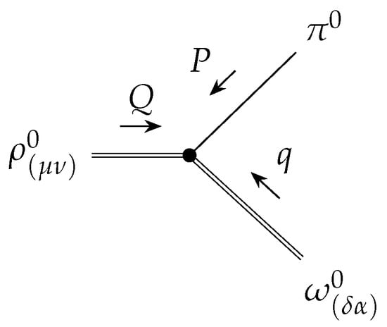
Figure 1. Convention of momentum and Lorentz index in the vertex ${\rho }^0{\omega }^0{\pi }^0$, where arrows indicate the direction of annihilation.

${\rho }^0{\omega }^0{\pi }^0$ On-Shell Vertex

The decay ${\rho }^0\to {\pi }^0{\pi }^0\gamma$ can be described within the $R\chi T$ framework, but its evaluation is hindered by its dependence on a set of LECs that remain unknown. Nonetheless, the number of independent couplings can be significantly reduced by employing on-shell vertices [11]. An on-shell vertex scenario corresponds to applying the Feynman rule for a vertex under the assumption that all external particles are on-shell, even when, in the Feynman amplitude, one of the legs corresponds to a virtual (off-shell) particle.

To define the on-shell vertex, we consider the process ${\rho }^0\left(Q\right)\to {\omega }^0\left(q\right){\pi }^0\left(P\right)$, where all the particles are on-shell and their corresponding momentum satisfy

$$\begin{array}{cc}\hfill Q^2=& m_{\rho }^2,\hfill \end{array}$$

(65)

$$\begin{array}{cc}\hfill q^2=& m_{\omega }^2,\hfill \end{array}$$

(66)

$$\begin{array}{cc}\hfill P^2=& m_{\pi }^2.\hfill \end{array}$$

(67)

We use the FeynCalc package [26,27] for tensor manipulations, which enables the reduction of the Feynman amplitude to

$${\mathcal{M}}_{\rho \to \omega \pi }=g_{\rho \omega \pi }{ϵ}_{\mu \nu \alpha \beta }{\displaystyle \frac{2Q^{\nu }{ϵ}_{\rho }^{\beta }}{m_{\rho }}}{\displaystyle \frac{2q^{\mu }{ϵ}_{\omega }^{\alpha }}{m_{\omega }}},$$

(68)

where ${ϵ}_{\rho }$ and ${ϵ}_{\omega }$ are the polarization vector of the $\rho$ and $\omega$ mesons, respectively. From the last expression, the on-shell Feynman rule for the $\rho \text{-}\omega \text{-}\pi$ vertex is given by

$$V_{\rho \omega {\pi }_{on-shell}}^{\mu \nu \delta \alpha }=g_{\rho \omega \pi }{ϵ}^{\delta \mu \alpha \nu },$$

(69)

where

$$g_{\rho \omega \pi }={\displaystyle \frac{m_{\pi }^2\left(d_1+8d_2\right)+d_3\left(m_{\rho }^2+m_{\omega }^2-m_{\pi }^2\right)}{F}}.$$

(70)

The tensor indices are assigned according to Figure 1. As shown, the on-shell vertex derived depends on a specific combination of LECs, whose values, according to Section 2, are well known.

3.2. Interaction Vertex Among the ${\omega }^0$, ${\gamma }^0$, and ${\pi }^0$ Particles

In this section, we closely follow the treatment presented in Section 3.1. The interaction vertex involving the $\omega ,\pi ,\gamma$ particles is derived from the Lagrangian given in Equation (26), taking into account only the relevant degrees of freedom and neglecting higher-order terms. The expressions thus derived are

$$\begin{array}{cc}\hfill V^{\mu \nu }& ={\displaystyle \frac{{\omega }^{\mu \nu }}{\sqrt{2}}}diag(1,1,0),\hfill \end{array}$$

(71)

$$\begin{array}{cc}\hfill {\overline{F}}^{\delta \alpha }& \equiv {\partial }^{\delta }{A}^{\alpha }-{\partial }^{\alpha }{A}^{\delta },\hfill \end{array}$$

(72)

$$\begin{array}{cc}\hfill {\mathcal{F}}_{+}^{\delta \alpha }& ={\displaystyle \frac{2}{3}}e{\overline{F}}^{\delta \alpha }diag(2,-1,-1),\hfill \end{array}$$

(73)

$$\begin{array}{cc}\hfill {\mathcal{F}}_{-}^{\delta \alpha }& =0,\hfill \end{array}$$

(74)

$$\begin{array}{cc}\hfill {\nabla }_{\alpha }{V}^{\mu \nu }& ={\displaystyle \frac{{\partial }_{\alpha }{\omega }^{\mu \nu }}{\sqrt{2}}}diag(1,1,0),\hfill \end{array}$$

(75)

$$\begin{array}{cc}\hfill {\chi }_{+}& =2m_{\pi }^{2}diag(1,1,-1).\hfill \end{array}$$

(76)

Consequently, the VJP operators in Equations (31)–(37) in terms of fields take the form

$$\begin{array}{cc}\hfill {\tilde{\mathcal{O}}}_{\omega \gamma \pi }^1& =-{\displaystyle \frac{2\sqrt{2}e}{F}}{ϵ}_{\mu \nu \delta \sigma }{\overline{F}}^{\delta \alpha }{\omega }^{\mu \nu }{\partial }_{\alpha }{\partial }^{\sigma }\pi ,\hfill \end{array}$$

(77)

$$\begin{array}{cc}\hfill {\tilde{\mathcal{O}}}_{\omega \gamma \pi }^2& =-{\displaystyle \frac{2\sqrt{2}e}{F}}{ϵ}_{\mu \nu \delta \sigma }{\overline{F}}^{\delta \sigma }{\omega }^{\mu \alpha }{\partial }_{\alpha }{\partial }^{\nu }\pi ,\hfill \end{array}$$

(78)

$$\begin{array}{cc}\hfill {\tilde{\mathcal{O}}}_{\omega \gamma \pi }^3& ={\displaystyle \frac{4\sqrt{2}e{m}_{\pi }^2}{F}}{ϵ}_{\mu \nu \delta \sigma }{\overline{F}}^{\delta \sigma }{\omega }^{\mu \nu }\pi ,\hfill \end{array}$$

(79)

$$\begin{array}{cc}\hfill {\tilde{\mathcal{O}}}_{\omega \gamma \pi }^4& =0,\hfill \end{array}$$

(80)

$$\begin{array}{cc}\hfill {\tilde{\mathcal{O}}}_{\omega \gamma \pi }^5& =-{\displaystyle \frac{2\sqrt{2}e}{F}}{ϵ}_{\mu \nu \delta \sigma }{\overline{F}}^{\delta \alpha }{\partial }_{\alpha }{\omega }^{\mu \nu }{\partial }^{\sigma }\pi ,\hfill \end{array}$$

(81)

$$\begin{array}{cc}\hfill {\tilde{\mathcal{O}}}_{\omega \gamma \pi }^6& =-{\displaystyle \frac{2\sqrt{2}e}{F}}{ϵ}_{\mu \nu \delta \sigma }{\overline{F}}^{\delta \sigma }{\partial }_{\alpha }{\omega }^{\mu \alpha }{\partial }^{\nu }\pi ,\hfill \end{array}$$

(82)

$$\begin{array}{cc}\hfill {\tilde{\mathcal{O}}}_{\omega \gamma \pi }^7& =-{\displaystyle \frac{2\sqrt{2}e}{F}}{ϵ}_{\mu \nu \delta \sigma }{\overline{F}}^{\delta \alpha }{\partial }^{\sigma }{\omega }^{\mu \nu }{\partial }_{\alpha }\pi .\hfill \end{array}$$

(83)

Therefore, the Feynman rule for the vertex ${\omega }^0{\pi }^0\gamma$, shown in Figure 2, is written as

$$V_{\omega \gamma \pi }^{\mu \nu l}=\sum _{a=1}^7{\displaystyle \frac{c_j}{M_V}}{\mathcal{V}}_{j\omega \pi \gamma }^{\mu \nu l},$$

(84)

where

$$\begin{array}{cc}\hfill {\mathcal{V}}_{1\omega \gamma \pi }^{\mu \nu l}& ={\displaystyle \frac{2\sqrt{2}ei}{F}}({ϵ}^{\mu \nu l\lambda }{k}_{\alpha }{P}^{\alpha }-{ϵ}^{\mu \nu \alpha \lambda }{k}_{\alpha }{P}^l)P_{\lambda },\hfill \end{array}$$

(85)

$$\begin{array}{cc}\hfill {\mathcal{V}}_{2\omega \gamma \pi }^{\mu \nu l}& ={\displaystyle \frac{4\sqrt{2}ei}{F}}{ϵ}^{\mu \delta \lambda l}{k}_{\delta }{P}_{\lambda }{P}^{\nu },\hfill \end{array}$$

(86)

$$\begin{array}{cc}\hfill {\mathcal{V}}_{3\omega \gamma \pi }^{\mu \nu l}& ={\displaystyle \frac{8\sqrt{2}ei{m}_{\pi }^2}{F}}{ϵ}^{\mu \nu l\lambda }{k}_{\lambda },\hfill \end{array}$$

(87)

$$\begin{array}{cc}\hfill {\mathcal{V}}_{4\omega \gamma \pi }^{\mu \nu l}& =0,\hfill \end{array}$$

(88)

$$\begin{array}{cc}\hfill {\mathcal{V}}_{5\omega \gamma \pi }^{\mu \nu l}& ={\displaystyle \frac{2\sqrt{2}ei}{F}}({ϵ}^{\mu \nu l\lambda }{k}_{\alpha }{q}^{\alpha }-{ϵ}^{\mu \nu \alpha \lambda }{k}_{\alpha }{q}^l)P_{\lambda },\hfill \end{array}$$

(89)

$$\begin{array}{cc}\hfill {\mathcal{V}}_{6\omega \gamma \pi }^{\mu \nu l}& ={\displaystyle \frac{4\sqrt{2}ei}{F}}{ϵ}^{\mu \lambda l\alpha }{k}_{\alpha }{q}^{\nu }{P}_{\lambda },\hfill \end{array}$$

(90)

$$\begin{array}{cc}\hfill {\mathcal{V}}_{7\omega \gamma \pi }^{\mu \nu l}& ={\displaystyle \frac{2\sqrt{2}ei}{F}}({ϵ}^{\mu \nu l\lambda }{k}_{\alpha }{P}^{\alpha }-{ϵ}^{\mu \nu \alpha \lambda }{k}_{\alpha }{P}^l)q_{\lambda }.\hfill \end{array}$$

(91)

The Lorentz indices $\mu ,\nu$ and l are assigned according to Figure 2.

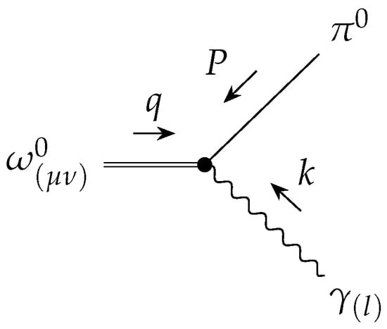
Figure 2. Convention of momentum and Lorentz index for the ${\omega }^0$, $\gamma$ and ${\pi }^0$ vertex, where arrows indicate the direction of annihilation.

${\omega }^0\gamma {\pi }^0$ On-Shell Vertex

Considering the ${\omega }^0\to {\pi }^0\gamma$ process, the Feynman amplitude, provided in Ref. [8], is given by

$${\mathcal{M}}_{{\omega }^0\to {\pi }^0\gamma }=e{g}_{\omega \pi }{ϵ}_{\alpha \beta \rho \sigma }{k}^{\sigma }{\displaystyle \frac{2{ϵ}_{\omega }^{\alpha }{q}^{\rho }}{m_{\omega }}}{ϵ}_{\gamma }^{\beta },$$

(92)

where $g_{\omega \pi }$ can be reduced, after using Equations (38)–(40), as follows,

$$g_{\omega \pi }={\displaystyle \frac{N_c}{32{\pi }^2{F}_{V}F}}{m}_{\omega }^2.$$

(93)

Therefore, the on-shell vertex is given by

$$V_{\omega \gamma \pi onshell}^{\mu \nu l}=e{g}_{\omega \pi }{ϵ}_{\mu l\nu \sigma }{k}^{\sigma },$$

(94)

which corresponds to the expression reported in [11].

3.3. ${\rho }^0$ Decay into ${\pi }^0{\pi }^0\gamma$

In this section, we analyze the process ${\rho }^0\to {\pi }^0{\pi }^0\gamma$ using the interaction Lagrangian given in Equation (47). At lowest order, the Feynman amplitude requires a $VJP$ and a $VVP$ vertex, with the $\omega$ treated as a virtual particle, as shown in Figure 3. It is found that the $\mathcal{BR}({\rho }^0\to {\pi }^0{\pi }^0\gamma )$ depends on the specific combination of LECs $c_{57}\equiv c_5+c_7$ and $d_4$. In order to reduce the number of unknown couplings, one can use the $\rho \omega \pi$ on-shell vertex, the $\omega \pi \gamma$ on-shell vertex or considering both vertices on shell.

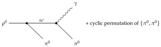
Figure 3. Lowest-order Feynman diagram for the process ${\rho }^0\left(Q\right)\to {\pi }^0\left(P_1\right){\pi }^0\left(P_2\right)\gamma \left(k\right)$, proceeding through a virtual $\omega$ resonance.

• Scenario 1: The decay ${\rho }^0\to {\pi }^0{\pi }^0\gamma$ via purely on-shell vertices.

First we calculate the branching ratio using both vertices on-shell, which are given in Equations (69) and (94). The corresponding Feynman amplitude is given by

$$\mathcal{M}={\left.\mathcal{M}\right|}_{q=P_1+k}+{\left.\mathcal{M}\right|}_{q=P_2+k}$$

(95)

where

$${\left.\mathcal{M}\right|}_q={\displaystyle \frac{8e{g}_{\rho }{g}_{\omega \pi \rho }}{m_{\rho }(M_V^2-q^2)M_V^2}}\left[\left({ϵ}_{\gamma }·{ϵ}_{\rho }\right)f_1+\left({ϵ}_{\rho }·k\right)\left({ϵ}_{\gamma }·f_2\right)+\left({ϵ}_{\rho }·q\right)\left({ϵ}_{\gamma }·f_3\right)\right],$$

(96)

and

$$\begin{array}{cc}\hfill f_1& =\left(k·q\right)\left(q·Q\right)-M_V^2\left(k·Q\right),\hfill \end{array}$$

(97)

$$\begin{array}{cc}\hfill f_2^{\alpha }& =M_V^2{Q}^{\alpha }-q^{\alpha }\left(q·Q\right),\hfill \end{array}$$

(98)

$$\begin{array}{cc}\hfill f_3^{\alpha }& =q^{\alpha }\left(k·Q\right)-Q^{\alpha }\left(k·q\right).\hfill \end{array}$$

(99)

The scalar products, expressed in terms of the Mandelstam variables, defined as $m_{31}\equiv {(k+P_1)}^2$, $m_{23}\equiv {(k+P_2)}^2$, and $m_{12}\equiv {(P_1+P_2)}^2$, are written as follows:

$$\begin{array}{cc}\hfill Q·P_1& ={\displaystyle \frac{m_{\rho }^2+m_{\pi }^2-m_{23}}{2}},\hfill \end{array}$$

(100)

$$\begin{array}{cc}\hfill Q·k& ={\displaystyle \frac{m_{\rho }^2-m_{12}}{2}},\hfill \end{array}$$

(101)

$$\begin{array}{cc}\hfill Q·P_2& ={\displaystyle \frac{m_{\rho }^2+m_{\pi }^2-m_{31}}{2}},\hfill \end{array}$$

(102)

$$\begin{array}{cc}\hfill k·P_2& ={\displaystyle \frac{m_{23}-m_{\pi }^2}{2}},\hfill \end{array}$$

(103)

$$\begin{array}{cc}\hfill P_1·P_2& ={\displaystyle \frac{m_{12}-2m_{\pi }^2}{2}}.\hfill \end{array}$$

(104)

The kinematics of a three-body decay can be described by only two independent variables. In this work, we chose $m_{12}$ and $m_{23}$; therefore, the branching ratio is calculated as

$$\mathcal{BR}({\rho }^0\to {\pi }^0{\pi }^0\gamma )={\displaystyle \frac{1}{{\mathrm{\Gamma }}_{\rho }}}{\displaystyle \frac{1}{{\left(2\pi \right)}^3}}{\displaystyle \frac{1}{32m_{\rho }^3}}{\int }_{m_{\pi }^2}^{{(m_{\rho }-m_{\pi })}^2}{\int }_{m_{{23}_{-}}}^{m_{{23}_{+}}}Xd{m}_{12}d{m}_{23},$$

(105)

where

$$X={\displaystyle \frac{1}{3}}\sum _{r=1}^3\sum _{s=1}^2\mid \mathcal{M}{\mid }^2,$$

(106)

and ${\mathrm{\Gamma }}_{\rho }$ denotes the total decay width. The minimum and maximum values of $m_{12}$ and $m_{23}$ define the boundaries of the region known as the Dalitz plot (Figure 4), which are determined by the following relations:

$$\begin{array}{cc}\hfill m_{23\pm }& ={\left(E_2^{\ast }+E_3^{\ast }\right)}^2-{\left(E_2^{\ast }\mp \sqrt{E_3^{\ast 2}-m_{\pi }^2}\right)}^2,\hfill \end{array}$$

(107)

$$\begin{array}{cc}\hfill E_2^{\ast }& ={\displaystyle \frac{m_{12}-m_{\pi }^2}{2\sqrt{m_{12}}}},\hfill \end{array}$$

(108)

$$\begin{array}{cc}\hfill E_3^{\ast }& ={\displaystyle \frac{m_{\rho }^2-m_{12}-m_{\pi }^2}{2\sqrt{m_{12}}}}.\hfill \end{array}$$

(109)

The values of the meson masses and decay widths, according to the Particle Data Group [3], are $m_{\omega }=782.66\left(13\right)\mathrm{MeV}$, $m_{\rho }=775.26\left(23\right)\mathrm{MeV}$, $m_{\pi }=134.9768\left(5\right)\mathrm{MeV}$, ${\mathrm{\Gamma }}_{\rho }=147.4\left(8\right)\mathrm{MeV}$ and ${\mathrm{\Gamma }}_{\omega }=8.68\left(13\right)\mathrm{MeV}$, where the numbers in parentheses indicate the uncertainties. Additionally, we take from Ref. [8] the values $M_V=m_{\rho }$, $F_V=92.4\mathrm{MeV}$, and $N_c=3$.

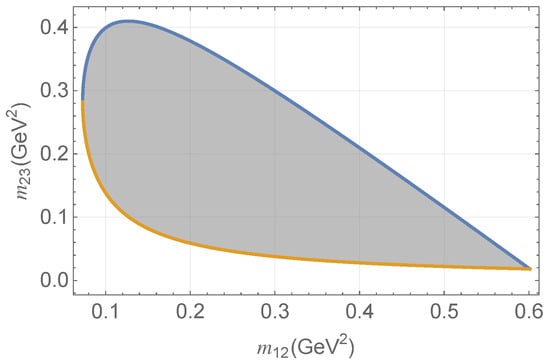
Figure 4. Kinematically allowed region (Dalitz plot) bounded by the blue and orange curves for the decay ${\rho }^0\to {\pi }^0{\pi }^0\gamma$. The blue and orange lines indicate the upper and lower kinematic limits, respectively, given by Equation (107).

The prediction with both vertices on-shell, using the relations (41)–(43), gives the value

$$\mathcal{BR}{({\rho }^0\to {\pi }^0{\pi }^0\gamma )}_{onshell}=2.111\left(10\right)\times {10}^{-4},$$

(110)

while using Equations (44)–(46) yields

$$\mathcal{BR}{({\rho }^0\to {\pi }^0{\pi }^0\gamma )}_{onshell}=1.606\left(6\right)\times {10}^{-4}.$$

(111)

The propagated error reported in Equations (111) and (110) has been estimated as follows. The inputs parameters reported by the PDG have an uncertainty $\sigma$; thus, the evaluation is performed using the central value of all inputs, as well as the central value plus $1\sigma$ and minus $1\sigma$. Finally, the uncertainty is collected as the sum of the deviations from the central value.

Comparing our prediction with the experimental value $\mathcal{BR}({\rho }^0\to {\pi }^0{\pi }^0\gamma )=4.5\left(8\right)\times {10}^{-5}$ clearly shows that taking both vertices on-shell is not consistent.

• Scenario 2: The decay ${\rho }^0\to {\pi }^0{\pi }^0\gamma$ via the on-shell $V_{\rho \omega \pi }$ vertex.

In this section we treat the vertex $V_{\omega \gamma \pi }$ (85)–(91) as off-shell, whereas the $V_{\rho \omega \pi }$ vertex remains on-shell (69). The corresponding Feynman amplitude for the ${\rho }^0\to {\pi }^0{\pi }^0\gamma$ decay is then given by

$$\mathcal{M}={\displaystyle \frac{16i\sqrt{2}e{g}_{\rho \omega \pi }}{F{m}_{\rho }{M}_V^2}}\left[-c_{57}{H}_1+{\displaystyle \frac{c_{56}{M}_V^2{H}_2-c_{13}{m}_{{\pi }^2}{H}_3+c_{125}{H}_4}{M_V^2-{\left(k+P_2\right)}^2}}\right]+\{P_1⟷P_2\},$$

(112)

where the functions $H_1,H_2,H_3$, and $H_4$ are given in Appendix A. For simplicity, we defined the following notation

$$\begin{array}{cc}\hfill c_1+4c_3& \equiv c_{13},\hfill \end{array}$$

(113)

$$\begin{array}{cc}\hfill c_1-c_2+c_5& \equiv c_{125},\hfill \end{array}$$

(114)

$$\begin{array}{cc}\hfill c_5-c_6& \equiv c_{56},\hfill \end{array}$$

(115)

$$\begin{array}{cc}\hfill c_5+c_7& \equiv c_{57}.\hfill \end{array}$$

(116)

When the relations (38)–(40) are applied, the Equation (112) depend exclusively on $c_{57}$. Assuming that the theoretical prediction matches the experimental branching ratio, one obtains a quadratic expression in $c_{57}$. Using the constraints (43), we find the roots $c_{57}=\{0.032\left(3\right),-0.025\left(3\right)\}$. Similarly, applying the constraints (46) yields the solutions $c_{57}=\{0.030\left(3\right),-0.025\left(3\right)\}$.

• Scenario 3: The decay ${\rho }^0\to {\pi }^0{\pi }^0\gamma$ via the on-shell $V_{\omega \gamma \pi }$ vertex.

Here, we take the $V_{\omega \gamma \pi }$ vertex (94) to be on-shell, whereas the $V_{\rho \omega \pi }$ vertex (61)–(64) is kept off-shell. Consequently, the Feynman amplitude simplifies to

$$\begin{array}{cc}\hfill \mathcal{M}& ={\displaystyle \frac{8e{g}_{\omega \pi }}{F{m}_{\rho }{M}_V^2}}\left[d_4{h}_1+{\displaystyle \frac{-d_{12}{m}_{\pi }^2{h}_2+d_3{h}_3}{M_V^2-{(k+P_2)}^2}}\right]+\{P_1⟷P_2\},\hfill \end{array}$$

(117)

where, for simplicity, it was defined the relation

$$d_1+8d_2\equiv d_{12},$$

(118)

and the functions $h_1$, $h_2$, and $h_3$ are defined in the Appendix A.

When the relations (41) and (42)—or, alternatively, (44) and (45)—are applied, Equation (117) simplifies and the BR becomes a quadratic function of $d_4$. Analogous to the analysis performed in the previous scenario, the solutions are $d_4=\{0.901\left(54\right),-0.221\left(54\right)\}$ using the constraints (41)–(43) and $d_4=\{1.059\left(65\right),-0.327\left(65\right)\}$ using the constraints (44)–(46). A similar analysis was carried out in Ref. [11] for the decay $\omega \to {\pi }^0{\pi }^0\gamma$, and our central values are in reasonable agreement with their results, $d_4=\{0.82\left(5\right),-0.12\left(5\right)\}$.

• Scenario 4: The decay ${\rho }^0\to {\pi }^0{\pi }^0\gamma$ with off-shell vertices.

Finally, we consider the scenario in which both vertices are off-shell. In this case, the corresponding Feynman amplitude is given by

$$\begin{array}{c}\hfill \mathcal{M}={\displaystyle \frac{16ie\sqrt{2}}{F^2{m}_{\rho }{M}_V^3}}\left[{\displaystyle \frac{c_{56}{M}_V^2{l}_1+c_{13}{m}_{\pi }^2{l}_2-c_{57}{l}_3-c_{125}{l}_4}{M_V^2-{\left(k+P_2\right)}^2}}\right]+P_1⟷P_2.\end{array}$$

(119)

By applying the large-${\mathrm{N}}_{\mathrm{c}}$ constraints discussed in Section 2, Equation (119) is found to depend only on $c_{57}$ and $d_4$. The dependence on $d_4$ is contained within the functions $l_1,l_2,l_3$, and $l_4$, which are defined in the Appendix A.

Prior to deriving the solution for $c_{57}$ and $d_4$ in this scenario, we analyze the impact of using the value of $c_{57}$ obtained in scenarios 2 together with the value of $d_4$ from scenario 3. The results of this combination are presented in Table 1.

Table 1. The prediction for $\mathcal{BR}\equiv \mathcal{BR}({\rho }^0\to {\pi }^0{\pi }^0\gamma )$ computed using a combination of the values of $c_{57}$ and $d_4$ from scenarios 2 and 3.

Constraints (38)–(43)			Constraints (44)–(46)
$c_{57}$	$d_4$	$\mathcal{BR}\times {10}^{-5}$	$c_{57}$	$d_4$	$\mathcal{BR}\times {10}^{-5}$
0.032(3)	0.901(54)	$3.08\left(63\right)$	0.030(3)	1.059(65)	$3.65\left(88\right)$
−0.025(3)	0.901(54)	$1.17\left(35\right)$	−0.025(3)	1.059(65)	$1.74\left(53\right)$
0.032(3)	−0.221(54)	$0.63\left(19\right)$	0.030(3)	−0.327(65)	$0.93\left(30\right)$
−0.025(3)	−0.221(54)	$0.78\left(20\right)$	−0.025(3)	−0.327(65)	$1.09\left(30\right)$

The results presented in Table 1 indicate that the combination of on-shell and off-shell vertices provides a more accurate estimation of the branching ratio compared to the scenario that employs solely on-shell vertices. For instance, the parameter pair $(c_{57},d_4)=(0.030\left(3\right),1.059\left(65\right))$ yields a $\mathcal{BR}({\rho }^0\to {\pi }^0{\pi }^0\gamma )=3.65\left(88\right)\times {10}^{-5}$, representing a notable improvement with respect to the result obtained in scenario 1. However, this value remains below the experimental measurement, $\mathcal{BR}({\rho }^0\to {\pi }^0{\pi }^0\gamma )=4.5\left(8\right)\times {10}^{-5}$, corresponding to a relative deviation of approximately $19\%$ with respect to the central value. However, the procedure used to construct the data in Table 1 is not fully consistent. Consequently, the most effective approach appears to be the use of purely off-shell vertices. Within this framework, a numerical contour solution in the $(c_{57},d_4)$ parameter space can be derived, as shown in Figure 5, which identifies the region consistent with the experimental branching ratio.

Figure 5. Geometric locus in the ($c_{57},d_4$) parameter space that matches the experimental $\mathcal{BR}(\rho \to {\pi }^0{\pi }^0\gamma )=4.5\times {10}^{-5}$, under the constraints (38)–(43).

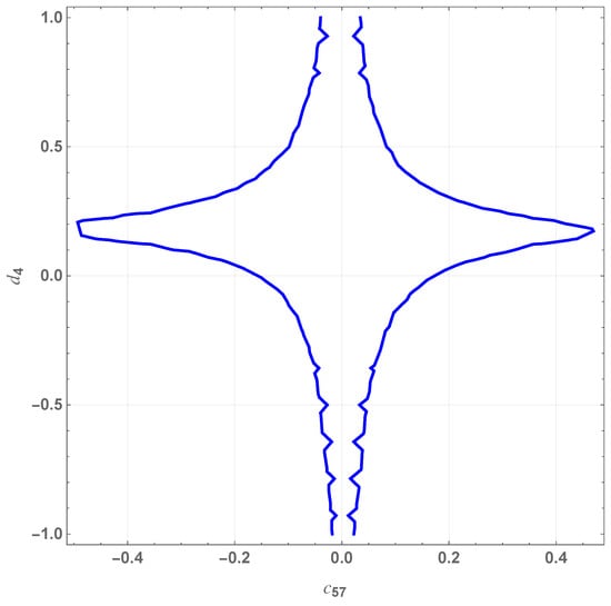
Selected values from this solution are listed in Table 2.

Table 2. In the first column, the value of $d_4$ is selected, while the two solutions shown in the second and third columns are obtained by applying the constraints (38)–(43), assuming that the theoretical prediction matches the experimental BR.

${\mathit{d}}_4$	${\mathit{c}}_{57}\left(\mathit{sol}1\right)$	${\mathit{c}}_{57}\left(\mathit{sol}2\right)$
−0.98	0.03	−0.03
0.90	0.03	−0.03
−0.80	0.03	−0.03
−0.70	0.04	−0.03
−0.60	0.04	−0.04
−0.50	0.05	−0.04
−0.40	0.06	−0.05
−0.30	0.07	−0.06
−0.20	0.09	−0.08
−0.10	0.12	−0.10
0.02	0.20	−0.18
0.10	0.33	−0.31
0.20	0.44	−0.53
0.30	0.21	−0.25
0.40	0.12	−0.15
0.50	0.09	−0.10
0.60	0.07	−0.08
0.70	0.05	−0.07
0.80	0.05	−0.05
0.90	0.04	−0.05
0.98	0.04	−0.04

It is worth noting that the pairs $(c_{57},d_4)$ in Figure 5 exhibit three predominant features in the differential branching ratio $dB/d\sqrt{m_{12}}\equiv d\mathcal{BR}(\rho \to {\pi }^0{\pi }^0\gamma )/d\sqrt{m_{12}}$, as illustrated in Figure 6. The blue curve appears to qualitatively agree with the results reported in Ref. [20], where the interaction is mediated by pion loops within a framework that combines the Vector Meson Dominance model and the linear sigma model.

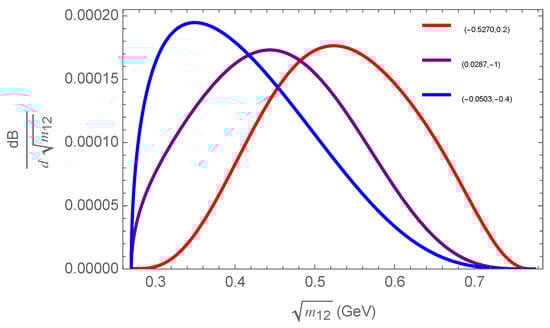
Figure 6. In this plot, we show the $dB/d\sqrt{m_{12}}$ using three specific pairs $(c_{57},d_4)$ from Figure 5.

4. Conclusions

In this work, we have studied the decay process ${\rho }^0\to {\pi }^0{\pi }^0\gamma$ within the framework of chiral perturbation theory with resonances. Our analysis shows that the Branching Ratio (BR) depends exclusively on the low-energy couplings $c_{57}$ and $d_4$. To address this, we analyzed all possible scenarios arising from different combinations of on-shell and off-shell interaction vertices. Our results indicate that the purely on-shell scenario yields a value significantly below the experimental branching ratio, suggesting that this scenario does not provide a reliable description of the process. On the other hand, scenarios in which one of the vertices is taken on-shell reduce the number of unknown couplings, thereby enabling the determination of the remaining couplings from the roots of a quadratic equation. It is worth noting that this approach does not allow us to discriminate between the two roots. Pursuing this line of reasoning, we use both couplings simultaneously and find that, even in the best-case scenario, the theoretical prediction differs by 19% from the experimental value of $4.5\times {10}^{-5}$ (Table 1). This discrepancy suggests that the vertices must be off-shell. Our results are presented as a region of possible values for $c_{57}$ and $d_4$, consistent with the experimental BR, as shown in Figure 5. Considering the result $d_4=\{0.82\left(5\right),-0.12\left(5\right)\}$ reported in Ref. [11], obtained through the decay $\omega \to {\pi }^0{\pi }^0\gamma$, we obtain the values $c_{57}=\{0.04,-0.05\}$ for $d_4=0.82$ and $c_{57}=\{0.11,-0.10\}$ for $d_4=-0.12$. However, these values do not fall within the estimate $\left|c_i\right|\le 0.015$ of Ref. [9]. It must be emphasized that the value of $d_4$ obtained in Ref. [11] assumes the $\rho \omega \pi$ vertex to be on-shell, whereas the estimate for $c_i$ in Ref. [9] is based on an informed estimate inferred from the behaviour of the remaining couplings. Consequently, these estimates must therefore be interpreted with caution. In addition, we provide the differential branching ratio (dBR), which depends on the precise values of the LECs. In particular, Figure 6 shows the dBR for three representative sets of $(c_{57},d_4)$, where the shape of the distribution can be clearly observed. This information can be used to further constrain the parameter space (work in progress) by fitting to the experimental dBR data.

References

- Schwartz, M.D. Quantum Field Theory and the Standard Model; Cambridge University Press: Cambridge, UK, 2014. [Google Scholar]
- Grossman, Y.; Nir, Y. The Standard Model: From Fundamental Symmetries to Experimental Tests; Princeton University Press: Princeton, NJ, USA, 2023. [Google Scholar]
- Navas, S.; Amsler, C.; Gutsche, T.; Hanhart, C.; Hernández-Rey, J.J.; Lourenço, C.; Masoni, A.; Mikhasenko, M.; Mitchell, R.E.; Patrignani, C.; et al. Review of particle physics. Phys. Rev. D 2024, 110, 030001. [Google Scholar] [CrossRef]
- Weinberg, S. Phenomenological Lagrangians. Phys. A Stat. Mech. Its Appl. 1979, 96, 327–340. [Google Scholar] [CrossRef]
- Scherer, S.; Schindler, M. A Primer for Chiral Perturbation Theory; Lecture Notes in Physics; Springer: Berlin/Heidelberg, Germany, 2011. [Google Scholar] [CrossRef]
- Pich, A. Chiral perturbation theory. Rep. Prog. Phys. 1995, 58, 563. [Google Scholar] [CrossRef]
- Ecker, G.; Gasser, J.; Pich, A.; De Rafael, E. The role of resonances in chiral perturbation theory. Nucl. Phys. B 1989, 321, 311–342. [Google Scholar] [CrossRef]
- Ruiz-Femenía, P.D.; Pich, A.; Portolés, J. Odd-intrinsic-parity processes within the resonance effective theory of QCD. J. High Energy Phys. 2003, 003. [Google Scholar] [CrossRef]
- Miranda, J.A.; Roig, P. New τ-based evaluation of the hadronic contribution to the vacuum polarization piece of the muon anomalous magnetic moment. Phys. Rev. D 2020, 102, 114017. [Google Scholar] [CrossRef]
- Aliberti, R.; Aoyama, T.; Balzani, E.; Bashir, A.; Benton, G.; Bijnens, J.; Biloshytskyi, V.; Blum, T.; Boito, D.; Bruno, M.; et al. The anomalous magnetic moment of the muon in the Standard Model: An update. Phys. Rept. 2025, 1143, 1–158. [Google Scholar] [CrossRef]
- Chen, C.; Duan, C.G.; Guo, Z.H. Triple-product asymmetry in the radiative two-pion tau decay. J. High Energy Phys. 2022, 2022, 144. [Google Scholar] [CrossRef]
- Ecker, G.; Gasser, J.; Leutwyler, H.; Pich, A.; De Rafael, E. Chiral Lagrangians for massive spin-1 fields. Phys. Lett. B 1989, 223, 425–432. [Google Scholar] [CrossRef]
- Roig, P.; Cillero, J.J.S. Consistent high-energy constraints in the anomalous QCD sector. Phys. Lett. B 2014, 733, 158–163. [Google Scholar] [CrossRef]
- Kampf, K.; Novotný, J. Resonance saturation in the odd-intrinsic parity sector of low-energy QCD. Phys. Rev. D 2011, 84, 014036. [Google Scholar] [CrossRef]
- Cirigliano, V.; Ecker, G.; Eidemüller, M.; Kaiser, R.; Pich, A.; Portolés, J. Towards a consistent estimate of the chiral low-energy constants. Nucl. Phys. B 2006, 753, 139–177. [Google Scholar] [CrossRef]
- Gómez Dumm, D.; Roig, P. Resonance Chiral Lagrangian analysis of τ− → η(′)π−π0ντ. Phys. Rev. D 2012, 86, 076009. [Google Scholar] [CrossRef]
- Gómez Dumm, D.; Pich, A.; Portolés, J. πππντ decays in the resonance effective theory. Phys. Rev. D 2004, 69, 073002. [Google Scholar] [CrossRef]
- Cirigliano, V.; Ecker, G.; Eidemüller, M.; Pich, A.; Portolés, J. <VAP> Green function in the resonance region. Phys. Lett. B 2004, 596, 96–106. [Google Scholar] [CrossRef]
- Achasov, M.N.; Beloborodov, K.I.; Berdyugin, A.V.; Bogdanchikov, A.G.; Bozhenok, A.V.; Bukin, A.D.; Bukin, D.A.; Burdin, S.V.; Vasil’ev, A.V.; Ganyushin, D.I.; et al. The e+e− → π0π0γ process below 1.0 GeV. J. Exp. Theor. Phys. Lett. 2000, 71, 355–358. [Google Scholar] [CrossRef]
- Bramon, A.; Escribano, R.; Lucio M, J.L.; Napsuciale, M. Scalar σ meson effects in ρ and ω decays into π0π0γ. Phys. Lett. B 2001, 517, 345–354. [Google Scholar] [CrossRef]
- Achasov, M.N.; Beloborodov, K.I.; Berdyugin, A.V.; Bogdanchikov, A.G.; Bozhenok, A.V.; Bukin, D.A.; Burdin, S.V.; Vasiljev, A.V.; Golubev, V.B.; Dimova, T.V.; et al. Experimental study of ρ → π0π0γ and ω → π0π0γ decays. Phys. Lett. B 2002, 537, 201–210. [Google Scholar] [CrossRef]
- Gokalp, A.; Yilmaz, O. The decay ρ0 → π0π0γ and the role of σ-meson. Phys. Lett. B 2001, 508, 25–30. [Google Scholar] [CrossRef]
- Marco, E.; Hirenzaki, S.; Oset, E.; Toki, H. Radiative decay of ρ0 and φ mesons in a chiral unitary approach. Phys. Lett. B 1999, 470, 20–26. [Google Scholar] [CrossRef]
- Gokalp, A.; Solmaz, S.; Yilmaz, O. Scalar σ meson effects in radiative ρ0-meson decays. Phys. Rev. D 2003, 67, 073007. [Google Scholar] [CrossRef]
- Akhmetshin, R.R.; Aulchenko, V.M.; Banzarov, V.S.; Baratt, A.; Barkov, L.M.; Baru, S.E.; Bashtovoy, N.S.; Bondar, A.E.; Bondarev, D.V.; Bragin, V.A.; et al. Study of the process e+e− → π0π0γ in c.m. energy range 600–970 MeV at CMD-2. Phys. Lett. B 2004, 580, 119–128. [Google Scholar] [CrossRef]
- Shtabovenko, V.; Mertig, R.; Orellana, F. FeynCalc 10: Do multiloop integrals dream of computer codes? Comput. Phys. Commun. 2025, 306, 109357. [Google Scholar] [CrossRef]
- Mertig, R.; Böhm, M.; Denner, A. FeynCalc—Computer-algebraic calculation of Feynman amplitudes. Comput. Phys. Commun. 1991, 64, 345–359. [Google Scholar] [CrossRef]
Disclaimer/Publisher’s Note: The statements, opinions and data contained in all publications are solely those of the individual author(s) and contributor(s) and not of MDPI and/or the editor(s). MDPI and/or the editor(s) disclaim responsibility for any injury to people or property resulting from any ideas, methods, instructions or products referred to in the content. |
© 2025 by the authors. Licensee MDPI, Basel, Switzerland. This article is an open access article distributed under the terms and conditions of the Creative Commons Attribution (CC BY) license (https://creativecommons.org/licenses/by/4.0/).