Abstract
Sensor-rich Automated Guided Vehicles (AGVs) are increasingly deployed in logistics, yet large fleets relying on fixed tracks face high maintenance costs and frequent route conflicts. This study targets rail-based material handling and proposes an end-to-end multi-AGV navigation pipeline under realistic operational constraints. A conflict-aware global planner, extended from the A* algorithm, generates feasible routes, while a multi-sensor perception stack integrates LiDAR and camera data to distinguish moving AGVs, static obstacles, and task targets. Based on this perception, a Deep Q-Network (DQN) policy with a tailored reward function enables real-time dynamic obstacle avoidance in complex traffic. Simulation results demonstrate that, compared with the Artificial Potential Field (APF) baseline, the proposed GG-DRL approach reduces collisions by ~70%, lowers planning time by 25–30%, shortens paths by 10–15%, and improves smoothness by 20–25%. On the Maze Benchmark Map, GG-DRL surpasses classical planners (e.g., RRT) and deep RL baselines (e.g., DDPG) in path quality, computation, and avoidance behavior, achieving an average path length of 81.12, computation time of 11.94 s, 5.2 avoidance maneuvers, and smoothness of 0.86. Robustness is maintained as a dynamic obstacles scale up to 30. These findings confirm that combining multi-sensor fusion with deep reinforcement learning enhances AGV safety, efficiency, and reliability, with broad potential for intelligent railway logistics.
1. Introduction
In recent years, with the advancement of technological innovation and automation technology, the transportation industry is shifting towards intelligence, informatization, and automation. The integration and development of rail transportation with artificial intelligence are becoming increasingly close. Rail transportation systems, with their advantages of high capacity, comfort, and eco-friendliness, are seeing a notably accelerated pace of construction [1]. To promote the application and development of intelligent and automation technologies in the rail transportation field, the use of Automated Guided Vehicles (AGVs) as tools for material transportation has become a hot topic in the industry. Meanwhile, AGVs are also seen as an indispensable part of the push towards intelligent development in the logistics industry, attracting widespread attention from researchers within the sector.
Against the backdrop of rapid developments in smart logistics and automated warehouse systems, the path planning for multiple Automated Guided Vehicle (AGV) systems has become a critical technological challenge for enhancing system efficiency and safety. Effective path planning must ensure collision-free navigation of AGVs in complex environments, while also seeking to improve planning efficiency and reduce the overall system’s energy consumption. To this end, scholars have proposed a series of studies based on traditional path planning algorithms to address the path planning issues in multi-AGV systems. Yang et al. explored a traffic control algorithm for multi-AGV path planning based on system-level scheduling, providing theoretical support and practical verification for the scheduling of multiple AGVs in dock transportation tasks [2]. Pratama et al. aimed to design an efficient multi-agent AGV path planning system based on an improved A* algorithm, effectively managing the path allocation among multiple AGVs to avoid collisions through centralized processing in a server [3]. Hu et al. further optimized the traditional A* algorithm by adding turn weight in the heuristic function and employing a task segmentation strategy, proposing an improved A* algorithm to enhance search efficiency and thoroughness in real working environments [4]. Tien & Nguyen introduced a dynamic path planning method based on updating the weight graph, effectively addressing the operational challenges of multi-AGV systems in medical environments [5].
Furthermore, Huang et al. enhanced the performance of the algorithm in obstacle avoidance and path smoothness by improving the genetic algorithm, effectively increasing the path planning efficiency of the original algorithm [6]. In the context of the growing development of smart vehicles and autonomous driving technologies, multi-sensor fusion technology has become an indispensable part of environmental perception and decision-making. By utilizing information from different sensors, sensor fusion technology can provide a more comprehensive and accurate understanding of the environment, thereby offering reliable decision support for smart vehicles.
In recent years, the application research of multi-sensor fusion in the field of intelligent vehicle environmental perception has gained widespread attention. Scholars have proposed various fusion strategies and frameworks to improve the accuracy and robustness of the perception system. Shi and others discussed methods to improve multi-sensor fusion effects through spatiotemporal evidence generation and independent visual channels, significantly enhancing the detection and classification accuracy of vehicle environmental perception. This research highlighted the potential and effectiveness of multi-sensor fusion in real traffic environments [7].
Senel and others proposed a modular, real-time multi-sensor fusion framework specifically for real-time multi-object tracking in intelligent transportation applications, showcasing the framework’s ability to continue operating even when individual sensors fail, highlighting the system’s adaptability and robustness [8]. Bouain focused on an embedded multi-sensor data fusion design for intelligent vehicle environmental perception tasks, based on a modular and scalable architecture, demonstrating the application potential of sensor fusion technology in resource-constrained environments [9].
Xiang and others reviewed multi-sensor fusion and collaborative perception research in the field of autonomous driving, proposing a new classification method for multi-sensor fusion. This research provides a new perspective for understanding and categorizing different fusion strategies, guiding future research directions [10]. Jayaratne explored a scalable fusion technique based on unsupervised machine learning to improve the environmental perception capabilities of autonomous robots in unknown environments [11].
With the rapid development of smart manufacturing and logistics automation technologies, the path planning problem for multiple Automated Guided Vehicles (AGV) has become one of the research hotspots. In complex environments, how to quickly and safely plan the optimal path for AGVs is not only related to the system’s operational efficiency but also directly affects the level of intelligence and automation of the entire smart system.
Deep reinforcement learning, as a machine learning method capable of acquiring optimal strategies through learning, has shown tremendous application potential and research value in the field of multi-AGV path planning. Liao and others [12] explored a reinforcement learning-based AGV path planning model that effectively guides AGVs to plan optimal paths in complex environments through the Sarsa algorithm combined with a simulated annealing strategy.
The proposed potential field method combined with the Deep Q-Network algorithm effectively addresses the shortcomings of traditional reinforcement learning algorithms in dealing with large-scale state spaces, significantly improving the success rate and efficiency of AGV path planning in warehousing logistics [12]. Yin and others proposed a curiosity-driven deep reinforcement learning method to solve the path planning problem of AGVs in real and complex environments. This method uses an enhanced Proximal Policy Optimization (PPO) method and provides additional intrinsic rewards for AGV agents in sparse reward scenarios through a curiosity mechanism, showing that AGVs can efficiently plan reasonable and safe paths [13].
Guo and others introduced an autonomous path planning method for AGVs based on deep reinforcement learning, using a Dueling Double Deep Q-Network with Prioritized Experience Replay (Dueling DDQN-PER) to learn AGV control in a simulated Intelligent Logistics System (ILS) environment, significantly improving the AGV’s target approach capability and obstacle avoidance ability [14]. Ye and others developed a multi-agent reinforcement learning algorithm for multiple AGVs aimed at minimizing overall energy consumption. This algorithm, based on the Multi-Agent Deep Deterministic Policy Gradient (MADDPG) algorithm, effectively addresses energy efficiency routing problems providing an effective solution for energy-efficient routing in complex environments [15]. Zhang and others targeted the dynamic path planning problem of AGVs in mixed-flow workshops. Based on reinforcement learning theory, they proposed an improved reinforcement learning algorithm. By designing heuristic reward functions and action selection strategies with harmony functions, they enhanced the effectiveness of AGV motion path exploration [16].
While researchers have achieved some results, there are still the following issues: Firstly, traditional graph-search-based path planning methods, when conducting a complete exploration of the environment, suffer from increased complexity and high computational costs due to the need to traverse all nodes in a directed graph. Moreover, most traditional graph-search-based path planning methods are mainly used for global searches in static environments and cannot meet the needs of dynamic planning scenarios in rail transport environments.
Additionally, some traditional path planning methods assume a known environment and do not consider real-world factors when defining multi-robot path planning problems, whereas AGVs in real applications gradually become aware of dynamic environmental information. Secondly, although multi-sensor fusion technology has been used in fields such as vision navigation [17], multi-robot dynamic planning [18], and autonomous driving [19], each multi-sensor fusion technology is based on specific use scenarios (such as obstacle avoidance technology designed for the living scenarios of visually impaired people) and cannot be applied to rail transport environments.
Furthermore, different mobile robots are equipped with different types of sensors, and there are significant differences in the processing algorithms for different types of sensors. This article uses AGVs equipped with LiDAR and camera sensors for rail transport environments. LiDAR [20] is not affected by external influences and can better adapt to complex dynamic environments with interference. Using vision sensors [21] can richly perceive environmental information, detect obstacles, and achieve obstacle avoidance. Lastly, most existing multi-agent planning algorithms represent agents with rectangular boxes or other simple shapes.
However, this article, based on the rail transport environment, needs to consider the practical application of algorithms. The rail transport material transportation environment is complex, requiring not only consideration of static obstacles but also dynamic obstacles (other AGVs besides oneself). In addition, existing DRL algorithms for path planning are only tailored for specific scenarios, showing inapplicability in the field of rail transportation.
Addressing the aforementioned issues, this paper focuses on rail transport material handling and primarily investigates multi-AGV path planning methods, which are divided into three main parts as shown in Figure 1. The first part of the research addresses the high time cost issues caused by collisions with obstacles during AGV cargo transportation in complex dynamic rail transport environments. It establishes multi-AGV path planning, combining the characteristics of the rail transport material transportation environment. Using the A* path algorithm as a baseline and integrating traditional path planning methods with deep learning approaches, it autonomously learns heuristic functions to minimize search costs in complex environments.
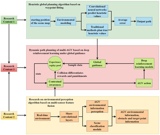
Figure 1.
Technical roadmap.
The method is trained by minimizing the squared error between the predicted values at each waypoint and the target cost values, ultimately fitting each AGV with an optimal path of minimum cumulative cost for global AGV path planning. Traditional AGVs that move along predetermined paths or carry out transportation tasks guided by wires require high maintenance costs for the lines, and AGV queues can cause time costs due to congestion.
To address these issues, the second part of the research utilizes the binocular cameras and LiDAR sensors carried by new AGV carts. By capturing the environmental features around the AGVs with sensors and using LSTM networks to extract LiDAR point cloud data and time-based AGV state information for obstacle perception, a twin deep convolutional neural network is employed.
Through shared convolutional layers, AGV environmental information perception modules and scene classification modules extract AGV camera information, obtaining classifications of different types of obstacles and targets. The LiDAR information and camera features are integrated with the cart’s own information to obtain a comprehensive environmental perception model. In the rail transport material handling environment, multiple AGVs work in parallel, carrying goods and serving as dynamic obstacles to each other, all within a large-scale AGV operating environment.
How to achieve collision-free transportation to the destination is very important. For the avoidance of dynamic obstacles (other AGVs, etc.) in a multi-AGV operating environment, the third part of the research proposes a study on multi-AGV dynamic path planning under global guidance based on deep reinforcement learning. Combining the deep reinforcement learning model with global guidance, a differentiated reward and punishment method for multi-AGV dynamic planning is trained: taking the multi-AGV paths output by the deep convolutional model in the first part as global guidance, real-time AGV feedback on motion and environmental information is obtained through the environmental perception model in the second part.
The relative positions of waypoints are used to determine short-term goals, and decisions are made using the deep reinforcement learning model, with corresponding rewards and punishments for AGV movements, and each decision-making state is stored in an experience replay pool as a training sample for future use. Different rewards and punishments are given to AGVs depending on the outcome of each navigation attempt. Utilizing the initial path obtained from traditional algorithms as a baseline to provide global guidance, the convergence speed of deep reinforcement learning is accelerated. Through the designed reward function, unmanned vehicles can roughly follow the initial path to quickly reach the target during navigation, with a smoother trajectory and higher navigation efficiency.
2. Materials and Methods
2.1. Quantitative Safety and Risk Assessment Criteria
To ensure the robustness and safety of AGV trajectory planning in complex rail-yard environments, it is essential to establish quantitative criteria that capture different dimensions of collision risk and operational reliability. These criteria serve not only as evaluation metrics for algorithmic performance but also as practical safety indicators for deployment in real-world scenarios. In this study, we define a set of complementary risk assessment measures, including distance-based thresholds, collision time estimates, and aggregated safety indices, to comprehensively evaluate the effectiveness of the proposed planning framework.
2.1.1. Problem Statement and Multi-Objective Decomposition
We formulate multi-AGV planning in rail yards as a risk-constrained multi-objective optimization.
For each AGV we seek a control sequence that generates a collision-free trajectory while optimizing the vector of the objectives
where is travel time, path length, energy proxy (integral of squared control), smoothness (integral of jerk/curvature), and residual collision risk.
We adopt a lexicographic hierarchy (Safety, Feasibility, Time, Smoothness, Energy) together with a scalarization for the non-safety terms:
With , the acceptable risk bound.
Multi-objective decomposition:
(a) Global A*-waypointing primarily reduces and ;
(b) Perception fusion reduces via better state estimation;
(c) DQN closes local optimality gaps on and under dynamics and moving obstacles.
Classes of planning instances considered:
(C1) Static-map global planning;
(C2) Dynamic obstacles with known kinematics;
(C3) Partially observable environments with intermittent occlusions;
(C4) Dense multi-agent coupling in narrow corridors.
Adaptive learning choices. We use Double DQN + Dueling heads + Prioritized Replay with A global guidance (bootstrapping toward low-cost manifolds), cosine ε-greedy decay, soft target update , and reward shaping aligned to .
2.1.2. Risk Assessment Criteria
To comprehensively evaluate the safety performance of the proposed AGV trajectory planning framework, we establish a set of quantitative risk assessment criteria. These metrics capture different dimensions of collision risk, proximity violations, and safety-critical interactions in complex environments.
(1) Minimum Distance (MD).
The minimum inter-vehicle distance is defined as
where and denote the positions of AGV and AGV at time . To ensure safety, must remain greater than or equal to a predefined threshold , which is determined based on vehicle size and braking distance. This metric reflects the fundamental requirement of maintaining a safe physical separation between AGVs.
(2) Time-to-Collision (TTC).
The TTC metric quantifies the estimated time remaining before a potential collision occurs. It is computed as
where and denote relative position and velocity vectors, and is a small constant to avoid division by zero. A smaller TTC indicates a higher likelihood of imminent collision. In practice, the proportion of instances with is monitored as a key risk indicator.
(3) RSS-style Safe Distance.
We adopt a simplified Responsibility-Sensitive Safety (RSS) model to define the minimum longitudinal safe distance:
where and represent the velocities of the ego vehicle and surrounding vehicles, and denote their respective braking capabilities, and is the driver or system reaction time. This ensures that AGVs can decelerate safely in the event of unexpected braking.
(4) Near-Miss Rate (NMR).
NMR is defined as the ratio of near-collision events per 100 simulated trajectories. A near-miss is recorded when the minimum distance falls below a threshold or when . This metric evaluates how frequently AGVs approach unsafe conditions, even if actual collisions are avoided.
(5) Conflict Count (CC).
Conflict Count measures the number of potential conflicts, such as trajectory intersections or edge collisions in the planning graph. It directly reflects the interaction intensity in dense traffic scenarios and provides a measure of operational robustness.
(6) Safety Index (SI).
To provide a holistic measure of safety, we define a composite Safety Index as
where are weighting coefficients, and the bracketed terms indicate binary conditions. A lower SI score corresponds to higher safety.
In our experiments, we incorporate NMR, the proportion of , , and CC as the main evaluation metrics. Acceptable thresholds are set as , , and . These criteria allow us to quantify and compare the safety performance of different trajectory planning approaches under complex dynamic environments.
2.2. Research on Heuristic Global Path Planning Based on Waypoint Fitting
There are two types of AGV global path planning from the perspective of application scenarios. One is offline planning, which is aimed at environments that only have static obstacles. This method requires that the AGV knows the entire working environment, meaning the location of each static obstacle is known; the other is online global planning, which is aimed at dynamic working scenarios with partially known environments and dynamic obstacles. The issue with offline planning is that when an AGV encounters an obstacle, it needs to replan, leading to low time efficiency [22]. Both offline and online global planning assume that the environment is largely known. In the context of rail transport logistics, AGVs also face a partially known environment (such as known rail lines). Therefore, this paper takes the traditional global planning algorithm A* [23] as the baseline, assuming the information of static obstacles in the known environment, and combines deep learning methods to automatically learn heuristic functions to minimize search costs in complex environments. It trains by minimizing the squared error between the predicted values and the cost values of key waypoints (navigational points) on the A* planned path, fitting an optimal path with the minimum cumulative cost for each AGV, resulting in a multi-AGV global planning model to solve the replanning issue, while also using the model’s output of initial paths for multiple AGVs as global guidance in the third part of the research training.
2.2.1. Modeling of AGV Working Environment
In the rail transport logistics scenario, Automated Guided Vehicles (AGVs) stand by next to the tracks when trains enter the station [24]. After the train stops, the AGVs start to transport goods from the track to the designated destination. Considering that each station has several parallel tracks, this study adopts a grid method to simulate the rail transport environment. As shown in Figure 2, we designed a 10 × 12 grid map as a demonstration. In this map, continuous black blocks represent parallel tracks, meaning these areas are impassable due to obstacles. Blue blocks represent AGVs, while the remaining white space indicates areas where AGVs can move freely.
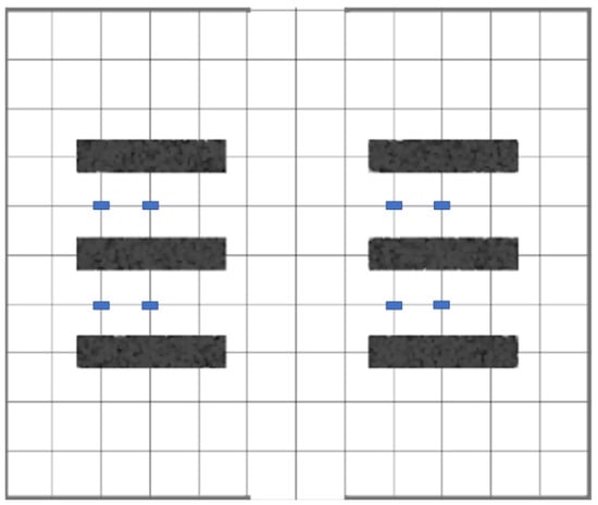
Figure 2.
Grid diagram of the working environment of AGVs.
2.2.2. Waypoint Fitting
Convolutional Neural Networks (CNN) possess a remarkable capability to capture both the global structure and detail features of an environment in heuristic learning, generating outputs with spatial structure. This trait aids in the smooth transition of heuristic values between adjacent configurations. Based on this, we apply convolutional neural networks to the heuristic function of the A* path planning algorithm, aiming to enhance the efficiency of path search for multi-AGV systems. As illustrated in Figure 3, this paper addresses the high time cost issue arising from collisions with obstacles requiring replanning during the cargo transportation process by AGVs in complex dynamic rail transport environments. It establishes a multi-AGV path planning task definition, taking into account the characteristics of the rail transport material handling environment. The grid information of the AGV environment and its starting position coordinates are input. Using the A* path algorithm as a baseline, by combining traditional path planning methods with deep learning approaches, it leverages automatically learned heuristic functions to minimize search costs in complex environments. It trains by minimizing the squared error between the predicted values of each waypoint on the path and the target cost values, eventually fitting an optimal path for each AGV with the minimum cumulative cost, achieving global path planning for AGVs. In this process, key waypoints on the path are defined as effective nodes, as shown in Figure 4. These nodes connect the start and end points, forming a set of nodes with the lowest cost, serving as the baseline heuristic true values during the training process.
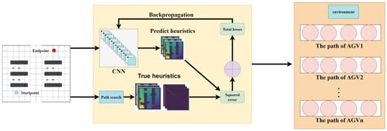
Figure 3.
Heuristic global programming algorithm based on waypoint fitting.
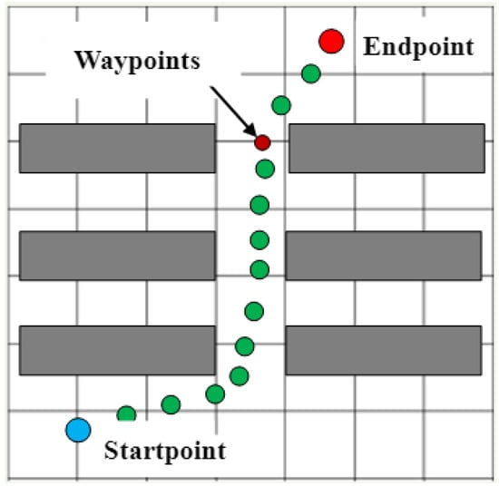
Figure 4.
Waypoints in the global path.
Define the search graph . In this graph, the function is used to expand the search edges, thereby accessing the successor edges and sub-vertices of vertex . Given that obstacles render some edges impassable, we validate the viability of each potential waypoint through the function ; this function returns true only if edge is not occupied by obstacles. Based on the environment , each candidate waypoint is evaluated using the search score function , and then they are added to the priority queue in order based on their scores. In each iteration, the waypoint with the highest score from queue is selected, the search scores of its sub-vertices are calculated, and they are added to the queue. This process continues until the target vertex is reached or the queue is empty. The path cost is calculated by accumulating the shortest path edge costs encountered during the search process. As defined by (7), the search heuristic function assigns an integrated score to each waypoint to balance efficiency and accuracy. This study, targeting environments containing obstacles, extracts feature maps and applies a Fully Convolutional Neural Network (FCNN) [25] to predict the heuristic value of each waypoint. Training is conducted by minimizing the squared error between the predicted value of each waypoint and its actual target cost value. The cost of a waypoint is defined as the cumulative cost from that point to the target point along the shortest path. Training is completed by minimizing the objective function defined in (8), with the goal of accurately predicting waypoint costs to optimize path planning. In the model, represents the target cost value, and acts as a mask function, assigning a value of 1 to each vertex on the path, to exclude invalid vertices, such as those occupied by obstacles or completely surrounded areas, when generating target values. To address the lack of supervisory signals for unvisited pixels, this study adopts a temporal difference method to compensate for the insufficient supervisory signals, as specifically defined in (9). Predicted values are iteratively updated through convolution with fixed kernels and biases, minimizing across the successor vertex axis, with the loss function defined in (10). Here, the value of is 1 when , otherwise, it is 0, and represents the weight coefficient for the temporal difference loss. This method refines the target cost estimation through multiple iterative updates. Training aims to plan the optimal global path for Automated Guided Vehicles (AGVs) by minimizing the squared error between the predicted values and the true target costs.
2.2.3. Conflict Resolution
In a multi-agent environment composed of Automated Guided Vehicles (AGVs), the starting position and the target position of each AGV are connected through a series of waypoints, defining the waypoint path set as . Here, represents the th waypoint on the path, where is the total number of waypoints, and respectively represent the two-dimensional position and direction of the AGV.
In the process of planning paths for each AGV individually, considering that all AGVs share the same graph , this study identifies and addresses two potential types of conflicts: vertex conflicts and edge conflicts. A vertex conflict occurs when two AGVs, and , occupy adjacent vertices at any time step , denoted as . Similarly, an edge conflict occurs between two consecutive time steps and if two AGVs come too close while traversing an edge, denoted as . Here, “too close” means the Euclidean distance between the two AGV centers is smaller than the sum of their speed-dependent safety radius, i.e., , where each radius combines the geometric footprint and a motion/uncertainty margin (see the subsection Collision model and choice of radius added after (12).
In a multi-AGV system, the function defines the two-dimensional coordinates of the waypoint for agent at time , where represents the specific position of the AGV in the environment and the subset of the environment it occupies. By checking the global path solutions in time order, we determine whether conflicts exist. Assuming a vertex conflict is detected, a method of constructing a binary constraint tree is adopted to generate two child nodes aimed at resolving the conflict. Specifically, in the first child node, a constraint is applied to to prevent it from being at position at time ; for the second child node, a corresponding constraint is applied to prevent it from being at position at time . A similar strategy is adopted to handle edge conflicts , and the search continues until a conflict-free solution is obtained.
2.2.4. Collision Model and Choice of Radius
We model each AGV at discrete step k as a disk centered at its geometric center with a speed-dependent safety radius:
where and are the length and width of AGV . The speed-dependent safety margin aggregates sensing–processing–actuation latency, braking capability, localization error, and an engineering clearance:
Here is the speed over the interval [k, k + 1]; is the measured end-to-end latency; is the guaranteed braking deceleration; is the 95th-percentile localization error; maps it to a conservative bound; and is a small engineering clearance (e.g., 0.05–0.10 m).
With these definitions, a vertex conflict at time k occurs if satisfies (16)
An edge conflict over [k, k + 1] occurs if the minimum distance between the two linear center trajectories on that interval violates the same bound as (17):
In implementation, we compute the exact segment–segment closest approach (checking endpoints and orthogonal projections), which is exact under linear interpolation.
Parameterization guideline
All terms are measurable on the platform:
: from (CAD/specs/measurements);
: from end-to-end timing tests;
: from controller/motor specs or braking tests;
: from calibration/alignment logs (95th percentile);
: per site policy/safety code (e.g., 0.05–0.10 m);
: 1–2 (e.g., 1.64 for a one-sided 95% bound).
If a speed limit is enforced, one may define a conservative constant radius for analysis:
Simulations and deployment use the speed-varying to reduce unnecessary conservatism.
Optional linear surrogate (for real-time checks):
To simplify runtime checks, we also use an upper-bounding linear surrogate on :
With chosen from , , , to ensure upper-bounds (15) over the operating speed range.
2.2.5. Reference Global Trajectory
For each AGV , the reference global trajectory is a kinematically feasible seed path computed before local optimization. It is built in three steps:
- 1. Graph search (rail-aware A)*
Build a yard graph G = (V, E) whose edges follow admissible rail/aisle centerlines. Assign edge costs
where penalizes sharp direction changes and κ(e) approximates curvature. Inflate static obstacles via a Minkowski sum by a conservative radius Rᵢᵗ to guarantee clearance as (21):
Run A* (admissible heuristic: geodesic/Euclidean) to obtain waypoints Wᵢ = { , …, }.
- 2. Curvature-constrained smoothing (geometric feasibility)
Fit a C2 spline sᵢ(ℓ) through Wᵢ subject to a turning-radius bound as (22)
producing a smooth centerline suitable for the platform’s minimum turning radius.
- 3. Time-parameterization (dynamic feasibility)
Compute speed v−ᵢ(t) along sᵢ(ℓ) with limits as (23):
Discretize with sampling period to obtain and .
- Safety Corridor used by the optimizer;
Given p−ᵢ(k), we define a tube (safety space) around the reference path as (24)
where Rᵢ(k) is the speed-dependent safety radius and ε > 0 is a small buffer. The optimizer constrains pᵢ(k) ∈ Cᵢ and uses the objective in Formula (26), whose two parts are
- (i).
- Smoothness: a penalty on input increments
- (ii).
- Tracking: a penalty on deviations from the reference (e.g., position and speed).
2.2.6. Trajectory Optimization
In this section, we optimized the obtained discrete paths, converting them into smooth trajectories. Specifically, a time stamp is assigned to each waypoint in the global path for each Automated Guided Vehicle (AGV). Thus, the global path is transformed into a reference trajectory , where each segment on the original global path is evenly divided into parts. At the same time, the kinematic model for each AGV is defined as (25)
In this framework, the state of an AGV is defined as its two-dimensional position and orientation , . Here, and respectively represent the AGV’s linear and angular velocities. The optimal smooth trajectory is defined as the set , and the corresponding nonlinear optimization problem can be formalized as (25)
where and . Here, and are two positive definite weight matrices, respectively. Formula (8) must satisfy conditions such as (27)–(31)
In this framework, represents the safety space considered when extending the global path. According to Formula (14), the objective function contains two main parts. The first part promotes the smoothness of the trajectory by imposing a penalty on the differences between consecutive control inputs. The second part considers that the reference global trajectory of each Automated Guided Vehicle (AGV) already represents a feasible solution. To maintain feasibility, we penalize deviations from a precomputed reference global trajectory , which we construct by: (i) running a rail-aware A* search on the yard graph to obtain a waypoint sequence that avoids inflated static obstacles, (ii) smoothing it into a curvature-constrained spline, and (iii) time-parameterizing it under the platform’s speed/acceleration limits; see the subsection “Reference global trajectory” for details.
At each time step , the state transition is given by , where the nonlinear model is its discrete-time version. The position of each waypoint on the trajectory is constrained by the safety space which is settled by constraint condition . In the control input for each AGV, is limited by the range of its physical capabilities. Additionally, the requirement to maintain a safe distance between each pair of AGVs is represented by .
Trajectory optimization primarily focuses on the constraints between AGVs (constraint 8f). Since the optimal trajectory approaches the reference trajectory according to the cost function (8a), the constraints between AGVs can be analyzed based on the reference global trajectory . At each time step , a search for constraint satisfaction is conducted by analyzing the combination of three AGVs with the aim of satisfying (32).
In this section, we introduce a threshold to judge the proximity of three AGVs to each other within a specific time step, where each triplet represents the closeness situation of three AGVs at that time step. In the discrete path planning stage, we can only confirm that four AGVs simultaneously satisfy the condition of (20) when the four AGVs are located at the four vertices of the same grid cell.
When AGVs in a triplet are assigned different priorities, the AGV with higher priority will plan its trajectory first. Subsequently, these trajectories will act as hard constraints for the optimization problem of AGVs with lower priority. In this case, the original problem may no longer have a feasible solution. Therefore, it is suggested to consider the AGVs within a triplet as a whole and assign them the same priority. A list is defined to represent all triplets that satisfy the condition of (20).
If the number of AGVs in the workspace is large, will contain a large number of elements, making the same AGV appear in multiple triplets. In such cases, it is not straightforward to group AGVs. Each triplet represents a scenario where three AGVs are close to each other, and if the same triplet appears multiple times in , it indicates that the trajectories of these three AGVs are highly coupled. Based on this, we propose an algorithm to assign priorities based on the frequency of triplets’ occurrences.
Initially, the element with the highest frequency of appearance in is designated as the first priority group. Since the AGVs in this new group may appear in other triplets in , all these AGVs will be removed from , generating a new list . Consequently, the elements in may contain three, two, or just one AGV. Next, the element with the highest frequency of appearance in the new list is chosen as the second priority group, and this process is repeated until the list is empty. If an AGV does not have significant coupling with other AGVs, it will not appear in the original list , and such AGV is considered as a separate AGV group, assigned the lowest priority.
We adopt a priority-based, group-wise optimization. Let the 8 AGVs be partitioned into four priority groups , , , in descending order of priority, e.g., . At iteration , we optimize trajectories for all AGVs simultaneously, while keeping the already-optimized higher-priority trajectories fixed and treating them as moving obstacles. The current group must satisfy (i) its own dynamic and smoothness constraints, (ii) intra-group collision avoidance, and (iii) inter-group collision avoidance with all higher-priority AGVs:
Figure 5a–d illustrate one complete priority-based optimization process from the highest- to lowest-priority AGV groups. Gray squares represent static obstacles, arrows denote motion directions, and numeric labels mark AGV IDs. At each iteration, the colored curves are the trajectories currently optimized, while black curves show higher-priority trajectories that have already been fixed. The optimization enforces feasibility through distance constraints with respect to both static obstacles and previously fixed agents.
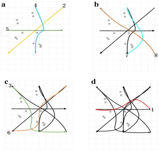
Figure 5.
Example of priority-based track optimization. (a) First iteration: {2,4,5} optimized against static obstacles only. (b) Second iteration: {7,8} optimized while avoiding fixed {2,4,5}. (c) Third iteration: {3,6} optimized while avoiding {2,4,5} and {7,8}. (d) Final iteration: AGV 1 optimized while avoiding all prior groups.
To operationalize the priority-based smoothing in Section 2.2.5, we first fix global reference paths and define the safety set . AGVs are partitioned into priority groups using the triplet-frequency rule derived from the proximity test in (33). We then iterate from high to low priority: trajectories of already-solved (higher-priority) groups are frozen as hard constraints, and the current group solves the smoothing program in (27) over horizon under the dynamics (Equation (26)), boundary and input/state bounds ((28)–(31)), and both static-obstacle clearance and cross-group separation (32). If infeasible, we apply standard soft-constraint slack and re-solve. This yields a set of smoothed, feasible, and collision-free trajectories that remain close to while enforcing inter-AGV safety. Algorithm 1 lists inputs/outputs and symbols; Algorithm 2 gives the stepwise pseudo-code aligned with ((26)–(31)); Figure 5 illustrates the grouping and iterative solution process.
| Algorithm 1 Multi-AGV Smooth Trajectory Optimization |
| Require: Global reference paths , initial states ν, horizon length H |
| Ensure: Smoothed and collision-free trajectories {, } |
| 1: Initialize trajectories {} for all AGVs i |
| 2: repeat |
| 3: for each AGV i = 1,..., n do |
| 4: Set initial state , terminal state |
| 5: for each step j = 1,..., H do |
| 6: Update dynamics: |
| 7: Enforce safety set constraint: |
| 8: Bound control inputs: |
| 9: end for |
| 10: Check inter-AGV separation: |
| 11: end for |
| 12: Compute cost function: |
| 13: Update trajectories { , } based on optimization results |
| 14: until convergence or max iterations |
| 15: Return optimized trajectories { , } |
| Algorithm 2 Priority-based Multi-AGV Trajectory Smoothing |
| Require: Global reference paths , safety set S, priority groups {,…, }, horizon length H |
| Ensure: Smoothed and collision-free trajectories } |
| 1: Initialize fixed-trajectory set H ← ∅ |
| 2: for each priority group k = 1,…,m (high → low) do |
| 3: Add trajectories of higher-priority groups to hard set: |
| H ← |
| 4: for each AGV i ∈ do |
| 5: Time-parametrize reference path : H using uniform subdivision |
| 6: Formulate optimization objective: |
| 7: Apply constraints: |
| (a) Dynamics: |
| (b) Input/state bounds: |
| (c) Static-obstacle clearance: |
| (d) Cross-group separation: |
| 8: Solve optimization problem using SQP/interior-point: |
| ) ← argmin objective under constraints |
| 9: end for |
| 10: If infeasible: |
| introduce slack ξ to soften non-critical constraints with penalty, |
| re-solve; if still infeasible, apply trajectory shifts/reduced horizon |
| 11: Add optimized group trajectories { } to H |
| 12: end for |
| 13: Return all optimized trajectories } |
2.2.7. Experimental Results and Analysis
- 1. Multi-AGV global path planning results
Figure 6a,b depicts a back-of-house material-transportation system in a subway environment: autonomous carts move spare parts, consumables, and tools between storage rooms, platform-side service bays, and equipment rooms via service aisles that run alongside but never on the rail tracks. In the map, rail tracks are non-traversable regions and are rendered as regularly spaced rows of gray dots indicating track centerlines; they serve as anatomical references of the station layout and as prohibited areas for AGVs. Static obstacles comprise platform edges, load-bearing columns, equipment cabinets/racks, walls, stairway footprints, and other permanent fixtures; these are shown as scattered gray dot clusters surrounding the tracks. For collision checking during planning, all static obstacles are inflated by a conservative clearance (Minkowski sum) consistent with the speed-dependent safety radius defined earlier.
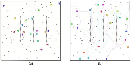
Figure 6.
Global path planning trajectory diagram for multiple AGVs. (a) Initial state. (b) Planning Results. Colored rectangles represent the AGVs, with bold solid lines of the same color indicating their trajectories, and same-colored squares at the endpoints denoting the targets. Gray dots/point clusters represent rail tracks and static obstacles, respectively.
Each AGV is modeled as a rectangle (length Li, width Wi) with nonholonomic (differential-drive or skid-steer) kinematics subject to platform limits (maximum speed/acceleration and lateral acceleration). Collision avoidance uses the speed-dependent safety radius introduced in an earlier section; two agents are considered safely separated when . Start poses are sampled around the tracks and in remote service areas to create heterogeneous traffic conditions. Each AGV is assigned a unique docking goal (a storage bay or platform-side service point) so that all routes are distinct and potential conflicts are meaningful.
In Figure 6, each AGV’s footprint is shown as a colored rectangle; its planned carrying trajectory is the thick polyline in the same color with arrowheads indicating motion direction. The colored square at the end of each polyline marks the final docking pose. To ensure legibility on print and screen, we render trajectories with a line width of at least 2.5 pt, use a high-contrast color palette, add arrowheads approximately every 15–20 m, and apply slight transparency where paths overlap; for the densest areas, we provide zoomed insets (not shown to scale) so that minimum-distance separations and obstacle clearances are visually verifiable. Under this setup, the figure demonstrates how each AGV leaves its start, navigates around static obstacles while respecting track prohibition, and reaches its randomly assigned target without collision.
- 2. Conflict resolution
Further, Figure 7 reveals the dynamic process of conflict resolution in a multi-AGV system. By marking the AGVs around the imminent conflict point with red and black circles, respectively, we observed that at t = 3 s, two AGVs approached the conflict point. As time progressed, the purple AGV detected a potential conflict at t = 4 s and chose to temporarily wait, allowing the orange AGV to pass first at t = 5 s. Once t = 6 s passed and the orange AGV safely went through, the purple AGV continued its path, successfully avoiding the conflict. Another scenario occurred at t = 8 s, where the orange AGV and the pink AGV, marked with a blue circle, were about to conflict. The pink AGV avoided the conflict with the orange AGV by executing a quick retreat at t = 10 s.
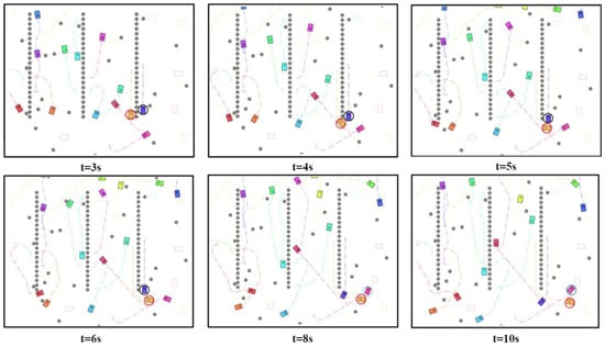
Figure 7.
Multi-AGV path conflict resolution diagram.
- 3. Trajectory optimization results
Moreover, Figure 8a showcases the results of trajectory optimization based on modeling the AGV working environment. By smoothing the trajectories of discrete paths, we positioned some AGVs around the tracks as starting points, while others are placed outside the tracks, acting as temporary standby AGVs. Ultimately, Figure 8b presents a three-dimensional visualization of the optimized trajectories, intuitively demonstrating how AGVs efficiently navigate around obstacles in a complex environment to reach their predetermined targets.
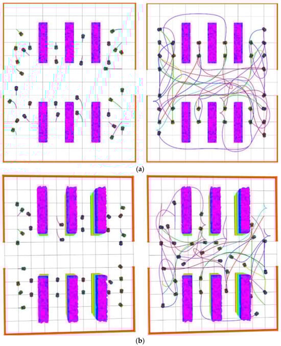
Figure 8.
Optimization effect of multi-AGV global path planning. (a) Two-dimensional effect; (b) Three-dimensional effect.
2.3. Research on Environmental Perception Algorithm Based on Multi-Sensor Feature Fusion
In the orbital transportation environment, Automated Guided Vehicles (AGVs) are responsible for tasks such as cargo handling. Given the limited dwell time of trains at each station, AGVs need to complete tasks quickly and be capable of real-time obstacle avoidance. To enhance transportation efficiency, AGVs must possess autonomous path planning capabilities. This study utilizes the built-in sensor equipment of AGVs to perceive the surrounding environment and their own state, assisting AGVs in making intelligent decisions to cope with the complexity and variability of the environment. This enables AGVs to plan an optimal path from the starting point to the destination in a complex environment filled with dynamic obstacles.
2.3.1. Visual Feature Processing Based on Dual Modules
In modern automated logistics systems, traditional Automated Guided Vehicles (AGVs) rely on predetermined paths or are guided by ground wires to perform handling tasks [26]. However, this reliance on highly maintained path planning not only increases significant maintenance costs but also leads to queue congestion among AGVs during task execution, resulting in reduced efficiency. To address these issues, this study developed a comprehensive environmental perception model that integrates point cloud data generated by LiDAR, the status information of AGVs, and visual images captured by front-mounted cameras. The model uses deep reinforcement learning techniques to provide extensive perception capabilities for the path planning of multiple AGVs.
Figure 9 presents the proposed multi-sensor data fusion-based environmental perception framework of this study, aimed at enhancing the accuracy and response speed of AGVs’ perception of the surrounding environment. As shown in Figure 9a, the simulated AGV equipped with cameras for real-time obstacle avoidance is demonstrated. For this purpose, it is necessary to train the AGV so that it can accurately perform scene classification based on the visual information captured by the camera, identifying other AGVs, static obstacles, and target points. The goal is to ensure that the AGV can reach the specified destination smoothly without collisions. The image resolution captured by the AGV’s front-mounted camera is 768 × 1024 × 3. To improve the efficiency of path planning in obstacle avoidance training while retaining image content, the original images are processed into grayscale images of 80 × 80 × 3 before entering the shared convolutional layers.
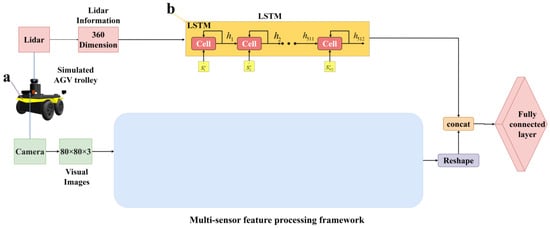
Figure 9.
An environment-aware framework based on multi-sensor feature fusion: (a) Simulated AGV trolley; (b) LSTM module.
We designed and implemented a multi-sensor data processing framework that adopts a dual-branch structure, sharing input data and several convolutional layers. As shown in Figure 10, we utilized a Siamese Deep Convolutional Neural Network (DCNN) architecture, which processes inputs from both the AGV environmental information perception module and the scene classification module simultaneously through shared convolutional layers, further extracting image information captured by the AGV camera. This approach enables us to distinguish between different types of obstacles and targets, and integrates LiDAR and camera features with the AGV’s own information to form a comprehensive environmental perception model. As shown in Figure 10a, the shared convolutional layers, consisting of multiple convolutional and max pooling layers, aim to extract key features from the input images, serving as input for the AGV’s environmental perception and scene classification modules. The purpose of this design is to enhance the model’s processing efficiency and achieve efficient memory usage and reduced inference time, without compromising the prediction accuracy of the two branches. By integrating the AGV’s environmental information and scene semantic segmentation, the framework achieves precise localization of the AGV and effective classification of the visual information obtained through the front-mounted camera. The architecture of the AGV environmental information perception module, as shown in Figure 10b, includes three convolutional layers, two max pooling layers, two global average pooling layers, and one fully connected layer. This module aims to precisely locate the AGV within the captured scene, especially determining the AGV’s orientation angle and position relative to the current waypoint, as illustrated in Figure 10d. Through the environmental information perception module, the AGV’s current self-information (, ) can be obtained, where represents the distance between the AGV and the nearest waypoint on the global path, and indicates the orientation angle of the AGV relative to that waypoint. As demonstrated in Figure 10c, Atrous Spatial Pyramid Pooling (ASPP) technology is employed. This technique captures object and image context information at multiple scales using dilated convolutional layers with different sampling rates. This method allows the model to integrate multi-scale features into its effective receptive field, thereby reconstructing dense features from the sparse outputs generated by the network. As shown in Figure 10e, this module aims to achieve pixel-wise segmentation of the incoming scene, subsequently classifying the scene content by labels: dynamic carts, static obstacles, and target points. Specifically, dynamic obstacles are marked in red, static obstacles in blue, and target points in green for visual distinction.
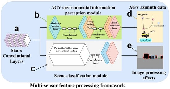
Figure 10.
Multi-sensor feature processing framework: (a) Shared convolutional layers; (b) AGV environmental information perception module; (c) Scene classification module; (d) AGV azimuth data; (e) Image processing effects.
2.3.2. LiDAR Information Processing
In this study, the simulated Automated Guided Vehicle (AGV) is equipped with LiDAR and generates point cloud data. Due to the long sequence characteristic of point cloud data over time steps, Long Short-Term Memory (LSTM) networks are used for processing, thus extracting distance and angle information about target points and obstacles, as shown in Figure 10b. The LSTM network starts from an initial empty state, receiving the observation state at the first time step to generate the hidden state vector . Thereafter, the network generates a new hidden state based on and , repeating this process until the AGV reaches its destination. In this study, the LSTM network’s cell units are set to 512 to handle the 360-degree point cloud information output by the LiDAR, with an update frequency set at 50 Hz and a detection range of [−90°, 90°]. Considering that the AGV’s own information (such as linear velocity and angular velocity is also based on time steps, this study also employs LSTM networks to process both the LiDAR point cloud information and the AGV’s linear and angular velocities and , to achieve more accurate environmental perception and motion control. As the AGV moves from its starting position to its destination, the environmental perception module can obtain and process the state information of the surrounding environment in real-time, providing a real-time perception field of view for the AGV. Figure 11 shows an example of the real-time perception field of view captured by the AGV through the environmental perception module, demonstrating how the AGV can effectively identify and respond to environmental changes along its path.
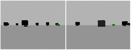
Figure 11.
Real-time capture of environment awareness.
We fuse LiDAR and camera cues in a probabilistic occupancy grid defined on the ground plane. Let ccc index a grid cell and denote its log-odds occupancy at time . The fusion update is:
where are modality weights, mitigates stale evidence, and clip(·) bounds log-odds to avoid numerical saturation.
LiDAR inverse model, for each ray, all cells before the first return are treated as free and the impact cell as occupied:
With , . We down-weight low-quality returns using range- and incidence-dependent confidence.
Camera inverse model: The image is semantically segmented to produce per-pixel class posteriors. Using the calibrated homography from image to ground plane, obstacle probabilities are projected to grid cells. For cell c, the camera contribution is:
where is an automatically estimated quality factor that down-weights unreliable image evidence (e.g., motion blur, low light, glare, heavy occlusion), computed from softmax entropy, optical-flow residuals, and exposure statistics.
Decision rule and persistence:
Occupancy probability with the logistic function. We use hysteresis thresholds (e.g., , ):
- If for consecutive frames mark occupied.
- If for consecutive frames, mark free.
- Otherwise mark unknown and treat as a soft cost in planning.
Contradictory observations:
LiDAR says occupied, camera says free. We rely on LiDAR unless LiDAR confidence is low (e.g., grazing incidence, max range) and the camera reports high-confidence free for frames. This implements a conservative bias that prevents spurious clearing.
Camera says obstacle, LiDAR sees through (free). This is common under visual occlusion (e.g., posters, reflections). We require temporal persistence of the camera’s obstacle class and geometric consistency after ground projection; if LiDAR repeatedly clears rays along rays and the camera’s confidence is unstable, we keep the cell unknown (soft cost) rather than hard-occupied.
Static vs. dynamic classification: Cells that remain occupied for frames with near-zero optical-flow parallax are tagged static and inflated (Minkowski sum) by the safety radius; otherwise, they are treated as dynamic and enter the planner’s dynamic cost layer.
Gating, synchronization, and outlier rejection: All measurements are time-synchronized to the AGV clock; extrinsics between LiDAR, camera, and base are calibrated once and refined online. We reject visual outliers via class-wise morphological filtering and entropy gating; LiDAR outliers are filtered by statistical outlier removal and range-dependent intensity checks. Raycasting enforces free-space carving before hits to prevent false positives behind confirmed frees.
Planner interface: The fused map exposes a hard occupancy layer (binary) and soft cost layers (unknown/dynamic). The global planner forbids hard cells; the local/trajectory optimizer penalizes traversal of soft cells but will reroute if necessary. This separation ensures safety under disagreement while avoiding over-conservatism.
Typical parameters (unless otherwise specified): , , , , , , , , .
2.4. Research on Dynamic Path Planning of Multi-AGV Based on Deep Reinforcement Learning Under Global Guidance
Traditional multi-agent planning algorithms typically represent agents with simple shapes, such as rectangular boxes, and most of these algorithms are only applicable to static and fully known planning scenarios. However, this study focuses on the operational environment of AGVs (Automated Guided Vehicles) in the rail transit domain, where not only static obstacles need to be considered but also dynamic obstacles, such as other AGVs. Moreover, existing AGV path planning algorithms in domains like warehouse logistics are not suitable for the rail transit environment, demonstrating their limitations.
This study proposes an innovative AGV path planning method for rail transit applications. By designing novel reward functions and incorporating deep reinforcement learning, we allow AGVs to learn through interaction with the environment without relying on predefined training sets. Although this process may face challenges such as delays and noise, it still offers significant advantages over traditional multi-agent planning algorithms. This paper particularly emphasizes the integration of global guidance and multi-sensor feature fusion techniques within the deep reinforcement learning framework, to accelerate the model’s convergence rate and effectively achieve dynamic obstacle avoidance among multiple AGVs, optimizing path planning.
For static obstacle detection, this study adopts a one-time global planning strategy, ensuring that AGVs can reach their target locations via an obstacle-free path. In contrast, when facing dynamic obstacles such as other AGVs, this method predicts their motion trajectories to assess collision risks. While the artificial potential field method [27], the extended Rapidly exploring Random Trees (RRT*) [28], and the dynamic D* algorithm [29] are typical methods for solving planning problems in dynamic environments, each has its limitations. For example, the artificial potential field method is prone to becoming stuck in local minima, and the D* algorithm is inefficient when dealing with changes in nodes far from the AGV.
2.4.1. Multi-AGV Dynamic Path Planning and Design
In the rail transit material handling environment, multiple AGVs work in parallel, transporting goods and serving as dynamic obstacles to each other. In environments where a large number of AGVs operate simultaneously, it is crucial to achieve collision-free delivery to the target points. Addressing the avoidance of dynamic obstacles (such as other AGVs) in a multi-AGV operational environment, as illustrated in Figure 12, this paper presents a study on multi-AGV dynamic path planning under global guidance based on deep reinforcement learning. Integrating a deep reinforcement learning model with global guidance, a differentiated reward and punishment method for multi-AGV dynamic planning is trained: the multi-AGV paths output by the deep convolutional model from the first part of the study serve as global guidance. Through the environmental perception model detailed in the second part of the study, real-time motion and environmental information fed back by AGVs are obtained to determine the relative positions of waypoints and set short-term goals. Combined with decision-making by the deep reinforcement learning model, corresponding rewards or punishments are applied to AGVs’ movements, and the state after each decision is stored in the experience replay pool as a training sample for future use. Different rewards or punishments are given to AGVs based on the outcomes of each navigation attempt. Using initial paths obtained by traditional algorithms as a baseline to comprehensively guide the AGVs’ deep reinforcement learning accelerates the convergence speed of the deep learning model. Through a custom-designed reward function, autonomous vehicles can approximately follow the initial paths to quickly reach their targets, achieving relatively smooth trajectories and high navigation efficiency.
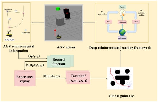
Figure 12.
A multi-AGV path planning framework based on deep reinforcement learning under global guidance.
In considering the path planning for Automated Guided Vehicles (AGVs), this study treats other AGVs as dynamic obstacles and employs the Deep Q-Network (DQN) [30] as the framework for reinforcement learning (RL). This paper has developed a multi-AGV path planning framework based on deep reinforcement learning, which operates under the guidance of a global planner to optimize AGVs’ dynamic obstacle avoidance strategies. As illustrated in Figure 12, the framework perceives environmental states through deep learning (DL) techniques and decides the AGV’s action strategy based on this. Whenever an AGV executes an action, it enters a new state , and receives a reward or punishment according to a specific reward function , thereby generating a new sample . These samples are collected into an experience pool, providing historical data support for subsequent training. Through this method, this study aims to achieve efficient path planning and obstacle avoidance for AGVs in complex dynamic environments, reinforcing their autonomous navigation capabilities. The utilization of the experience pool ensures that the model can learn from past interactions and accelerate the learning process and improve decision quality through iterative improvements.
2.4.2. Reward Function Design
Based on the AGV’s own environmental information parameters obtained by the AGV environmental information perception module, and after the introduction of global guidance, the target point in the reward function is set as the nearest waypoint. As shown in Figure 13, this study defines the relative distance and heading deviation angle between the Automated Guided Vehicle (AGV) and the target waypoint at continuous time steps and as , and , , respectively. Meanwhile, the relative distance and heading deviation angle between the AGV and obstacles at corresponding time steps are defined as , and , .
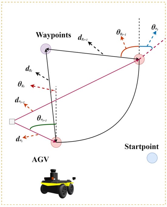
Figure 13.
AGV environment information.
The design of the reward function in this study is based on the criteria of (37). When an AGV collides with an obstacle, the reward function = ; when the AGV reaches within 0.5 range of the target point, = ; under other conditions, the reward function = , which is determined by the relative distance between the AGV and the target, the change in heading deviation, as well as the distance between the AGV and obstacles, and the change in heading deviation.
The reward function has been carefully designed to guide Automated Guided Vehicles (AGV) to efficiently plan paths and avoid obstacles. The reward factor includes several parts, as follows: represents the reward induced by changes in the distance between the AGV and the target. When the distance to the target decreases, provides a positive reward, motivating the AGV to move closer to the target. is based on changes in the heading deviation angle between the AGV and the target. A decrease in the heading deviation angle means that the AGV is moving in the correct direction, and therefore, rewards this positive change. and reflect the rewards associated with changes in the relative distance and course angle to obstacles, respectively. Specifically, is a negative value, designed to increase the penalty when the AGV is too close to an obstacle, thereby encouraging the AGV to maintain a safe distance. , on the other hand, rewards the AGV for making course adjustments to avoid obstacles. Significant penalties and large rewards are, respectively, applied when the AGV collides with an obstacle or successfully reaches the target, marking the end of the current Episode and initiating a new learning process. Through this reward mechanism, this study aims to optimize the AGV’s path planning strategy, achieving effective obstacle avoidance and target navigation in complex environments.
3. Experimental Results and Analysis
To intuitively and objectively evaluate the proposed method’s effectiveness and advantages in dynamic multi-AGV path planning and obstacle avoidance, we constructed five canonical benchmark environments, each measuring 30 m × 30 m (Figure 14). In every environment, ten start–goal pairs were randomly sampled; the specific start and goal coordinates for the focal AGV are reported in Table 1, thereby ensuring diverse and representative test conditions.
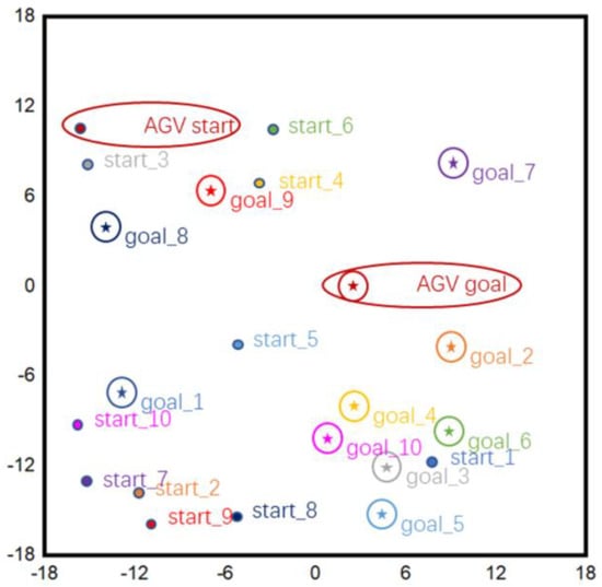
Figure 14.
Schematic diagram of any starting point and target point.

Table 1.
Starting Point Coordinates of the Main AGV.
By contrasting the trajectories produced by the proposed method (Figure 15a) with those generated by the conventional Artificial Potential Field (APF) approach (Figure 15b), distinct differences in performance become evident. In Figure 15a, the trajectory generated by our algorithm is shown, with the primary AGV’s path highlighted in red. The results indicate that the proposed approach can effectively anticipate the motion of dynamic obstacles and proactively adjust its route, yielding shorter and smoother paths. Conversely, as seen in Figure 15b, the APF method lacks predictive awareness of obstacle dynamics, leading to frequent detours and large fluctuations in the trajectory. This significantly increases path length and reduces smoothness. The underlying reason is that APF relies solely on real-time calculations of attractive and repulsive forces, making it prone to local minima and unstable paths, especially in environments with dense dynamic obstacles.
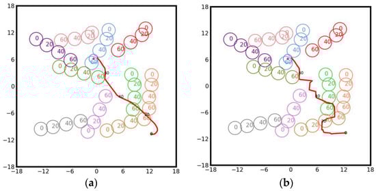
Figure 15.
Contrasting AGV trajectories under the proposed framework and the conventional APF method: (a) Our algorithm; (b) Artificial potential field algorithm.
To quantitatively assess and contrast the path planning capabilities of the two methods, Figure 16 presents a detailed comparison across four key metrics: obstacle avoidance, computation time, path length, and trajectory smoothness. As shown in Figure 16a–d, we conduct a systematic comparison between the proposed method and the Artificial Potential Field (APF) baseline across five benchmark maps (Map 1–Map 5). First, in obstacle-avoidance capability (Figure 16a), measured by collision count, the proposed method yields markedly fewer collisions on every map, with an average reduction of about 70%, indicating stronger handling of dynamic obstacles and higher system safety. Second, in computational efficiency (Figure 16b), the average planning time of the proposed method is approximately 130–150 ms, whereas APF requires about 205–230 ms, a reduction of roughly 25–30%, satisfying real-time planning requirements in dynamic environments. Third, in path quality (Figure 16c), the shortest path length produced by the proposed method is about 28–30 m, compared with 32–35 m for APF, a mean shortening of about 10–15%; this effectively suppresses the oscillations typical of APF and reduces AGV energy consumption. Finally, for trajectory smoothness (Figure 16d), quantified by the root-mean-square (RMS) curvature, the proposed method achieves about 0.23–0.25 versus 0.34–0.37 for APF, an average decrease of 20–25%, yielding smoother motion, fewer abrupt turns, and improved control stability. Taken together, the integration of deep reinforcement learning with multi-sensor fusion confers clear advantages over APF in safety, real-time performance, path optimization, and trajectory smoothness, demonstrating strong potential for deployment in complex, highly dynamic environments.
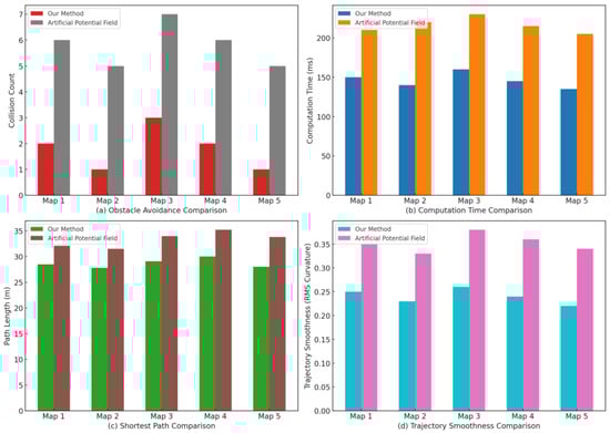
Figure 16.
Performance comparison in obstacle avoidance, efficiency, path length, and smoothness.
3.1. Static Evaluation on the Maze Benchmark Map
To further demonstrate the generalization ability and robustness of the proposed dynamic path planning approach under standardized testing conditions, this study adopts the publicly available Maze Benchmark Map for comparative experiments. Owing to its intricate layout and dense obstacle distribution, this benchmark is widely recognized for assessing the optimality and convergence properties of path planning algorithms in static environments and is considered highly representative.
As shown in Figure 17, on the standard 50 × 50 maze grid (gray cells: static obstacles; blank cells: traversable space), the start S is placed at the upper-left corner and the goal G at the lower-right. The three planning results indicate that GG-DRL (red solid line) follows the diagonal corridor with a shorter and smoother feasible path, reliably avoiding dead ends and bottlenecks with fewer turns and minimal detours; DDPG (black dashed line) reaches the goal but exhibits local back-and-forth motion and redundant detours in complex regions, yielding a longer and less smooth trajectory; RRT (blue dash-dot line), due to its randomized sampling, produces a path with zig-zag segments and large detours, often backtracking after exploring multiple branches. Overall, GG-DRL demonstrates superior reachability, path optimality, and trajectory smoothness, whereas DDPG and RRT, although feasible, are limited by local oscillations and random wandering, with lower stability and consistency.
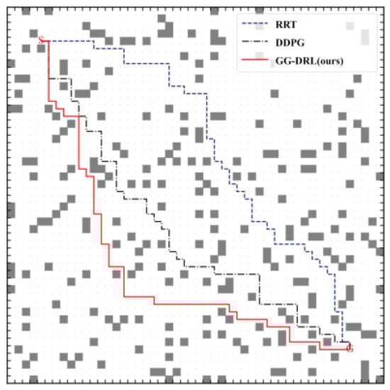
Figure 17.
Path Comparison of Planning Algorithms on the Standard Maze Map.
The experiments were carried out on the standard Maze Benchmark Map. For each algorithm, 30 independent training runs were executed, with 1000 iterations per run. To provide a comprehensive evaluation, four performance indicators were measured: path length, computation time, obstacle avoidance frequency, and trajectory smoothness.
As shown in Table 2, we evaluated three algorithms on the standard maze benchmark over 30 independent trials, using four metrics: path length, computation time, obstacle-avoidance frequency, and trajectory smoothness. All methods achieved the shortest attainable path of 80 units, indicating convergence to the global optimum in a static environment. However, in terms of statistics, our GG-DRL achieved the best mean path length (80.12 units), outperforming DDPG (80.37 units) and RRT (84.00 units); its maximum path length was only 85 units (versus 86 for DDPG and 87 for RRT), yielding a narrower spread and thus better optimization stability and consistency.
Table 2.
Comparison of Path Planning Algorithms on the Standard Maze Map (30 Trials).
Regarding computational efficiency, GG-DRL attained a mean planning time of 10.94 s, markedly lower than DDPG (62.38 s) and RRT (296.08 s), and exhibited the tightest time range (10.1–11.8 s), reflecting fast and stable convergence suitable for real-time planning. Measured by contact/collision counts, the obstacle-avoidance performance of GG-DRL averaged 5.2, lower than DDPG (9.8) and RRT (24.3), indicating a larger safety margin and stronger adaptability to complex corridors. For trajectory quality, GG-DRL achieved a mean smoothness (0–1 normalized) of 0.85, exceeding DDPG (0.81) and RRT (0.78), with a min–max range of 0.77–0.90, demonstrating higher controllability and execution smoothness. Overall, GG-DRL surpasses the baselines across all four indicators—path optimality, real-time performance, obstacle-avoidance safety, and trajectory smoothness—while also exhibiting smaller statistical variation and stronger robustness.
3.2. Dynamic Environment Under 10, 20, and 30 Obstacles
In this study, three dynamic test scenarios of different complexity levels were designed to evaluate the adaptability and robustness of path planning algorithms. Specifically, 10, 20, and 30 moving obstacles were randomly placed on static obstacle maps, thereby constructing dynamic environments as illustrated in Figure 18. Each dynamic obstacle followed the shortest route between a predefined start and goal—calculated using the A* algorithm—moving back and forth along this path to emulate continuously changing interference sources similar to those encountered in real-world operations.
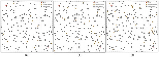
Figure 18.
Test Environments with Varying Dynamic Obstacle Densities: (a) Low-Complexity Test Scenario with 10 Dynamic Obstacles; (b) Medium-Complexity Test Scenario with 20 Dynamic Obstacles’ (c) High-Complexity Test Scenario with 30 Dynamic Obstacles.
Figure 18 depicts three dynamic environments with increasing difficulty. In panel (a), only 10 moving obstacles are present, producing a relatively open scene in which interference to planning is mild and the AGV can execute ample detours and simple avoidance maneuvers. Panel (b) elevates the density to 20 moving obstacles, markedly complicating the scene and forcing more frequent evasive actions and online re-planning, thereby probing each method’s adaptability and responsiveness. Panel (c) further intensifies the setting to 30 moving obstacles; the resulting high-dynamics, high-uncertainty conditions leave narrow safety margins and make collision avoidance considerably harder, placing stricter demands on perception, decision-making, and trajectory robustness. By scaling the number of movers from 10 to 30 across these scenarios, we can systematically assess algorithmic performance and stability under progressively more challenging dynamic environments.
In the test scenario with 10 dynamic obstacles, the performances of RRT, DDPG, and the proposed GG-DRL algorithm were compared across four evaluation metrics: path length, computation time, obstacle avoidance frequency, and trajectory smoothness. The detailed results are provided in Table 3.
Table 3.
Statistical Performance Metrics in a 10 Dynamic Obstacles Scenario.
As shown in Table 3, we compare RRT, DDPG, and GG-DRL (ours) over 30 runs using four indicators: path length, computational time, obstacle-avoidance frequency, and trajectory smoothness. All three methods approach the shortest attainable path under this low-dynamics setting—the minimum path length lies in the 80–81-unit range (RRT: 81; DDPG/GG-DRL: 80)—indicating that each can approximate the global optimum in static portions of the map. In terms of averages, RRT and GG-DRL report 81.7 and 81.9 units, respectively, both clearly below DDPG’s 82.1 units. The variation bands are also tight (GG-DRL: 80–84; DDPG: 80–84; RRT: 81–83), suggesting broadly comparable path optimality at this difficulty level, while GG-DRL gains more on efficiency and safety.
For computational efficiency, GG-DRL achieves a mean planning time of 12.08 s (min/max 11.29–12.64 s), substantially faster than DDPG’s 66.19 s (63.54–70.78 s) and RRT’s 307.21 s (300.08–323.78 s). On average, this corresponds to ~81.75% and ~96.07% reductions versus DDPG and RRT, respectively, with the narrowest spread among the three—evidence of faster, more stable convergence and stronger real-time suitability in this dynamic scene.
Measured by contact/collision counts, obstacle avoidance likewise favors GG-DRL: a mean of 4.0 events versus 4.8 (DDPG) and 5.1 (RRT), with a tighter min–max band (2–5 for GG-DRL; 3–6 for DDPG; 3–7 for RRT). This indicates a steadier, less intervention-heavy avoidance strategy that effectively reduces potential conflicts under sparse dynamic interference. Regarding trajectory smoothness (normalized 0–1), GG-DRL attains the best average (0.87, range 0.77–0.92), surpassing DDPG (0.85, 0.75–0.92) and RRT (0.84, 0.74–0.90). The resulting paths are more continuous with fewer abrupt turns, which benefits control stability, energy use, and mechanical wear.
Overall, in the “10 dynamic obstacles” scenario (low–moderate dynamic complexity), path optimality is broadly comparable across methods, but GG-DRL consistently leads in computational efficiency, avoidance reliability, and trajectory smoothness, while exhibiting smaller statistical variance and stronger robustness.
In the 20-obstacle dynamic environment, the study further compared the performance of RRT, DDPG, and the proposed GG-DRL algorithm across four metrics: path length, computation time, obstacle avoidance frequency, and trajectory smoothness. The results are summarized in Table 4.
Table 4.
Statistical Performance Metrics in a 20 Dynamic Obstacles Scenario.
As shown in Table 4, under a medium-complexity setting with 20 moving obstacles, we evaluated RRT, DDPG, and GG-DRL (ours). For path length, all three methods approach the global optimum at the minimum (RRT/DDPG/GG-DRL = 81/80/80 units). The mean for GG-DRL is 82.9 units, on par with RRT (82.4) and better than DDPG (83.4). Its maximum of 87 units is also lower than the 88 units observed for both RRT and DDPG, yielding a narrower range (80–87 vs. 81–88/80–88) and indicating more consistent routing as dynamic interference increases.
For computational efficiency, GG-DRL achieves a mean planning time of 13.06 s (min–max 12.03–14.50 s), markedly faster than DDPG (75.44 s, 64.10–80.78 s) and RRT (339.46 s, 319.40–367.20 s). On average, this corresponds to time–cost reductions of ~82.69% versus DDPG and ~96.15% versus RRT, with the tightest spread among the three—evidence of faster, more stable convergence and stronger real-time suitability at this difficulty level.
In terms of obstacle avoidance (contact/collision counts), GG-DRL averages 5.8 events, fewer than DDPG (6.5) and RRT (7.3), i.e., relative reductions of roughly 10.8% and 20.6%, respectively. Its min–max band (4–7) is also tighter than DDPG (5–9) and RRT (5–10), reflecting a steadier avoidance strategy with fewer interventions. For trajectory smoothness (normalized 0–1), GG-DRL attains the best mean (0.86, 0.80–0.92), exceeding DDPG (0.85, 0.77–0.91) and RRT (0.83, 0.76–0.90). The higher average and higher lower bound indicate more continuous paths with fewer abrupt turns, which benefits control stability, energy use, and mechanical wear.
Overall, in the “20 dynamic obstacles” scenario, GG-DRL maintains competitive path-length optimality while consistently leading in real-time performance, avoidance reliability, and trajectory smoothness, with smaller statistical variability and stronger robustness.
In the high-complexity scenario with 30 dynamic obstacles, the study evaluated the performance of RRT, DDPG, and the proposed GG-DRL algorithm across four metrics: path length, computation time, obstacle avoidance frequency, and trajectory smoothness. The detailed outcomes are reported in Table 5.
Table 5.
Statistical Performance Metrics in a 30 Dynamic Obstacles Scenario.
As shown in Table 5, under a high-complexity setting with 30 moving obstacles, we compare RRT, DDPG, and GG-DRL (ours). For path length, all three methods reach the minimum of 80 units in some runs, indicating occasional convergence to the global optimum. However, GG-DRL reports a mean of 84.4 units and a maximum of 86 units, higher than DDPG (mean 81.9, max 82) and RRT (mean 81.6, max 82). This suggests that in strongly dynamic, high-uncertainty environments, GG-DRL tends to preserve a larger safety margin and avoidance buffer—accepting slightly longer feasible paths to secure reliable collision avoidance and controllable trajectories.
For computational efficiency, GG-DRL achieves a mean planning time of 14.09 s (range 12.51–15.09 s), markedly faster than DDPG (70.57 s, 63.54–72.68 s) and RRT (326.01 s, 314.51–340.07 s). On average, this corresponds to ~80.1% and ~95.7% reductions versus DDPG and RRT, respectively, with the tightest dispersion among the three—evidence of faster, more stable convergence that satisfies stringent real-time requirements in high-dynamic scenes.
Measured by contact/collision counts, obstacle avoidance also favors GG-DRL: the mean is 8.7, compared with 10.8 for DDPG and 12.1 for RRT—roughly 19.4% and 28.1% lower, respectively. Its min–max band (6–11) is narrower than DDPG (7–13) and RRT (8–15), indicating a steadier avoidance strategy with fewer interventions under dense moving interference. For trajectory smoothness (normalized 0–1), GG-DRL attains the best mean (0.86, 0.75–0.93), exceeding DDPG (0.84, 0.73–0.91) and RRT (0.82, 0.71–0.90); the higher average and lower-bound further imply more continuous paths with fewer abrupt turns, benefiting control stability, energy efficiency, and reduced mechanical wear.
Overall, in the “30 dynamic obstacles” case, all methods remain reachable, but GG-DRL consistently leads in real-time performance, avoidance reliability, and trajectory smoothness. Its modest increase in path length reflects a safety-first planning trade-off that is well aligned with the demands of high-risk, highly dynamic environments.
4. Conclusions
This study focuses on material-handling in railway environments and interrogates why mainstream planners falter under such tight constraints. To address these limitations, we introduce a vision-driven, multi-AGV routing paradigm that treats fixed rail alignments as immutable obstacles and employs a global, multi-agent planner to generate conflict-aware trajectories for each vehicle. Building on camera and LiDAR streams, a fusion-based perception module aggregates heterogeneous signals into a reliable scene understanding, which—when paired with reinforcement-learning–based decision policies—yields a DRL framework that rewards or penalizes actions to realize collision-free navigation.
Against this backdrop, we articulate four core contributions. First, we develop a rail-aware global waypoint planner—an end-to-end waypoint-fitting heuristic grounded in A* and tailored to the geometry and operating rules of rail corridors. By embedding conflict resolution and trajectory refinement, the planner consistently produces high-quality global routes for individual AGVs. Second, we devise a multi-sensor perception algorithm that fuses visual cues with LiDAR features to accurately detect and categorize moving carts, static obstacles, and task targets along railway corridors. This perception stack provides robust inputs to the upstream planner and downstream policy. Third, we propose a DQN-based training scheme augmented with global guidance signals to accelerate convergence, together with bespoke reward shaping. In conjunction with the perception module, this learning framework enables coordinated multi-AGV planning with responsive, dynamic obstacle avoidance. Finally, we construct a high-fidelity simulation environment to rigorously stress-test avoidance behavior and adaptation to newly emerging obstacles, thereby offering strong empirical support for the method under rail-transport conditions.
In conclusion, extensive experiments demonstrate that unifying multi-sensor fusion with reinforcement-learning–driven decision-making substantially improves reliability, efficiency, and safety in rail-based AGV operations, while promising meaningful reductions in manual handling and associated costs—thus indicating clear potential for real-world deployment.
Author Contributions
Conceptualization, Z.Y.; methodology, Z.Y.; software, Z.Y.; validation, Z.Y.; formal analysis, Z.Y.; investigation, Z.Y.; resources, H.X.; data curation, Z.Y.; writing—original draft preparation, Z.Y.; writing—review and editing, H.X.; visualization, Z.Y.; supervision, H.X.; project administration, H.X.; funding acquisition, H.X. All authors have read and agreed to the published version of the manuscript.
Funding
This research received no external funding.
Institutional Review Board Statement
Not applicable.
Informed Consent Statement
Not applicable.
Data Availability Statement
All data can be supplied by contract correspondent author, e-mail: parallelunivers@163.com.
Conflicts of Interest
The authors declare no conflict of interest.
References
- Jia, L.; Cheng, P.; Zhang, Z.; Ji, L.; Xu, C. Integrated Development of Rail Transit and Energies in China: Development Paths and Strategies. Strateg. Study CAE 2022, 24, 173–183. [Google Scholar] [CrossRef]
- Yang, M.; Bian, Y.; Ma, L.; Liu, G.; Zhang, H. Research on Traffic Control Algorithm Based on Multi-AGV Path Planning. In Proceedings of the 2021 IEEE International Conference on Systems, Man, and Cybernetics (SMC), Melbourne, Australia, 17–20 October 2021; IEEE: Piscataway, NJ, USA, 2021; pp. 697–702. [Google Scholar]
- Pratama, A.Y.; Ariyadi, M.R.; Tamara, M.N.; Purnomo, D.S.; Ramadhan, N.A.; Pramujati, B. Design of Path Planning System for Multi-Agent AGV Using A* Algorithm. In Proceedings of the 2023 International Electronics Symposium (IES), Denpasar, Indonesia, 13–14 September 2023; IEEE: Piscataway, NJ, USA, 2023; pp. 335–341. [Google Scholar]
- Hu, J.; Shang, W.; Lou, H. Research on AGV Path Based on Optimal Planning. In Proceedings of the 2021 4th International Conference on Data Science and Information Technology, Shanghai, China, 23–25 July 2021; pp. 236–240. [Google Scholar]
- Tien, T.N.; Nguyen, K.V. Updated Weight Graph for Dynamic Path Planning of Multi-AGVs in Healthcare Environments. In Proceedings of the 2022 International Conference on Advanced Technologies for Communications (ATC), Hanoi, Vietnam, 20–22 October 2022; IEEE: Piscataway, NJ, USA, 2022; pp. 130–135. [Google Scholar]
- Huang, F.; Guo, W.; Zhao, H. AGV Path Planning Based on Improved Genetic Algorithm. In Proceedings of the 2023 2nd International Symposium on Control Engineering and Robotics (ISCER), Beijing, China, 19–21 May 2023; IEEE: Piscataway, NJ, USA, 2023; pp. 3323–3327. [Google Scholar]
- Shi, J.; Wang, W.; Wang, X.; Sun, H.; Lan, X.; Xin, J.; Zheng, N. Leveraging Spatio-Temporal Evidence and Independent Vision Channel to Improve Multi-Sensor Fusion for Vehicle Environmental Perception. In Proceedings of the 2018 IEEE Intelligent Vehicles Symposium (IV), Changshu, China, 26–30 June 2018; IEEE: Piscataway, NJ, USA, 2018; pp. 591–596. [Google Scholar]
- Senel, N.; Kefferpütz, K.; Doycheva, K.; Elger, G. Multi-Sensor Data Fusion for Real-Time Multi-Object Tracking. Processes 2023, 11, 501. [Google Scholar] [CrossRef]
- Bouain, M.; Ali, K.M.A.; Berdjag, D.; Fakhfakh, N.; Ben Atitallah, R. An Embedded Multi-Sensor Data Fusion Design for Vehicle Perception Tasks. J. Commun. 2018, 13, 8–14. [Google Scholar] [CrossRef]
- Xiang, C.; Feng, C.; Xie, X.; Shi, B.; Lu, H.; Lv, Y.; Yang, M.; Niu, Z. Multi-Sensor Fusion and Cooperative Perception for Autonomous Driving: A Review. IEEE Intell. Transp. Syst. Mag. 2023, 15, 36–58. [Google Scholar] [CrossRef]
- Jayaratne, M.; De Silva, D.; Alahakoon, D. Unsupervised Machine Learning Based Scalable Fusion for Active Perception. IEEE Trans. Autom. Sci. Eng. 2019, 16, 1653–1663. [Google Scholar] [CrossRef]
- Liao, X.; Wang, Y.; Xuan, Y.; Wu, D. AGV Path Planning Model Based on Reinforcement Learning. In Proceedings of the 2020 Chinese Automation Congress (CAC), Shanghai, China, 6–8 November 2020; IEEE: Piscataway, NJ, USA, 2020; pp. 6722–6726. [Google Scholar]
- Yin, H.; Lin, Y.; Yan, J.; Meng, Q.; Festl, K.; Schichler, L.; Watzenig, D. AGV Path Planning Using Curiosity-Driven Deep Reinforcement Learning. In Proceedings of the 2023 IEEE 19th International Conference on Automation Science and Engineering (CASE), Auckland, New Zealand, 26–30 August 2023; IEEE: Piscataway, NJ, USA, 2023; pp. 1–6. [Google Scholar]
- Guo, X.; Ren, Z.; Wu, Z.; Lai, J.; Zeng, D.; Xie, S. A Deep Reinforcement Learning Based Approach for AGVs Path Planning. In Proceedings of the 2020 Chinese Automation Congress (CAC), Shanghai, China, 6–8 November 2020; IEEE: Piscataway, NJ, USA, 2020; pp. 6833–6838. [Google Scholar]
- Ye, X.; Deng, Z.; Shi, Y.; Shen, W. Toward Energy-Efficient Routing of Multiple AGVs with Multi-Agent Reinforcement Learning. Sensors 2023, 23, 5615. [Google Scholar] [CrossRef] [PubMed]
- Zhang, L.; Yin, G.; Li, J.; Jiang, J. Research on AGV Path Planning Based on Reinforcement Learning. In Proceedings of the 2023 8th International Conference on Intelligent Computing and Signal Processing (ICSP), Xi’an, China, 14–16 April 2023; IEEE: Piscataway, NJ, USA, 2023; pp. 934–937. [Google Scholar]
- Theodorou, P.; Tsiligkos, K.; Meliones, A. Multi-Sensor Data Fusion Solutions for Blind and Visually Impaired: Research and Commercial Navigation Applications for Indoor and Outdoor Spaces. Sensors 2023, 23, 5411. [Google Scholar] [CrossRef] [PubMed]
- Cao, X.; Tan, B.; Li, Y.; Ding, S. Dynamic Load Regulation of Robots with Multi-Sensor Fusion. J. Phys. Conf. Ser. 2022, 2400, 012022. [Google Scholar] [CrossRef]
- Yeong, D.J.; Velasco-Hernandez, G.; Barry, J.; Walsh, J. Sensor and Sensor Fusion Technology in Autonomous Vehicles: A Review. Sensors 2021, 21, 2140. [Google Scholar] [CrossRef] [PubMed]
- Wang, Y.; Fang, H. Estimation of LAI with the LiDAR Technology: A Review. Remote Sens. 2020, 12, 3457. [Google Scholar] [CrossRef]
- Zhang, S.; Chen, Z.; Gao, Y.; Wan, W.; Shan, J.; Xue, H.; Sun, F.; Yang, Y.; Fang, B. Hardware Technology of Vision-Based Tactile Sensor: A Review. IEEE Sens. J. 2022, 22, 21410–21427. [Google Scholar] [CrossRef]
- Wang, C.; Mao, J. Summary of AGV Path Planning. In Proceedings of the 2019 3rd International Conference on Electronic Information Technology and Computer Engineering (EITCE), Xiamen, China, 18–20 October 2019; IEEE: Piscataway, NJ, USA, 2019; pp. 332–335. [Google Scholar]
- Yin, X.; Cai, P.; Zhao, K.; Zhang, Y.; Zhou, Q.; Yao, D. Dynamic Path Planning of AGV Based on Kinematical Constraint A* Algorithm and Following DWA Fusion Algorithms. Sensors 2023, 23, 4102. [Google Scholar] [CrossRef] [PubMed]
- De Ryck, M.; Pissoort, D.; Holvoet, T.; Breslin, J.G. Decentral Task Allocation for Industrial AGV-Systems with Resource Constraints. J. Manuf. Syst. 2021, 59, 310–319. [Google Scholar] [CrossRef]
- Liu, A.; Yang, Y.; Sun, Q.; Xu, Q. A Deep Fully Convolution Neural Network for Semantic Segmentation Based on Adaptive Feature Fusion. In Proceedings of the 2018 5th International Conference on Information Science and Control Engineering (ICISCE), Zhengzhou, China, 20–22 July 2018; IEEE: Piscataway, NJ, USA, 2018; pp. 16–20. [Google Scholar]
- Li, S.; Yan, J.; Li, L. Automated Guided Vehicle: The Direction of Intelligent Logistics. In Proceedings of the 2018 IEEE International Conference on Service Operations and Logistics, and Informatics (SOLI), Singapore, 31 July–2 August 2018; IEEE: Piscataway, NJ, USA, 2018; pp. 250–255. [Google Scholar]
- Zheyi, C.; Bing, X. AGV Path Planning Based on Improved Artificial Potential Field Method. In Proceedings of the 2021 IEEE International Conference on Power Electronics, Computer Applications (ICPECA), Shenyang, China, 22–24 January 2021; IEEE: Piscataway, NJ, USA, 2021; pp. 32–37. [Google Scholar]
- Jayasree, K.R.; Jayasree, P.R.; Vivek, A. Smoothed RRT Techniques for Trajectory Planning. In Proceedings of the 2017 International Conference on Technological Advancements in Power and Energy (TAP Energy), Kollam, India, 21–23 December 2017; IEEE: Piscataway, NJ, USA, 2017; pp. 1–8. [Google Scholar]
- Chen, X.; Liu, S.; Zhao, J.; Wu, H.; Xian, J.; Montewka, J. Autonomous port management based AGV path planning and optimization via an ensemble reinforcement learning framework. Ocean. Coast. Manag. 2024, 251, 107087. [Google Scholar] [CrossRef]
- Huang, Y. Deep Q-Networks. In Deep Reinforcement Learning: Fundamentals, Research and Applications; Springer: Singapore, 2020; pp. 135–160. [Google Scholar] [CrossRef]
Disclaimer/Publisher’s Note: The statements, opinions and data contained in all publications are solely those of the individual author(s) and contributor(s) and not of MDPI and/or the editor(s). MDPI and/or the editor(s) disclaim responsibility for any injury to people or property resulting from any ideas, methods, instructions or products referred to in the content. |
© 2025 by the authors. Published by MDPI on behalf of the International Institute of Knowledge Innovation and Invention. Licensee MDPI, Basel, Switzerland. This article is an open access article distributed under the terms and conditions of the Creative Commons Attribution (CC BY) license (https://creativecommons.org/licenses/by/4.0/).