Abstract
We analyze a model of the packet buffer in which a new packet can be discarded with a probability connected to the buffer occupancy through an arbitrary dropping function. Crucially, it is assumed that packet lengths can be correlated in any way and that the interarrival time has a general distribution. From an engineering perspective, such a model constitutes a generalization of many active buffer management algorithms proposed for Internet routers. From a theoretical perspective, it generalizes a class of finite-buffer models with the tail-drop discarding policy. The contributions include formulae for the distribution of buffer occupancy and the average buffer occupancy, at arbitrary times and also in steady state. The formulae are illustrated with numerical calculations performed for various dropping functions. The formulae are also validated via discrete-event simulations.
1. Introduction
From the onset of the Internet, most buffers in routers have been organized according to the simplest possible tail-drop policy. Specifically, new packets are queued in a buffer in sequence of arrival. When the buffer is completely full, new packets are discarded upon arrival until some buffer space is released by the transmission process.
At some point, however, it was noticed that discarding some arriving packets earlier—well before the buffer becomes full—can be quite beneficial [1]. This general idea, called active buffer management, provides a means to regulate buffer occupancy and greatly reduce packet waiting times. It also offers several other advantages.
There are many specific methods of active management, which will be revisited in the next section. A notable group of such methods are founded on the dropping function, . Specifically, when the buffer occupancy equals k, a new packet is discarded at random with probability . Many papers are devoted to analyzing the strengths and weaknesses of specific forms of . The randomness involved in this (and most other) active management methods plays a significant role—it prevents favoritism or discrimination against any subflow of packets constituting the full traffic.
Active management founded upon the dropping function is conceptually simple and easy to implement. It also offers decent control over buffer occupancy, as demonstrated in networking experiments [2]. Several other methods of active management offer better control of buffer occupancy but at the cost of much more complex design and implementation, which can be a concern when designing modern routers with high packet processing speeds.
Buffer models with dropping functions are fairly well examined in the literature, but one key aspect is missing from all previous studies: the correlation of packet lengths in the arrival stream. Specifically, it is known that consecutive packet lengths can be correlated, which is attributable to the organization of networking protocols. Moreover, this correlation has a significant effect on buffer occupancy when it comes to the simple tail-drop policy. Hence, it is reasonable to suspect that it also exerts considerable influence on buffer occupancy in the case of the dropping function policy. Unfortunately, none of the previous work has studied the performance of dropping functions when applied to streams of packets with correlated lengths.
In this study, we propose a new model of a buffer with active management—A model with the dropping function mechanism and correlation of packet lengths. In this model, depicted in Figure 1, a stream of packets of correlated lengths arrives at a buffer. Upon arrival of a packet, a probabilistic decision is made as to whether the packet should be deleted, with probability , or placed in the buffer, with probability . To make it possible, the buffer occupancy, k, is read upon each arrival. From the buffer head, the packets are transmitted through the output link of constant capacity. Therefore, packet transmission/service times are correlated in the same way as packet lengths.
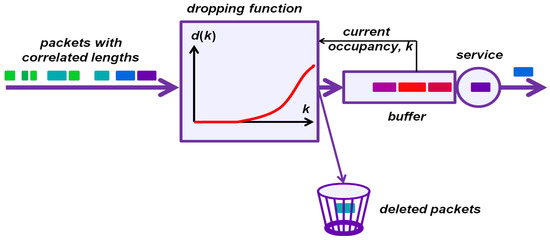
Figure 1.
Buffer with the dropping function and correlated packet lengths.
For this buffer model, four new mathematical results are obtained: a theorem on the buffer occupancy distribution at an arbitrary time t, a theorem on the buffer occupancy distribution in the steady state, a theorem on the average buffer occupancy at an arbitrary time t, and a theorem on the average buffer occupancy in the steady state.
Moreover, we present a comprehensive set of numerical results, showing the progression of the buffer occupancy distribution and the average value over time, its distribution and average value in the steady state, the impact on buffer occupancy of various dropping functions, correlation strengths, interarrival distributions, and buffer lengths. We also discuss the delay–loss tradeoff associated with the parameterization of the dropping function and validate the mathematical results via discrete-event computer simulations.
In the analysis, general interarrival distribution is assumed, enabling the modeling of any variance and higher moments of interarrival time. Moreover, the function is also assumed to have a general form, making the derived formulae applicable to any particular dropping function considered in the literature (a comprehensive list is supplied in the next section).
From a theoretical perspective, the model with dropping function generalizes the tail-drop model. Namely, by assuming if and if , we recover the tail-drop model with a buffer of length B packets. Thus, the results proven here incorporate previous findings on buffer occupancy under the tail-drop model with correlated packet lengths, but are much more general, as the dropping function may take an arbitrary shape here.
In a router, correlated packet lengths transmitted over an output link cause equivalent correlation in transmission times. Hence, correlated transmission times are equivalent to correlated packet lengths. Herein, we adopt the former approach. Namely, transmission times are modeled via the Markovian service process, known to allow simultaneous control of both the autocorrelation function of successive transmission times and the marginal distribution of transmission time. This makes it an ideal candidate for our study.
Detailed contributions of this article are as follows:
- Model of buffer with the dropping function and correlation of packet lengths;
- Theorem on buffer occupancy distribution at t (Theorem 1);
- Theorem on buffer occupancy distribution in steady state (Corollary 1);
- Theorem on average buffer occupancy at t (Theorem 2);
- Theorem on average buffer occupancy in steady state (Corollary 2);
- Numeric results showing the evolution of buffer occupancy (distribution and average value) in time, and in the steady state, for various dropping functions, correlation strengths, interarrival distributions and buffers lengths;
- Simulation results validating the mathematical formulae.
The rest of the document is formatted in the following manner. In Section 2, we first review prior research on active buffer management, including approaches founded on the dropping function and other methods. We then summarize the publications on buffers with correlated transmission times, modeled using the Markovian service process.
In Section 3, we present a formal model of the buffer incorporating both the dropping function and correlated transmission times. Section 4, which contains proofs of all four theorems concerning the buffer occupancy distribution and its average value, constitutes the core part of the work.
In Section 5, divided into Section 5.1, Section 5.2, Section 5.3, Section 5.4, Section 5.5, Section 5.6 and Section 5.7, we present numerical results. Specifically, in Section 5.1 we show the time evolution of the average buffer occupancy, the standard deviation, and the full distribution, for six distinct dropping functions. We also present the steady-state occupancy, the empty-buffer probability and the full-buffer probability.
In Section 5.2, the impact of correlation strength on buffer occupancy is demonstrated. We first compare results for correlated packet lengths with those for uncorrelated lengths to isolate the role of correlation in buffer occupancy. Then, we present and discuss the time-dependent and steady-state distributions of buffer occupancy for various correlation strengths.
Section 5.3 is devoted to the impact of the interarrival distribution on buffer occupancy, with an emphasis on its variance. Three interarrival distributions with different variances are used to compare the time-dependent evolution of buffer occupancy.
In Section 5.4, the combined influence of buffer length and the dropping function on buffer occupancy is illustrated. In Section 5.5, the practical delay–loss tradeoff associated with the parameterization of the dropping function is discussed and illustrated with two sample numerical solutions. Section 5.6 is devoted to verification, via simulation, of the theoretical steady-state formulae. Similarly, Section 5.7 demonstrates verification, via simulation, of the theoretical time-dependent formulae.
2. Related Work
As far as known by the authors, the results reported here are new. No previously published work has proposed or solved mathematically a buffer model with a dropping function and correlated packet lengths.
In general, active buffer management employs a variety of techniques beyond the dropping function (see, e.g., [3,4,5]). Some approaches are founded on control theory [6,7,8,9], others on neural networks [10,11,12,13], or fuzzy logic [14,15,16]. Certain methods determine the dropping probability exploiting packet sojourn time, rather than buffer occupancy (e.g., [17]).
Active management founded on the dropping function constitutes an appealing alternative because it offers relatively good performance while remaining very simple. It also represents a natural progression of the tail-drop policy, which is still commonly used.
As a result, the dropping function of numerous particular shapes has been studied in the literature, including linear [1], various polynomial forms [18,19,20], exponential [21], trigonometric [22], beta [23], Gaussian [24], and functions composed of several elementary components [25,26,27,28].
While most of the works [1,18,19,20,21,22,23,24,25,26,27,28] rely on simulations as the primary tool for performance evaluation, there are also several studies in which models founded on the dropping function are analyzed mathematically—mainly using methods from queueing theory (e.g., [29,30,31,32,33,34]). However, none of the models considered and solved in these works incorporated correlated packet lengths, which—as we will see here—considerably alter the performance of the dropping function.
Conversely, queueing models incorporating correlated packet lengths (via correlated service times) have been extensively studied in the literature, but never in combination with the dropping function mechanism (see, e.g., [35,36,37,38,39,40,41,42,43,44,45]).
The method used in this paper is based primarily on queueing theory. Specifically, a system of convolution integral equations for buffer occupancy is first constructed in the time domain. It is then solved in the Laplace transform domain. For other queueing-related problems solved using similar techniques, see, for example, [46,47].
This study is devoted to the mathematical model of a buffer with a dropping function and its solution via queueing theory. Practical aspects of applying the dropping function in networking are studied in [2]. Specifically, a prototype of a high-speed networking device implementing the dropping function mechanism in its buffer is described in detail, along with the results of experiments carried out with this device in an academic network.
3. Buffer Model
We focus on a packet buffer, in which packets are queued in the sequence they arrive. The buffer is emptied in the FIFO manner, starting from the front. The buffer can hold up to B packets, which number includes the packet in the process of transmission, if applicable. When there are B packets in the buffer, new arrivals are discarded.
This, however, is not the unique circumstance under which a packet can be discarded. Specifically, despite the buffer having free space, each arriving packet is subject to dropping. This takes place at random and has probability , where k denotes the buffer occupancy upon the packet arrival. Dropping function is not further specified here. For instance, it may take any form studied in [1,18,19,20,21,22,23,24,25,26,27,28].
The process of packet arrival is modeled by a general renewal process, parameterized by the interarrival distribution function . This distribution is also not specified, so that any particular G can be used.
In networking, the bandwidth of the link is usually constant, which results in packet transmission times being proportional to packet lengths. Therefore, correlation of packets lengths in the arrival process results in exactly the same correlation of transmission times, which will be modeled here via the Markovian service process [35].
The Markovian service process is parameterized by matrices, , of size , fulfilling the following three requirements: has non-negative elements except for the diagonal, where all entries are negative, has non-negative entries; is a transition-rate matrix, i.e., every row has the sum of 0. In other words, L is a transition-rate matrix for a Markov chain modulating the transmission process, with modulating states . Modulating state at time t will be denoted by .
In detail, the modulated transmission process evolves as follows. If and the buffer occupancy is nonzero at t, then at the modulating state may transition to j with probability , and the ongoing transmission of packet continues, or it may transition to j with probability , and the ongoing packet transmission is completed. When the transmission is not proceeding, due to lack of packets, the modulating state is not changing as well.
Summarizing, the full parameterization of the model consist of the buffer length B, dropping function , interarrival distribution , and matrices , .
The packet transmission rate is
where dentes the steady-state distribution for transition-rate matrix L, while
The load equals
where h symbolizes the average interarrival time
will stand for the buffer occupancy at t. includes in the process of transmission, if applicable at t.
The following notation style is used in the paper. Italic non-bold letters denote scalars, e.g., h, , , , B. Lowercase bold letters denote column vectors, e.g., , , . Uppercase bold letters denote square matrices, e.g., I, , . Furthermore, denotes probability, while denotes the expected value.
In Table 1, a compilation of the key notations used throughout the article is presented.

Table 1.
Key notations.
Finally, two characteristics of the Markovian service process will be of use: and . Firstly, is the probability that k transmissions are completed in interval , whereas the modulating state becomes j at time t, assuming and . Secondly, is the probability that k transmissions are completed in interval whereas the modulating state becomes j at the completion of the k-th transmission, assuming and .
4. Analysis
Our primary goal is to find
i.e., the probability of the buffer being occupied by k packets at time t, given the initial system conditions were , .
If initially the buffer is neither full nor empty, i.e, , then we have:
where the indicator is defined as:
The system of Equation (6) is secured by conditioning on the first arrival epoch, x. Four initial parts of (6) correspond to the event where . Specifically, the first part of (6) corresponds to the event, where in , m transmissions are completed and the modulating state changes to j, whereas the first incoming packet is discarded (probability ). Accordingly, the buffer occupancy at x remains whereas the modulating state becomes j. The second part of (6) corresponds to the event, where in , m transmissions are completed and the modulating state changes to j, but the first packet enters the buffer (probability ). Accordingly, the buffer occupancy at x becomes . Note also that in the first and the second part, it is presumed , thus the buffer occupancy cannot decrease to zero by x. The third part of (6) corresponds to the occurrence in which all n packets are sent from the buffer in period , the modulating state changes to j, and the first incoming packet is discarded (probability ). Therefore, the buffer contains no packets at x. The fourth part of (6) corresponds to the occurrence in which all n packets are transmitted from the buffer in period , the modulating state changes to j, but the first packet enters the buffer (probability ). The buffer occupancy at x becomes 1. The last, fifth part of (6) corresponds to the event where the first packet arrives after t (probability ). Under such event, we can just calculate the probability of a non-empty () and empty () buffer at t, using function .
If the buffer is completely filled at , we obtain
Equation (8) is procured likewise (6), with the exception of the second parts of (6) and (8), which differ from each other. Specifically, if , then it is impossible to have no transmissions completed in , and to allow a new packet to the buffer at x, because the buffer would still be full at such a case. Therefore, the summation over m in the second term of (8) must begin with , rather than with , as in the case of system (6).
If the buffer contains no packets at , we obtain
Equation (9) is secured again by conditioning on the first arrival epoch, x. No transmissions can be completed from an empty buffer, thus functions and are not involved. The three parts of (9) simply cover the three events: the first packet arrives prior to t and is discarded, the first packet arrives prior to t and enters the buffer, the first packet arrives after t. In the latter event, the buffer remains empty at t, so only is possible.
As we see, (6), (8), and (9) constitute a system of convolution integral equations. We shall resolve this system now making use of the Laplace transform and matrix notation.
Denote:
Observing that:
and applying Convolution Theorem (see, e.g., Theorem 2.39 of [48]) to (6), (8), and (9), we obtain
and
respectively. Then, denoting
from (16) we have
with
As we see, system (23), (25), and (26) is linear and can now be easily solved with help of linear algebra. The solution can be expressed using a vector of length :
and presented as the following theorem.
Theorem 1.
To make Theorem 1 fully functional in numeric calculations, we need a few additional components. First, we must be able to calculate matrices , and , visible in (31), and (24). To calculate and , we may apply directly the uniformization technique (see [49]). Applying this technique, we have
where
and
Having and , we can calculate using formulae (55)–(57) of [44], namely:
where
Now all the components of Theorem 1 are known. However, (29) is expressed in the Laplace transform domain. Therefore, the last step needed to obtain is inversion of (29) to time domain. We exploit the Zakian’s formula [50], in the numeric examples of Section 5.
Now, we can also establish the steady-state occupancy distribution.
Note first that the system defined in Section 3 is always stable, regardless of the value of . This follows from the finite-buffer assumption, i.e., the fact that the buffer occupancy cannot exceed B. The proof is exactly the same as in the case of the classic M/G/1/B queueing model; see Section 3 of the monograph [51].
For a stable system, we can define
From Theorem 1 and Theorem 2.36 of [48], we obtain as follows.
Corollary 1.
In numeric examples, it usually suffices to use s about in (45), at which value of s a rather good convergence to is achieved.
Our next goal is to derive
i.e., the average buffer occupancy at t, given the initial system conditions were , . Naturally, this can be achieved using the relation
and Theorem 1. This strategy, however, requires separate calculations of every and application of the transform inversion formula times. Therefore, below we propose an alternative approach, which will require only one application of the inversion formula.
Specifically, we can procure equations analogous to (6), (8), and (9), but for rather than . Specifically, for we have
which is secured through the same process as (6). For we obtain analogously:
while for :
System (48), (49), (50) differs from system (6), (8), (9) only with regards to constant elements. Accordingly, it can be solved in the same fashion, which gives the following outcome.
Theorem 2.
Average buffer occupancy at t has transform:
where
Now, defining
from Theorem 2 and Theorem 2.36 of [48], we obtain the final theoretical result.
5. Numeric Examples
5.1. Dependence on the Dropping Function
To check the dependence of the buffer occupancy on the dropping function form, in this subsection we use many different dropping functions belonging to the following class:
where a denotes a positive parameter. For , this class is depicted in Figure 2.
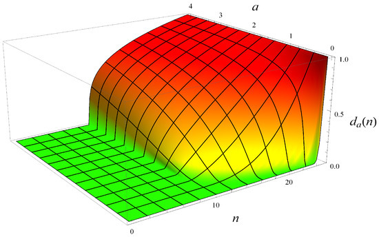
Figure 2.
Class of dropping functions (57) vs. parameter a.
As we see, the larger a, the stronger the dropping function, i.e., the larger the dropping probabilities. For , the dropping function is convex on its operational range, ; for , it is linear; while for , it becomes concave. Moreover, as , the buffer policy approaches the tail-drop policy with a buffer length of packets. Therefore, the case will also be referred to as the “no dropping function” case.
Packet transmission times are parameterized by matrices as follows:
These matrices were generated randomly to yield a moderate correlation coefficient of 0.3 between two consecutive transmission times, an average transmission time of 1.0, and a standard deviation of 1.0. The latter fact allows us to isolate the pure effect of correlation—separated from the influence of standard deviation—when comparing the results with the case of exponential i.i.d. transmission times.
Finally, the following hyperexponential distribution is exploited for the time between successive packets:
which gives the arrival rate:
Therefore, the load is . Moreover, the standard deviation for equals 1.64, which makes the arrival traffic significantly non-Poisson.
In Figure 3 and Figure 4, the time evolution of the average buffer occupancy and standard deviation are presented, respectively. Each figure includes six different dropping functions, ranging from a very mild one () to a very strong one ().
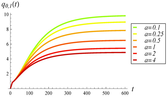
Figure 3.
Average buffer occupancy vs. time for various dropping functions.
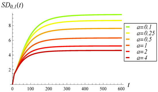
Figure 4.
Standard deviation of buffer occupancy vs. time for various dropping functions.
As shown in Figure 3 and Figure 4, increasing a (i.e., applying stronger dropping) has three main effects. First, the average buffer occupancy decreases significantly with increasing a, which is an expected outcome. Second, the standard deviation also decreases with a in a similar fashion. Third, the duration until convergence to steady state becomes slightly shorter as a increases. For mild dropping (), the average buffer occupancy approaches the steady state limit in approximately 600 time units. For strong dropping (), this is reduced to around 400 time units. Note that both convergence times—400 and 600—can be considered long. As we will see later, this prolonged convergence is caused by the correlation in transmission times.
In Figure 5 and Figure 6, the time evolution of the full-buffer probability and the empty-buffer probability is presented, respectively. As before, each figure includes six different dropping functions, ranging from to .
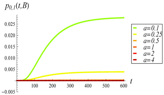
Figure 5.
Full-buffer probability vs. time for various dropping functions.
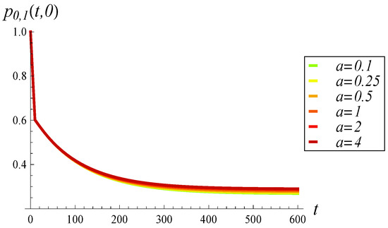
Figure 6.
Empty-buffer probability vs. time for various dropping functions.
A stark contrast can be observed between Figure 5 and Figure 6. Specifically, increasing a exerts a considerable effect on the full-buffer probability, significantly reducing it, while it has virtually no effect on the empty-buffer probability.
In Figure 7, the steady-state average occupancy and standard deviation are shown as functions of a. We observe that, by adjusting a, the average buffer occupancy can be controlled to a significant extent. Specifically, for , the average occupancy is , while for , it drops to . Hence, any average occupancy within the interval can be achieved by choosing an appropriate value of a.
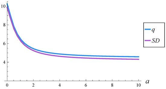
Figure 7.
Steady-state average buffer occupancy, q, and the standard deviation, , vs. parameter a of the dropping function.
As shown in Figure 7, the standard deviation exhibits a very similar dependence on a as the average occupancy.
In Figure 8, Figure 9 and Figure 10, the time evolution of the complete buffer occupancy distribution is depicted. Specifically, Figure 8 shows the distribution when no dropping function is applied; Figure 9 corresponds to a mild dropping function (); and Figure 10 illustrates the case of a strong dropping function ().
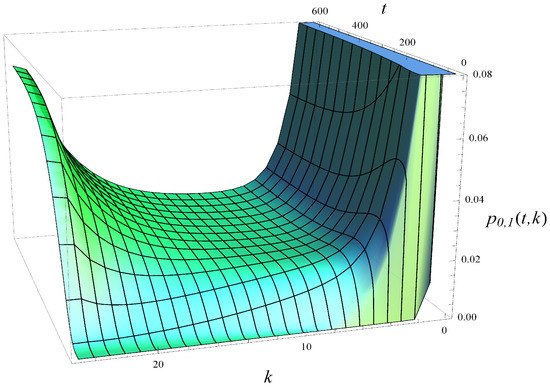
Figure 8.
Distribution of buffer occupancy vs. time. No dropping function, .
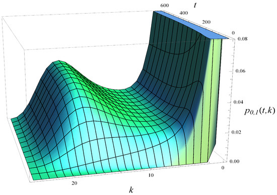
Figure 9.
Distribution of buffer occupancy vs. time. Mild dropping function, .
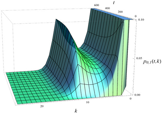
Figure 10.
Distribution of buffer occupancy vs. time. Strong dropping function, .
As we observe, without the dropping function (Figure 8), the probability mass becomes concentrated around and over time. The application of a mild dropping function (Figure 9) shifts the concentration to around and . When a strong dropping function is applied (Figure 10), the probability mass concentrates near and , effectively eliminating buffer occupancies greater than 16.
In the next section, we will check the impact of correlation on the buffer occupancy distribution.
5.2. Dependence on the Correlation
So far, we have analyzed the behavior of the buffer occupancy determined by the dropping function strength.
Now, let us examine to what extent the observed behavior may be credited to the correlated transmission times. To do this, we compare first the buffer performance with transmissions governed by matrices (58) and (59) against a buffer with i.i.d. exponential transmission times, both having the same average transmission time and standard deviation equal to 1. Thus, the average transmission time and standard deviation are identical in both cases. The distinction is that, in scenarios with matrices (58) and (59), there is an additional correlation of 0.3 between two consecutive transmission times.
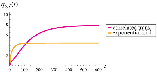
The results of this comparison are shown in Figure 11, Figure 12 and Figure 13. Specifically, Figure 11 presents the average occupancy without applying the dropping function; Figure 12 corresponds to a mild dropping function (); and Figure 13 illustrates the case of a strong dropping function ().
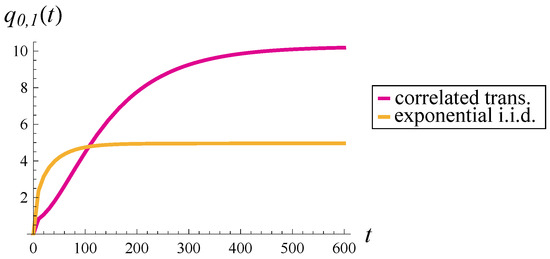
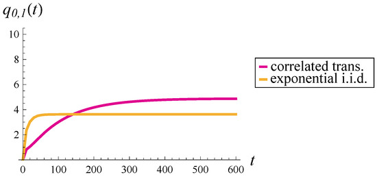
As seen in Figure 11, correlation has a significant impact on two aspects of buffer performance. First, reaching the steady-state limit takes about six times longer in the correlated case (approximately 600 vs. 100 time units). Second, the steady-state occupancy is more than twice as large when transmissions are correlated.
With a mild dropping function applied (Figure 12), the steady-state occupancy is reduced by about 25% in the correlated case, but shows very little change in the uncorrelated case. Convergence times remain practically unchanged.
When a strong dropping function is applied (Figure 13), the steady-state occupancy decreases by as much as 50% in the correlated case. Roughly speaking, the correlated case with a strong dropping function becomes closer to the uncorrelated case without any dropping function (compare the orange line in Figure 11 with the purple line in Figure 13). The line for uncorrelated transmissions in Figure 13 is also affected by the dropping function, but to a much lesser extent than the correlated one. Convergence times are shortened in both cases, though the convergence time in the correlated case remains several times larger than in the uncorrelated case.
We may also compare the impact of correlation with various strengths on buffer occupancy. To accomplish this, two additional parameterizations of the service will be used. Specifically, to achieve a correlation coefficient of 0.2 between two consecutive service times, we set:
where , are given in (58) and (59), respectively. To achieve the correlation coefficient of 0.1 between two consecutive service times, we set:
The original parameters (58) and (59) produce a correlation of 0.3, while zero correlation can be achieved, as before, using exponential i.i.d. service times with . Importantly, all four parameterizations yield the same service rate of 1.
In Figure 14, the steady-state average occupancy is shown as a function of the parameter a of the dropping function (57).
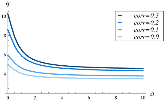
Figure 14.
Steady-state average buffer occupancy, q, vs. parameter a, for four service parameterizations of various correlation strengths.
We observe that the correlation strength has a strong influence on occupancy for every value of a. The stronger the correlation, the greater the average buffer occupancy. This influence is more pronounced when the dropping function is mild (i.e., a is small). In such cases, the occupancy can be twice as high for a correlation of 0.3 compared to a correlation of 0. When the dropping function is aggressive (large a), the occupancy is about 1.2 times higher for a correlation of 0.3 than for a correlation of 0.
In Figure 15, Figure 16 and Figure 17, the buffer occupancy distribution at distinct moments in time is presented. The three figures differ in the strength of the correlation used. Specifically, Figure 15 was obtained for a correlation of 0.1, Figure 16 for a correlation of 0.2, and Figure 17 for a correlation of 0.3.
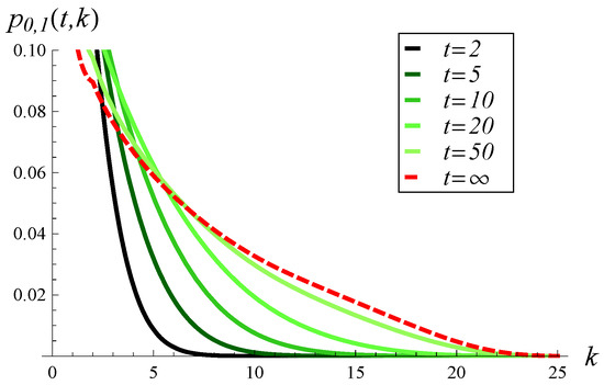
Figure 15.
Buffer occupancy distribution at different moments in time, for the correlation of 0.1 and .
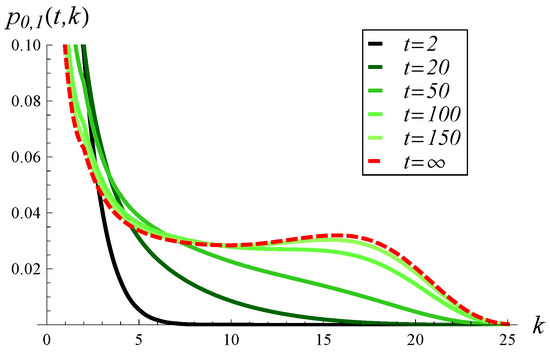
Figure 16.
Buffer occupancy distribution at different moments in time, for the correlation of 0.2 and .
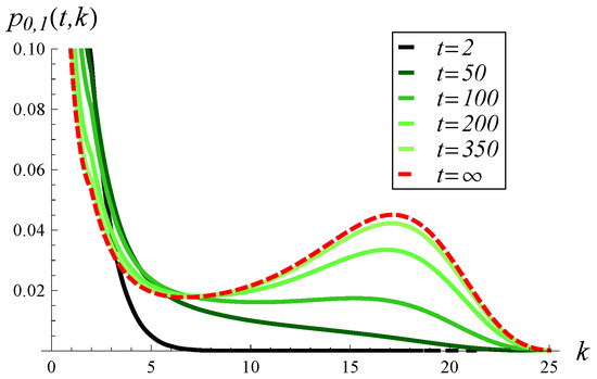
Figure 17.
Buffer occupancy distribution at different moments in time, for the correlation of 0.3 and .
As we see, the correlation strength affects the time-dependent buffer occupancy in at least two ways. First, the convergence time to the steady state increases as the correlation becomes stronger. Specifically, in Figure 15, the distribution of occupancy becomes close to the steady-state distribution at . In Figure 16, the distribution approaches the steady state at , while in Figure 17 it does so at .
Second, the shape of the distribution is affected by the correlation strength. For weak correlation, the distribution has a single mode at for every t considered (see Figure 15). When the correlation becomes stronger, a more complex, two-mode distribution occurs, with modes at and (see Figure 16 and Figure 17).
In the next section, we will examine how the variance of the interarrival time distribution influences buffer occupancy.
5.3. Dependence on the Interarrival Time
So far, we have used only one interarrival distribution, (60), with the average value of 1.25 and the standard deviation of 1.64. In this subsection, we will use two more interarrival distributions, namely:
with the average of 1.25 and the standard deviation of 3.0, and
with the average of 1.25 and the standard deviation of 5.0. Therefore, we now have three interarrival distributions available, , , and , with a common average of 1.25 but standard deviations of 1.64, 3.0, and 5.0, respectively. In addition, the service matrices (58) and (59) will be used, along with the dropping function (57) with .
In Figure 18, the average buffer occupancy over time is presented for the three interarrival distributions. In the steady-state limit, a greater standard deviation corresponds to a lower occupancy, although the differences are not large. This can perhaps be explained by the fact that greater variability in the arrival process induces more packet losses, which decreases the effective load carried by the buffer.
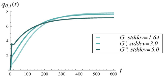
Figure 18.
Average buffer occupancy vs. time for interarrival distributions of different standard deviations.
In the transient regime, up to about , the reverse effect can be observed, i.e., a greater standard deviation corresponds to a higher occupancy. Moreover, a sharp peak is visible in the curve. To examine this more closely, a short period up to is enlarged in Figure 19.
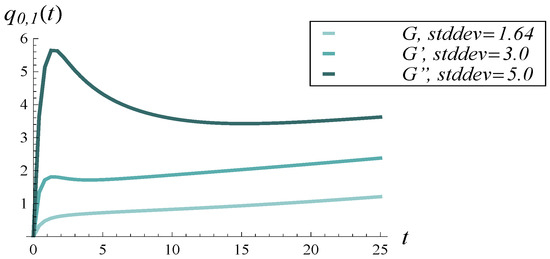
Figure 19.
Average buffer occupancy vs. time for interarrival distributions of different standard deviations. Short time period.
As seen in Figure 19, when the standard deviation of the interarrival time is large, the evolution of the average buffer occupancy can be non-monotone in the short initial period, with possible local maxima and minima.
In the next section, we will see how the buffer length, together with the dropping function, may affect buffer occupancy.
5.4. Dependence on the Buffer Length
Previously, the buffer length was constant and equal to packets. In this subsection, we vary the buffer length from up to packets. The dropping function is now linear (RED-type) and always operates on the second half of the buffer, regardless of its length. Specifically, the following dropping function is used:
where B is a parameter (buffer length), which will be changed from 2 to 1000. (Note that changing B, which simultaneously change the buffer length and the dropping function.) Furthermore, the interarrival distribution (60) and service matrices (58) and (59) are used.
Under these settings, the resulting average buffer occupancy as a function of the buffer length is depicted in Figure 20. As we see, the average occupancy grows with B, but not indefinitely. At B about 800 packets, it stops growing. At this point, the dropping function ceases to operate, i.e., the buffer occupancy rarely enters the operation range of the dropping function, .
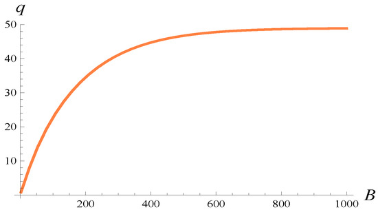
Figure 20.
Average buffer occupancy in the steady state versus buffer length in (66).
Note, however, that this behavior can be attributed to the load, which is less than 1 (we have ). For , the average buffer occupancy would grow with B indefinitely.
In the next section, we will discuss the delay–loss tradeoff associated with the parameterization of the dropping function.
5.5. Delay–Loss Tradeoff
By manipulating the dropping function and the buffer length, we can adjust the average buffer occupancy to our needs. For instance, varying B from 2 to 1000 in (66), we can obtain any value of the average occupancy in the range (see Figure 20). However, applying a more aggressive dropping function (small B in (66)) reduces the buffer occupancy at the cost of increasing the packet loss probability, .
A desired tradeoff between the two characteristics can be achieved by computing the empty-buffer probability, , using Corollary 1, and then exploiting the well-known relation between and . Namely, we have
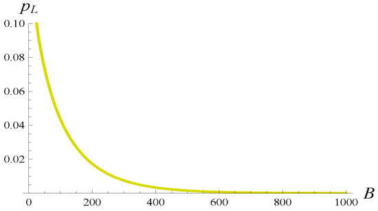
Figure 21.
Loss probability versus buffer length in (66).
Now, by combining Figure 20 with Figure 21, we can navigate the delay–loss tradeoff according to our requirements. For instance, we may ask which parameterization of (66) provides a minimal buffering delay with the loss probability less than 0.01. From Figure 21, it follows that setting yields . For , we also have (see Figure 20), which is the minimal average occupancy achievable with .
Alternatively, we may ask which parameterization of (66) provides a minimal loss probability while maintaining the average occupancy below 20 packets. From Figure 20, it follows that setting yields . For , we also have (see Figure 21), which is the minimal loss probability if we insist on .
Finally, note that the presented tradeoffs were obtained for the class of dropping functions (66). For other parameter-dependent classes, these tradeoffs may differ.
The following two sections are devoted to the verification of the theoretical formulas by means of computer simulations.
5.6. Verification via Simulations: Steady State
We also verified the correctness of the theoretical results through simulations. Specifically, the model of Section 3 was implemented in the OMNeT++ simulator [52].
To simulate steady-state results, in each simulation run packets crossing the buffer were simulated. During each run, the buffer occupancy was recorded at regular intervals of 1 time unit, thereby building a histogram. Finally, the histogram’s average value and standard deviation were calculated. Ten simulation runs were executed, each corresponding to a distinct parameterization of the dropping function according to (57). Service parameters (58) and (59) were used.
The results are displayed in Table 2, where the simulation outputs are compared to the theoretical results. We observe excellent agreement between the simulated and theoretical steady-state results in every considered scenario—the maximal relative error is 0.2%.
Table 2.
Theoretical and simulated values of the average buffer occupancy and standard deviation for various dropping functions (steady state).
5.7. Verification via Simulations: Time-Dependent Case
To obtain time-dependent characteristics via simulations, a different approach was used. Roughly speaking, instead of a few rather long simulation runs, as in the previous section, a large number of short runs were executed.
Specifically, to obtain the buffer occupancy distribution at a particular t, say , 50,000 identical simulation runs were performed. Each simulation run began with an empty buffer and modulating state 1 and lasted until the simulated time reached the predefined . The only difference between these runs was the RNG seed. At the end of each run, the buffer occupancy was recorded and placed into a histogram. Finally, after 50,000 runs, the histogram’s average value and standard deviation were calculated.
This procedure was repeated for ten different settings of time t, varying from up to . Therefore, separate simulation runs were carried out in total. Service parameters (58) and (59), and in (57) were used.
The results are displayed in Table 3, where the simulation outputs are compared to their theoretical counterparts. We again observe excellent agreement between the simulated and theoretical results for every considered moment in time. The maximal relative error is 0.8%, and in most cases it is far less than that.
Table 3.
Theoretical and simulated values of the average buffer occupancy and standard deviation at various moments in time.
6. Study Limitations
The model studied here has several limitations.
First, the length of the buffer is finite. From an application perspective, this is not a drawback—all real electronic devices have buffers of finite lengths, bounded by memory. Moreover, as argued in Section 4, the evolution of buffer occupancy is stable regardless of the value of when the buffer is finite. On the other hand, a model with an infinite buffer would provide a theoretical insight into the limiting behavior of the system, when the queue is not artificially limited by a cap on the maximum queue length. Furthermore, a model with an infinite buffer may perhaps allow a more compact formulation of the main characteristics, as is the case with classic models. For instance, the formulas for performance characteristics of the M/G/1 model are more compact than those for the M/G/1/N model.
A model with an infinite buffer and a dropping function would first require finding and proving the stability condition, involving both and . The classic stability condition for systems without a dropping function, i.e., , cannot be transferred to a system with a dropping function. It is easy to see that a system with a dropping function can be stable even if , provided an aggressive dropping function is applied. For instance, if but for every k, then the system is stable.
The second limitation of the model is that interarrival times are assumed to be mutually independent. In reality, interarrival times can be correlated and bursty to varying degrees. Such phenomena cannot be captured using the model of Section 3, and the formulas proven here may produce large errors when applied to strongly correlated traffic. To overcome this, one of the available models of correlated interarrival times can be used, in addition to the Markovian service process used on the service side.
Third, the service time distribution (MSP) is Markovian here. Models with other, non-Markovian correlated service times can be studied as well.
7. Conclusions
We analyzed the buffer occupancy in a new packet buffer model where a packet can be discarded with a probability connected to the buffer occupancy through an arbitrary dropping function. Crucially, it was assumed that packet lengths can be correlated in any manner and that interarrival times follow a general distribution. The considered model generalizes many specific active buffer management algorithms proposed for Internet routers, which use particular elementary functions or their combinations as dropping functions. It also extends the class of finite-buffer models with the tail-drop discarding policy.
The contributions include four new theorems concerning the buffer occupancy distribution and the average occupancy, at arbitrary time t and also in the steady state. These theorems were illustrated through numerical calculations of the average buffer occupancy, its standard deviation, full-buffer probability, empty-buffer probability, and the complete distribution of buffer occupancy in the steady-state and also in time-dependent cases. The calculations were performed for various dropping functions with differing levels of aggressiveness, for various correlation strengths, various interarrival distributions, and buffer lengths. From a practical perspective, we discussed the delay–loss tradeoff associated with the parameterization of the dropping function and buffer length. We also validated the mathematical results via discrete-event computer simulations.
This study has two main practical implications:
- Knowing the dropping function and the traffic, we can compute the average buffer occupancy and, consequently, the average delay added by the buffering mechanism to the transmission path of a packet.
- Alternatively, we can parameterize the dropping function so that it provides a particular value for the average buffer occupancy (delay) or satisfies a delay–loss tradeoff.
Several possible directions for future research arise from the limitations discussed in the previous section.
First, a model with correlated service, a dropping function, and an infinite buffer can be analyzed. Specifically, a general stability condition involving and should be established first, followed by a study of detailed performance characteristics.
Second, a model with correlated service, a dropping function, and correlated interarrival times can be investigated, using one of the available models for correlated interarrival times, e.g., the Markov-modulated Poisson process (MMPP), the Markovian arrival process (MAP), or the batch Markovian arrival process (BMAP).
Another direction for future research is to further study the same model as here, but with respect to additional performance characteristics, including the waiting time distribution, busy period distribution, or characterization of the output traffic.
Author Contributions
Conceptualization, A.C.; methodology, A.C.; software, A.C.; validation, A.C. and B.A.; formal analysis, A.C. and B.A.; investigation, A.C. and B.A.; writing—original draft preparation, A.C.; writing—review and editing, A.C. and B.A.; visualization, A.C.; supervision, A.C. All authors have read and agreed to the published version of the manuscript.
Funding
This research received no external funding.
Data Availability Statement
Data is contained within the article.
Conflicts of Interest
The authors declare no conflicts of interest.
References
- Floyd, S.; Jacobson, V. Random early detection gateways for congestion avoidance. IEEE/Acm Trans. Netw. 1993, 1, 397–413. [Google Scholar] [CrossRef]
- Barczyk, M.; Chydzinski, A. AQM based on the queue length: A real-network study. PLoS ONE 2022, 17, e0263407. [Google Scholar] [CrossRef]
- de Morais, W.G.; Santos, C.E.M.; Pedroso, C.M. Application of active queue management for real-time adaptive video streaming. Telecommun. Syst. 2022, 79, 261–270. [Google Scholar] [CrossRef]
- Li, Z.; Hu, Y.; Tian, L.; Lv, Z. Packet rank-aware active queue management for programmable flow scheduling. Comput. Netw. 2023, 225, 109632. [Google Scholar] [CrossRef]
- Lhamo, O.; Lhamo, O.; Ma, M.; Doan, T.V.; Scheinert, T.; Nguyen, G.T.; Reisslein, M.; Fitzek, F.H. RED-SP-CoDel: Random early detection with static priority scheduling and controlled delay AQM in programmable data planes. Comput. Commun. 2024, 214, 149–166. [Google Scholar] [CrossRef]
- Kahe, G.; Jahangir, A.H. A self-tuning controller for queuing delay regulation in TCP/AQM networks. Telecommun. Syst. 2019, 71, 215–229. [Google Scholar] [CrossRef]
- Belamfedel Alaoui, S.; Tissir, E.H.; Chaibi, N. Analysis and design of robust guaranteed cost Active Queue Management. Comput. Commun. 2020, 159, 124–1321. [Google Scholar] [CrossRef]
- Wang, H. Trade-off queuing delay and link utilization for solving bufferbloat. ICT Express 2020, 6, 269–272. [Google Scholar] [CrossRef]
- Hotchi, R.; Chibana, H.; Iwai, T.; Kubo, R. Active queue management supporting TCP flows using disturbance observer and Smith predictor. IEEE Access 2020, 8, 173401–173413. [Google Scholar] [CrossRef]
- Li, F.; Sun, J.; Zukerman, M.; Liu, Z.; Xu, Q.; Chan, S.; Chen, G.; Ko, K.T. A comparative simulation study of TCP/AQM systems for evaluating the potential of neuron-based AQM schemes. J. Netw. Comput. Appl. 2014, 41, 274–299. [Google Scholar] [CrossRef]
- Chrost, L.; Chydzinski, A. On the deterministic approach to active queue management. Telecommun. Syst. 2016, 63, 27–44. [Google Scholar] [CrossRef]
- Wang, C.; Chen, X.; Cao, J.; Qiu, J.; Liu, Y.; Luo, Y. Neural Network-Based Distributed Adaptive Pre-Assigned Finite-Time Consensus of Multiple TCP/AQM Networks. IEEE Trans. Circuits Syst. 2021, 68, 387–395. [Google Scholar] [CrossRef]
- Song, T.; Kyung, Y. Deep-Reinforcement-Learning-Based Age-of-Information-Aware Low-Power Active Queue Management for IoT Sensor Networks. IEEE Internet Things J. 2024, 11, 16700–16709. [Google Scholar] [CrossRef]
- Chen, W.; Wang, W.; Jiang, Y.; Li, G.; Chen, Q. PFL: Proactive Fuzzy-logic-based AQM Algorithm for Best-effort Networks. In Proceedings of the 2010 International Conference on Computational Aspects of Social Networks, Taiyuan, China, 26–28 September 2010; pp. 315–318. [Google Scholar]
- Chen, J.V.; Chen, F.C.; Tarn, J.M.; Yen, D.C. Improving network congestion: A RED-based fuzzy PID approach. Comput. Stand. Interfaces 2012, 34, 426–438. [Google Scholar] [CrossRef]
- Shen, J.; Jing, Y.; Ren, T. Adaptive finite time congestion tracking control for TCP/AQM system with input saturation. Int. J. Syst. Sci. 2022, 53, 253–264. [Google Scholar] [CrossRef]
- Nichols, K.; Jacobson, V. Controlling Queue Delay. Queue 2012, 55, 42–50. [Google Scholar]
- Zhou, K.; Yeung, K.L.; Li, V. Nonlinear RED: Asimple yet efficient active queue management scheme. Comput. Netw. 2006, 50, 3784. [Google Scholar] [CrossRef]
- Augustyn, D.R.; Domanski, A.; Domanska, J. A choice of optimal packet dropping function for active queue management. Commun. Comput. Inf. Sci. 2010, 79, 199–206. [Google Scholar] [CrossRef] [PubMed]
- Domanska, J.; Augustyn, D.; Domanski, A. The choice of optimal 3-rd order polynomial packet dropping function for NLRED in the presence of self-similar traffic. Bulletin of the Polish Academy of Sciences. Tech. Sci. 2012, 60, 779–786. [Google Scholar]
- Hussein, A.-J. An Exponential Active Queue Management Method Based on Random Early Detection. J. Comput. Netw. Commun. 2020, 2020, 8090468. [Google Scholar]
- Zhang, S.; Sa, J.; Liu, J.; Wu, S. An improved RED algorithm with sinusoidal packet-marking probability and dynamic weight. In Proceedings of the 2011 International Conference on Electric Information and Control Engineering, Wuhan, China, 15–17 April 2011; pp. 1160–1163. [Google Scholar]
- Gimenez, A.; Murcia, M.A.; Amigó, J.M.; Martínez-Bonastre, O.; Valero, J. New RED-Type TCP-AQM Algorithms Based on Beta Distribution Drop Functions. Appl. Sci. 2022, 12, 11176. [Google Scholar] [CrossRef]
- Mahajan, M.; Singh, T.P. The Modified Gaussian Function based RED (MGF-RED) Algorithm for Congestion Avoidance in Mobile Ad Hoc Networks. Int. J. Comput. Appl. 2014, 91, 39–44. [Google Scholar] [CrossRef]
- Feng, C.; Huang, L.; Xu, C.; Chang, Y. Congestion Control Scheme Performance Analysis Based on Nonlinear RED. IEEE Syst. J. 2017, 11, 2247–2254. [Google Scholar] [CrossRef]
- Patel, S.; Karmeshu. A New Modified Dropping Function for Congested AQM Networks. Wirel. Pers. Commun. 2019, 104, 37–55. [Google Scholar] [CrossRef]
- Hassan, S.O.; Nwaocha, V.O.; Rufai, A.U.; Odule, T.J.; Enem, T.A.; Ogundele, L.A.; Usman, S.A. Random early detection-quadratic linear: An enhanced active queue management algorithm. Bull. Electr. Eng. Inform. 2022, 11, 2262–2272. [Google Scholar] [CrossRef]
- Hassan, S.O.; Rufai, A. Modified dropping-random early detection (MD-RED): A modified algorithm for controlling network congestion. Int. J. Inf. Technol. 2023, 15, 1499–1508. [Google Scholar] [CrossRef]
- Bonald, T.; May, M.; Bolot, J.-C. Analytic evaluation of RED performance. In Proceedings of the Proceedings IEEE INFOCOM 2000. Conference on Computer Communications. Nineteenth Annual Joint Conference of the IEEE Computer and Communications Societies (Cat. No.00CH37064), Tel Aviv, Israel, 26–30 March 2000; pp. 1415–1424. [Google Scholar]
- Hao, W.; Wei, Y. An Extended GIX/M/1/N Queueing Model for Evaluating the Performance of AQM Algorithms with Aggregate Traffic. Lect. Notes Comput. Sci. 2005, 3619, 395–414. [Google Scholar]
- Kempa, W.M. Time-dependent queue-size distribution in the finite GI/M/1 model with AQM-type dropping. Acta Electrotech. Inform. 2013, 13, 85–90. [Google Scholar] [CrossRef]
- Tikhonenko, O.; Kempa, W.M. Performance evaluation of an M/G/N-type queue with bounded capacity and packet dropping. Appl. Math. Comput. Sci. 2016, 26, 841–854. [Google Scholar] [CrossRef]
- Tikhonenko, O.; Kempa, W.M. Erlang service system with limited memory space under control of AQM mechanizm. Commun. Comput. Inf. Sci. 2017, 718, 366–379. [Google Scholar]
- Chydzinski, A. Queues with the dropping function and non-Poisson arrivals. IEEE Access 2020, 8, 39819–39829. [Google Scholar] [CrossRef]
- Bocharov, P.P.; D’Apice, C.; Pechinkin, A.V.; Salerno, S. The stationary characteristics of the G/MSP/1/r queueing system. Autom. Remote Control 2003, 64, 288–301. [Google Scholar] [CrossRef]
- Gupta, U.C.; Banik, A.D. Complete analysis of finite and infinite buffer GI/MSP/1 queue—a computational approach. Oper. Res. Lett. 2007, 35, 273–280. [Google Scholar] [CrossRef]
- Banik, A.D. Analyzing state-dependent arrival in GI/BMSP/1/∞ queues. Math. Comput. Model. 2011, 53, 1229–1246. [Google Scholar] [CrossRef]
- Chaudhry, M.L.; Samanta, S.K.; Pacheco, A. Analytically explicit results for the GI/C-MSP/1/∞ queueing system using roots. Probab. Eng. Inform. Sci. 2012, 26, 221–244. [Google Scholar] [CrossRef]
- Samanta, S.K. Sojourn-time distribution of the GI/MSP/1 queueing system. Opsearch 2015, 52, 756–770. [Google Scholar] [CrossRef]
- Chaudhry, M.L.; Banik, A.D.; Pacheco, A. A simple analysis of the batch arrival queue with infinite-buffer and Markovian service process using roots method: GIX/C-MSP/1/∞. Ann. Oper. Res. 2017, 252, 135–173. [Google Scholar] [CrossRef]
- Banik, A.D.; Chaudhry, M.L.; Kim, J.J. A Note on the Waiting-Time Distribution in an Infinite-Buffer GI[X]/C-MSP/1 Queueing System. J. Probab. Stat. 2018, 2018, 7462439. [Google Scholar] [CrossRef]
- Banik, A.D.; Ghosh, S.; Chaudhry, M.L. On the consecutive customer loss probabilities in a finite-buffer renewal batch input queue with different batch acceptance/rejection strategies under non-renewal service. In Soft Computing for Problem Solving: SocProS 2017; Springer: Singapore, 2019; Volume 1, pp. 45–62. [Google Scholar]
- Banik, A.D.; Ghosh, S.; Chaudhry, M.L. On the optimal control of loss probability and profit in a GI/C-BMSP/1/N queueing system. Opsearch 2020, 57, 144–162. [Google Scholar] [CrossRef]
- Chydzinski, A. Transient GI/MSP/1/N Queue. Entropy 2024, 26, 807. [Google Scholar] [CrossRef]
- Samanta, S.K.; Bank, B. Modelling and Analysis of GI/BMSP/1 Queueing System. Bull. Malays. Math. Sci. Soc. 2021, 44, 3777–3807. [Google Scholar] [CrossRef]
- Chydzinski, A. Transient Analysis of the MMPP/G/1/K Queue. Telecommun. Syst. 2006, 32, 247–262. [Google Scholar] [CrossRef]
- Chydzinski, A.; Adamczyk, B. Transient and stationary losses in a finite-buffer queue with batch arrivals. Math. Probl. Eng. 2012, 2012, 326830. [Google Scholar] [CrossRef]
- Schiff, J.L. The Laplace Transform: Theory and Applications; Springer: New York, NY, USA, 1999. [Google Scholar]
- Dudin, A.N.; Klimenok, V.I.; Vishnevsky, V.M. The Theory of Queuing Systems with Correlated Flows; Springer: Cham, Swizterland, 2020. [Google Scholar]
- Zakian, V. Numerical inversion of Laplace transform. Electron. Lett. 1969, 5, 120–121. [Google Scholar] [CrossRef]
- Cohen, J.W. The Single Server Queue, Revised ed.; North-Holland Publishing Company: Amsterdam, The Netherlands, 1982. [Google Scholar]
- Available online: https://omnetpp.org/ (accessed on 1 August 2025).


Disclaimer/Publisher’s Note: The statements, opinions and data contained in all publications are solely those of the individual author(s) and contributor(s) and not of MDPI and/or the editor(s). MDPI and/or the editor(s) disclaim responsibility for any injury to people or property resulting from any ideas, methods, instructions or products referred to in the content. |
© 2025 by the authors. Published by MDPI on behalf of the International Institute of Knowledge Innovation and Invention. Licensee MDPI, Basel, Switzerland. This article is an open access article distributed under the terms and conditions of the Creative Commons Attribution (CC BY) license (https://creativecommons.org/licenses/by/4.0/).